CHAPTER

7

Signaling over AWGN Channels

7.1    Introduction

Chapter 6 on the conversion of analog waveforms into coded pulses represents the transition from analog communications to digital communications. This transition has been empowered by several factors:

1.  Ever-increasing advancement of digital silicon chips, digital signal processing, and computers, which, in turn, has prompted further enhancement in digital silicon chips, thereby repeating the cycle of improvement.

2.  Improved reliability, which is afforded by digital communications to a much greater extent than is possible with analog communications.

3.  Broadened range of multiplexing of users, which is enabled by the use of digital modulation techniques.

4.  Communication networks, for which, in one form or another, the use of digital communications is the preferred choice.

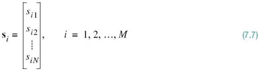
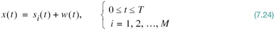
In light of these compelling factors, we may justifiably say that we live in a “digital communications world.” For an illustrative example, consider the remote connection of two digital computers, with one computer acting as the information source by calculating digital outputs based on observations and inputs fed into it; the other computer acts as the recipient of the information. The source output consists of a sequence of 1s and 0s, with each binary symbol being emitted every T_b seconds. The transmitting part of the digital communication system takes the 1s and 0s emitted by the source computer and encodes them into distinct signals denoted by s₁(t) and s₂(t), respectively, which are suitable for transmission over the analog channel. Both s₁(t) and s₂(t) are real-valued energy signals, as shown by

With the analog channel represented by an AWGN model, depicted in Figure 7.1, the received signal is defined by

where w(t) is the channel noise. The receiver has the task of observing the received signal x(t) for a duration of T_b seconds and then making an estimate of the transmitted signal s_i(t), or equivalently the ith symbol, i = 1, 2. However, owing to the presence of channel noise, the receiver will inevitably make occasional errors. The requirement, therefore, is to design the receiver so as to minimize the average probability of symbol error, defined as

where π₁ and π₂ are the prior probabilities of transmitting symbols 1 and 0, respectively, and is the estimate of the symbol 1 or 0 sent by the source, which is computed by the receiver. The and are conditional probabilities.

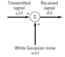
Figure7.1 AWGN moddel of a channel.

In minimizing the average probability of symbol error between the receiver output and the symbol emitted by the source, the motivation is to make the digital communication system as reliable as possible. To achieve this important design objective in a generic setting that involves an M-ary alphabet whose symbols are denoted by m₁, m₂,…,m_M, we have to understand two basic issues:

1.  How to optimize the design of the receiver so as to minimize the average probability of symbol error.

2.  How to choose the set of signals s₁(t), s₂(t), …, s_M(t) for representing the symbols m₁, m₂,…,m_M, respectively, since this choice affects the average probability of symbol error.

The key question is how to develop this understanding in a principled as well as insightful manner. The answer to this fundamental question is found in the geometric representation of signals.

7.2  Geometric Representation of Signals

The essence of geometric representation of signals¹ is to represent any set of M energy signals {s_i(t)} as linear combinations of N orthonormal basis functions, where N ≤ M. That is to say, given a set of real-valued energy signals, s₁(t), s₂(t),…,s_M(t), each of duration T seconds, we write

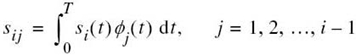
where the coefficients of the expansion are defined by

The real-valued basis functions ϕ₁(t), ϕ₂(t),…,ϕ_N(t) form an orthonormal set, by which we mean

where δ_ij is the Kronecker delta. The first condition of (7.6) states that each basis function is normalized to have unit energy. The second condition states that the basis functions ϕ₁(t), ϕ₂(t),…,ϕ_N(t) are orthogonal with respect to each other over the interval 0 ≤ t ≤ T.

For prescribed i, the set of coefficients may be viewed as an N-dimensional signal vector, denoted by s_i. The important point to note here is that the vector s_i bears a one-to-one relationship with the transmitted signal s_i(t):

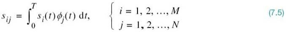
• Given the N elements of the vector s_i operating as input, we may use the scheme shown in Figure 7.2a to generate the signal s_i(t), which follows directly from (7.4). This figure consists of a bank of N multipliers with each multiplier having its own basis function followed by a summer. The scheme of Figure 7.2a may be viewed as a synthesizer.
• Conversely, given the signals s_i(t), i = 1,2,…,M, operating as input, we may use the scheme shown in Figure 7.2b to calculate the coefficients s_i1, s_i2, …, s_iN which follows directly from (7.5). This second scheme consists of a bank of N product-integrators or correlators with a common input, and with each one of them supplied with its own basis function. The scheme of Figure 7.2b may be viewed as an analyzer.

Figure 7.2, (a) Synthesizer for generating the signal s_i(t). (b) Analyzer for reconstructing the signal vector {s_i}.

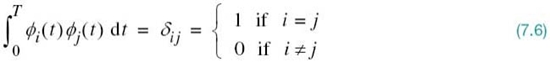
Figure 7.3 Illustrating the geometric representation of signals for the case when N = 2 and M = 3.

Accordingly, we may state that each signal in the set {s_i(t)} is completely determined by the signal vector

Furthermore, if we conceptually extend our conventional notion of two- and three-dimensional Euclidean spaces to an N-dimensional Euclidean space, we may visualize the set of signal vectors {s_i|i = 1,2,…,M} as defining a corresponding set of M points in an N-dimensional Euclidean space, with N mutually perpendicular axes labeled ϕ₁, ϕ₂,…,ϕ_N. This N-dimensional Euclidean space is called the signal space.

The idea of visualizing a set of energy signals geometrically, as just described, is of profound theoretical and practical importance. It provides the mathematical basis for the geometric representation of energy signals in a conceptually satisfying manner. This form of representation is illustrated in Figure 7.3 for the case of a two-dimensional signal space with three signals; that is, N = 2 and M = 3.

In an N-dimensional Euclidean space, we may define lengths of vectors and angles between vectors. It is customary to denote the length (also called the absolute value or norm) of a signal vector s_i by the symbol ||s_i||. The squared length of any signal vector s_i is defined to be the inner product or dot product of s_i with itself, as shown by

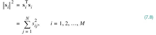
where s_ij is the jth element of s_i and the superscript T denotes matrix transposition.

There is an interesting relationship between the energy content of a signal and its representation as a vector. By definition, the energy of a signal s_i(t) of duration T seconds is

Therefore, substituting (7.4) into (7.9), we get

Interchanging the order of summation and integration, which we can do because they are both linear operations, and then rearranging terms we get

Since, by definition, the ϕ_j(t) form an orthonormal set in accordance with the two conditions of (7.6), we find that (7.10) reduces simply to

Thus, (7.8) and (7.11) show that the energy of an energy signal s_i(t) is equal to the squared length of the corresponding signal vector s_i(t).

In the case of a pair of signals s_i(t) and s_k(t) represented by the signal vectors s_i and s_k, respectively, we may also show that

Equation (7.12) states:

The inner product of the energy signals s_i(t) and s_k(t) over the interval [0, T] is equal to the inner product of their respective vector representations s_i and s_k.

Note that the inner product is invariant to the choice of basis functions , in that it only depends on the components of the signals s_i(t) and s_k(t) projected onto each of the basis functions.

Yet another useful relation involving the vector representations of the energy signals s_i(t) and s_k(t) is described by

where is the Euclidean distance d_ik between the points represented by the signal vectors s_i and s_k.

To complete the geometric representation of energy signals, we need to have a representation for the angle θ_ik subtended between two signal vectors s_i and s_k. By definition, the cosine of the angle θ_ik is equal to the inner product of these two vectors divided by the product of their individual norms, as shown by

The two vectors s_i and s_k are thus orthogonal or perpendicular to each other if their inner product | is zero, in which case θ_ik = 90°; this condition is intuitively satisfying.

EXAMPLE 1   The Schwarz Inequality

Consider any pair of energy signals s₁(t) and s₂(t). The Schwarz inequality states

The equality holds if, and only if, s₂(t) = cs₁(t), where c is any constant.

To prove this important inequality, let s₁(t) and s₂(t) be expressed in terms of the pair of orthonormal basis functions ϕ₁(t) and ϕ₂(t) as follows:

where ϕ₁(t) and ϕ₂(t) satisfy the orthonormality conditions over the time interval (–∞, ∞):

On this basis, we may represent the signals s₁(t) and s₂(t) by the following respective pair of vectors, as illustrated in Figure 7.4:

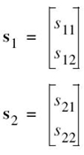
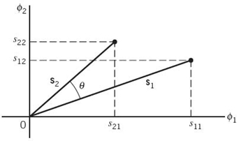
Figure 7.4 Vector representations of signals s₁(t) and s₂(t), providing the background picture for proving the Schwarz inequality.

From Figure 7.4 we readily see that the cosine of angle θ subtended between the vectors s₁ and s₂ is

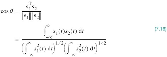
where we have made use of (7.14) and (7.12). Recognizing that |cosθ | ≤ 1, the Schwarz inequality of (7.15) immediately follows from (7.16). Moreover, from the first line of (7.16) we note that |cosθ | = 1 if, and only if, s₂ = cs₁; that is, s₂(t) = cs₁(t), where c is an arbitrary constant.

Proof of the Schwarz inequality, as presented here, applies to real-valued signals. It may be readily extended to complex-valued signals, in which case (7.15) is reformulated as

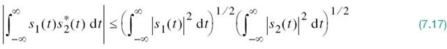
where the asterisk denotes complex conjugation and the equality holds if, and only if, s₂(t) = cs₁(t), where c is a constant.

 Gram–Schmidt Orthogonalization Procedure

Having demonstrated the elegance of the geometric representation of energy signals with an example, how do we justify it in mathematical terms? The answer to this question lies in the Gram–Schmidt orthogonalization procedure, for which we need a complete orthonormal set of basis functions. To proceed with the formulation of this procedure, suppose we have a set of M energy signals denoted by s₁(t), s₂(t),…,s_M(t). Starting with s₁(t) chosen from this set arbitrarily, the first basis function is defined by

where E₁ is the energy of the signal s₁(t).

Then, clearly, we have

where the coefficient and ϕ₁(t) has unit energy as required.

Next, using the signal s₂(t), we define the coefficient s₂₁ as

We may thus introduce a new intermediate function

which is orthogonal to ϕ₁(t) over the interval 0 ≤ t ≤ T by virtue of the definition of s₂₁ and the fact that the basis function ϕ₁(t) has unit energy. Now, we are ready to define the second basis function as

Substituting (7.19) into (7.20) and simplifying, we get the desired result

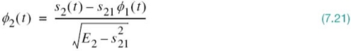
where E₂ is the energy of the signal s₂(t). From (7.20) we readily see that

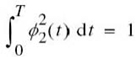
in which case (7.21) yields

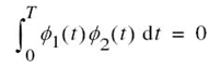
That is to say, ϕ₁(t) and ϕ₂(t) form an orthonormal pair as required.

Continuing the procedure in this fashion, we may, in general, define

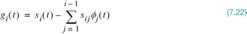
where the coefficients s_ij are themselves defined by

For i = 1, the function g_i(t) reduces to s_i(t).

Given the g_i(t), we may now define the set of basis functions

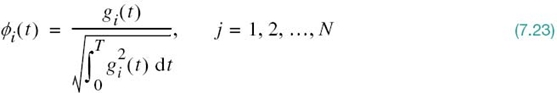
which form an orthonormal set. The dimension N is less than or equal to the number of given signals, M, depending on one of two possibilities:

• The signals s₁(t), s₂(t),…,s_M(t) form a linearly independent set, in which case N = M.
• The signals s₁(t), s₂(t),…,s_M(t) are not linearly independent, in which case N < M and the intermediate function g_i(t) is zero for i > N.

Note that the conventional Fourier series expansion of a periodic signal, discussed in Chapter 2, may be viewed as a special case of the Gram–Schmidt orthogonalization procedure. Moreover, the representation of a band-limited signal in terms of its samples taken at the Nyquist rate, discussed in Chapter 6, may be viewed as another special case. However, in saying what we have here, two important distinctions should be made:

1.  The form of the basis functions ϕ₁(t), ϕ₂(t),…,ϕ_N(t) has not been specified. That is to say, unlike the Fourier series expansion of a periodic signal or the sampled representation of a band-limited signal, we have not restricted the Gram–Schmidt orthogonalization procedure to be in terms of sinusoidal functions (as in the Fourier series) or sinc functions of time (as in the sampling process).

2.   The expansion of the signal s_i(t) in terms of a finite number of terms is not an approximation wherein only the first N terms are significant; rather, it is an exact expression, where N and only N terms are significant.

EXAMPLE 2  2B1Q Code

The 2B1Q code is the North American line code for a special class of modems called digital subscriber lines. This code represents a quaternary PAM signal as shown in the Gray-encoded alphabet of Table 7.1. The four possible signals s₁(t), s₂(t), s₃(t), and s₄(t) are amplitude-scaled versions of a Nyquist pulse. Each signal represents a dibit (i.e., pair of bits). The issue of interest is to find the vector representation of the 2B1Q code.

This example is simple enough for us to solve it by inspection. Let ϕ₁(t) denote a pulse normalized to have unit energy. The ϕ₁(t) so defined is the only basis function for the vector representation of the 2B1Q code. Accordingly, the signal-space representation of this code is as shown in Figure 7.5. It consists of four signal vectors s₁, s₂, s₃, and s₄, which are located on the ϕ₁-axis in a symmetric manner about the origin. In this example, we have M = 4 and N = 1.

Table 7.1 Amplitude levels of the 2B1Q code

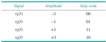
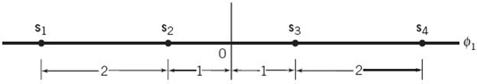
Figure 7.5 Signal-space representation of the 2B1Q code.

We may generalize the result depicted in Figure 7.5 for the 2B1Q code as follows: the signal-space diagram of an M-ary PAM signal, in general, is one-dimensional with M signal points uniformly positioned on the only axis of the diagram.

7.3  Conversion of the Continuous AWGN Channel into a Vector Channel

Suppose that the input to the bank of N product integrators or correlators in Figure 7.2b, is not the transmitted signal s_i(t) but rather the received signal x(t) defined in accordance with the AWGN channel of Figure 7.1. That is to say,

where w(t) is a sample function of the white Gaussian noise process W(t) of zero mean and power spectral density N₀/2. Correspondingly, we find that the output of correlator j, say, is the sample value of a random variable X_j, whose sample value is defined by

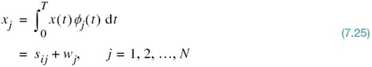
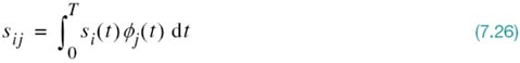
The first component, s_ij, is the deterministic component of x_j due to the transmitted signal s_i(t), as shown by

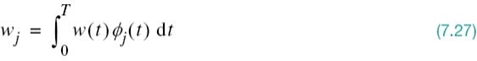
The second component, w_j, is the sample value of a random variable W_j due to the channel noise w(t), as shown by

Consider next a new stochastic process X' (t) whose sample function x' (t) is related to the received signal x(t) as follows:

Substituting (7.24) and (7.25) into (7.28), and then using the expansion of (7.4), we get

The sample function x' (t), therefore, depends solely on the channel noise w(t). On the basis of (7.28) and (7.29), we may thus express the received signal as

Accordingly, we may view w'(t) as a remainder term that must be included on the right-hand side of (7.30) to preserve equality. It is informative to contrast the expansion of the received signal x(t) given in (7.30) with the corresponding expansion of the transmitted signal s_i(t) given in (7.4): the expansion of (7.4), pertaining to the transmitter, is entirely deterministic; on the other hand, the expansion of (7.30) is random (stochastic) due to the channel noise at the receiver input.

Statistical Characterization of the Correlator Outputs

We now wish to develop a statistical characterization of the set of N correlator outputs. Let X(t) denote the stochastic process, a sample function of which is represented by the received signal x(t). Correspondingly, let X_j denote the random variable whose sample value is represented by the correlator output x_j, j = 1,2,…,N. According to the AWGN model of Figure 7.1, the stochastic process X(t) is a Gaussian process. It follows, therefore, that X_j is a Gaussian random variable for all j in accordance with Property 1 of a Gaussian process (Chapter 4). Hence, X_j is characterized completely by its mean and variance, which are determined next.

Let W_j denote the random variable represented by the sample value w_j produced by the jth correlator in response to the white Gaussian noise component w(t). The random variable W_j has zero mean because the channel noise process W(t) represented by w(t) in the AWGN model of Figure 7.1 has zero mean by definition. Consequently, the mean of X_j depends only on s_ij, as shown by

To find the variance of X_j, we start with the definition

where the last line follows from (7.25) with x_j and w_j replaced by X_j and W_j, respectively. According to (7.27), the random variable W_j is defined by

We may therefore expand (7.32) as

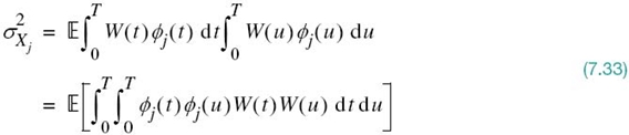
Interchanging the order of integration and expectation, which we can do because they are both linear operations, we obtain

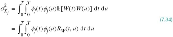
where R_W(t, u) is the autocorrelation function of the noise process W(t). Since this noise is stationary, R_W(t, u) depends only on the time difference t – u. Furthermore, since W(t) is white with a constant power spectral density N₀/2, we may express R_W(t, u) as

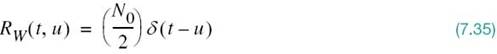
Therefore, substituting (7.35) into (7.34) and then using the sifting property of the delta function δ(t), we get

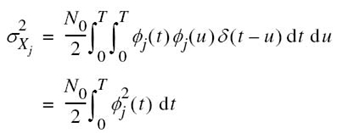
Since the ϕ_j(t) have unit energy, by definition, the expression for noise variance reduces to

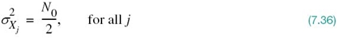
This important result shows that all the correlator outputs, denoted by X_j with j = 1,2,…,N, have a variance equal to the power spectral density N₀/2 of the noise process W(t).

Moreover, since the basic functions ϕ_j(t) form an orthonormal set, X_j and X_k are mutually uncorrelated, as shown by

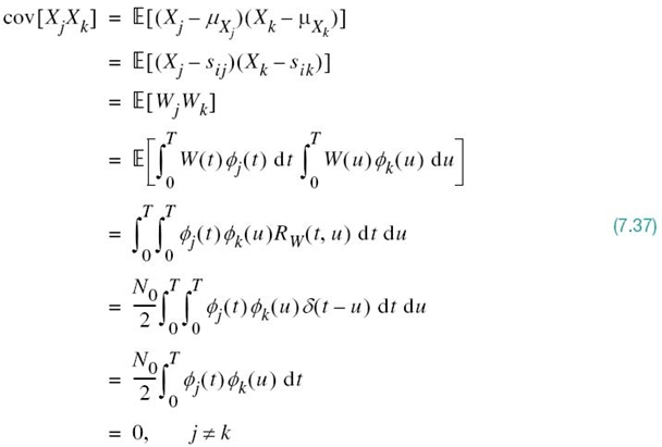
Since the X_j are Gaussian random variables, (7.37) implies that they are also statistically independent in accordance with Property 4 of a Gaussian process (Chapter 4).

Define the vector of N random variables

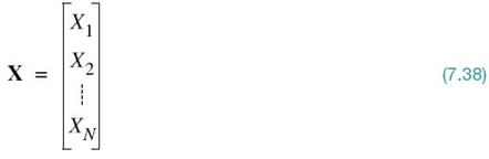
whose elements are independent Gaussian random variables with mean values equal to s_ij and variances equal to N₀/2. Since the elements of the vector X are statistically independent, we may express the conditional probability density function of the vector X, given that the signal s_i(t) or the corresponding symbol m_i was sent, as the product of the conditional probability density functions of its individual elements; that is,

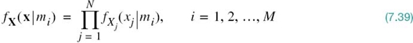
where the vector x and scalar x_j are sample values of the random vector X and random variable X_j, respectively. The vector x is called the observation vector; correspondingly, x_j is called an element of the observation vector. A channel that satisfies (7.39) is said to be a memoryless channel.

Since each X_j is a Gaussian random variable with mean s_ij and variance N₀/2, we have

Therefore, substituting (7.40) into (7.39) yields

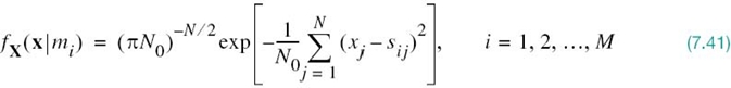
which completely characterizes the first term of (7.30).

However, there remains the noise term w'(t) in (7.30) to be accounted for. Since the noise process W(t) represented by w(t) is Gaussian with zero mean, it follows that the noise process W'(t) represented by the sample function w'(t) is also a zero-mean Gaussian process. Finally, we note that any random variable W'(t_k), say, derived from the noise process W'(t) by sampling it at time t_k, is in fact statistically independent of the random variable X_j; that is to say:

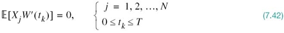
Since any random variable based on the remainder noise W'(t) process is independent of the set of random variables {X_j} as well as the set of transmitted signals {s_i(t)}, (7.42) states that the random variable W'(t_k) is irrelevant to the decision as to which particular signal was actually transmitted. In other words, the correlator outputs determined by the received signal x(t) are the only data that are useful for the decision-making process; therefore, they represent sufficient statistics for the problem at hand. By definition, sufficient statistics summarize the whole of the relevant information supplied by an observation vector.

We may now summarize the results presented in this section by formulating the theorem of irrelevance:

Insofar as signal detection in AWGN is concerned, only the projections of the noise onto the basis functions of the signal set affect the sufficient statistics of the detection problem; the remainder of the noise is irrelevant.

Putting this theorem into a mathematical context, we may say that the AWGN channel model of Figure 7.1a is equivalent to an N-dimensional vector channel described by the equation

where the dimension N is the number of basis functions involved in formulating the signal vector s_i for all i. The individual components of the signal vector s_i and the additive Gaussian noise vector w are defined by (7.5) and (7.27), respectively. The theorem of irrelevance and its mathematical description given in (7.43) are indeed basic to the understanding of the signal-detection problem as described next. Just as importantly, (7.43) may be viewed as the baseband version of the time-dependent received signal of (7.24).

Likelihood Function

The conditional probability density functions f_X(x|m_i),  i = 1,2,…,M, provide the very characterization of an AWGN channel. Their derivation leads to a functional dependence on the observation vector x given the transmitted message symbol m_i. However, at the receiver we have the exact opposite situation: we are given the observation vector x and the requirement is to estimate the message symbol m_i that is responsible for generating x. To emphasize this latter viewpoint, we follow Chapter 3 by introducing the idea of a likelihood function, denoted by L(m_i) and defined by

However, tt is important to recall from Chapter 3 that although l(m_i) and f_X(x|m_i) have exactly the same mathematical form, their individual meanings are quite different.

In practice, we find it more convenient to work with the log-likelihood function, denoted by L(m_i) and defined by

where ln denotes the natural logarithm. The log-likelihood function bears a one-to-one relationship to the likelihood function for two reasons:

1.   By definition, a probability density function is always nonnegative. It follows, therefore, that the likelihood function is likewise a nonnegative quantity.

2.  The logarithmic function is a monotonically increasing function of its argument.

The use of (7.41) in (7.45) yields the log-likelihood function for an AWGN channel as

where we have ignored the constant term –(N/2)ln(πN₀) since it bears no relation whatsoever to the message symbol m_i. Recall that the s_ij, j = 1,2,…,N, are the elements of the signal vector s_i representing the message symbol m_i. With (7.46) at our disposal, we re now ready to address the basic receiver design problem.

7.4   Optimum Receivers Using Coherent Detection

Maximum Likelihood Decoding

Suppose that, in each time slot of duration T seconds, one of the M possible signals s₁(t), s₂(t),…,s_M(t) is transmitted with equal probability, 1/M. For geometric signal representation, the signal s_i(t), i = 1,2,…,M, is applied to a bank of correlators with a common input and supplied with an appropriate set of N orthonormal basis functions, as depicted in Figure 7.2b. The resulting correlator outputs define the signal vector s_i. Since knowledge of the signal vector s_i is as good as knowing the transmitted signal s_i(t) itself, and vice versa, we may represent s_i(t) by a point in a Euclidean space of dimension N ≤ M. We refer to this point as the transmitted signal point, or message point for short. The set of message points corresponding to the set of transmitted signals is called a message constellation.

However, representation of the received signal x(t) is complicated by the presence of additive noise w(t). We note that when the received signal x(t) is applied to the bank of N correlators, the correlator outputs define the observation vector x. According to (7.43), the vector x differs from the signal vector s_i by the noise vector w, whose orientation is completely random, as it should be.

The noise vector w is completely characterized by the channel noise w(t); the converse of this statement, however, is not true, as explained previously. The noise vector w represents that portion of the noise w(t) that will interfere with the detection process; the remaining portion of this noise, denoted by w'(t), is tuned out by the bank of correlators and, therefore, irrelevant.

Based on the observation vector x, we may represent the received signal x(t) by a point in the same Euclidean space used to represent the transmitted signal. We refer to this second point as the received signal point. Owing to the presence of noise, the received signal point wanders about the message point in a completely random fashion, in the sense that it may lie anywhere inside a Gaussian-distributed “cloud” centered on the message point. This is illustrated in Figure 7.6a for the case of a three-dimensional signal space. For a particular realization of the noise vector w (i.e., a particular point inside the random cloud of Figure 7.6a) the relationship between the observation vector x and the signal vector s_i is as illustrated in Figure 7.6b.

We are now ready to state the signal-detection problem:

Given the observation vector x, perform a mapping from x to an estimate m̂ of the transmitted symbol, m_i, in a way that would minimize the probability of error in the decision-making process.

Given the observation vector x, suppose that we make the decision m̂ = m_i. The probability of error in this decision, which we denote by P_e(m_i|x), is simply

The requirement is to minimize the average probability of error in mapping each given observation vector x into a decision. On the basis of (7.47), we may, therefore, state the optimum decision rule:

The decision rule described in (7.48) is referred to as the maximum a posteriori probability (MAP) rule. Correspondingly, the system used to implement this rule is called a maximum a posteriori decoder.

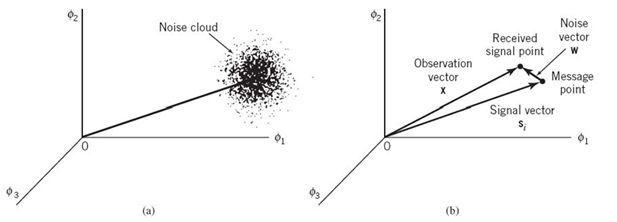
Figure 7.6 Illustrating the effect of (a) noise perturbation on (b) the location of the received signal point.

The requirement of (7.48) may be expressed more explicitly in terms of the prior probabilities of the transmitted signals and the likelihood functions, using Bayes’ rule discussed in Chapter 3. For the moment, ignoring possible ties in the decision-making process, we may restate the MAP rule as follows:

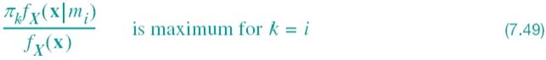
where π_k is the prior probability of transmitting symbol m_k, f_X(x|m_i) is the conditional probability density function of the random observation vector X given the transmission of symbol m_k, and f_X(x) is the unconditional probability density function of X.

In (7.49), we now note the following points:

• the denominator term f_X(x) is independent of the transmitted symbol;
• the prior probability π_k = π_i when all the source symbols are transmitted with equal probability; and
• the conditional probability density function f_X(x|m_k) bears a one-to-one relationship to the log-likelihood function L(m_k).

Accordingly, we may simply restate the decision rule of (7.49) in terms of L(m_k) as follows:

The decision rule of (7.50) is known as the maximum likelihood rule, discussed previously in Chapter 3; the system used for its implementation is correspondingly referred to as the maximum likelihood decoder. According to this decision rule, a maximum likelihood decoder computes the log-likelihood functions as metrics for all the M possible message symbols, compares them, and then decides in favor of the maximum. Thus, the maximum likelihood decoder is a simplified version of the maximum a posteriori decoder, in that the M message symbols are assumed to be equally likely.

It is useful to have a graphical interpretation of the maximum likelihood decision rule. Let Z denote the N-dimensional space of all possible observation vectors x. We refer to this space as the observation space. Because we have assumed that the decision rule must say m̂ = m_i, where i = 1,2,…,M, the total observation space Z is correspondingly partitioned into M-decision regions, denoted by Z₁,Z₂,…,Z_M. Accordingly, we may restate the decision rule of (7.50) as

Aside from the boundaries between the decision regions Z₁,Z₂,…,Z_M, it is clear that this set of regions covers the entire observation space. We now adopt the convention that all ties are resolved at random; that is, the receiver simply makes a random guess. Specifically, if the observation vector x falls on the boundary between any two decision regions, Z_i and Z_k, say, the choice between the two possible decisions m̂ = m_k and m̂ = m_i is resolved a priori by the flip of a fair coin. Clearly, the outcome of such an event does not affect the ultimate value of the probability of error since, on this boundary, the condition of (7.48) is satisfied with the equality sign.

The maximum likelihood decision rule of (7.50) or its geometric counterpart described in (7.51) assumes that the channel noise w(t) is additive. We next specialize this rule for the case when w(t) is both white and Gaussian.

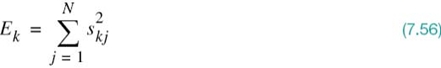
From the log-likelihood function defined in (7.46) for an AWGN channel, we note that

L(m_k) attains its maximum value when the summation term is minimized by the choice k = i. Accordingly, we may formulate the maximum likelihood decision rule for an AWGN channel as

Note we have used “minimum” as the optimizing condition in (7.52) because the minus sign in (7.46) has been ignored. Next, we note from the discussion presented in Section 7.2 that

where ||x–s_k|| is the Euclidean distance between the observation vector x at the receiver input and the transmitted signal vector s_k. Accordingly, we may restate the decision rule of (7.53) as

In words, (7.54) states that the maximum likelihood decision rule is simply to choose the message point closest to the received signal point, which is intuitively satisfying.

In practice, the decision rule of (7.54) is simplified by expanding the summation on the left-hand side of (7.53) as

The first summation term of this expansion is independent of the index k pertaining to the transmitted signal vector s_k and, therefore, may be ignored. The second summation term is the inner product of the observation vector x and the transmitted signal vector s_k. The third summation term is the transmitted signal energy

Accordingly, we may reformulate the maximum-likelihood decision rule one last time:

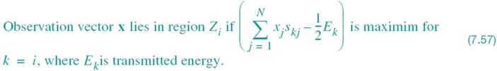
Figure 7.7 Illustrating the partitioning of the observation space into decision regions for the case when N = 2 and M = 4; it is assumed that the M transmitted symbols are equally likely.

From (7.57) we infer that, for an AWGN channel, the M decision regions are bounded by linear hyperplane boundaries. The example in Figure 7.7 illustrates this statement for M = 4 signals and N = 2 dimensions, assuming that the signals are transmitted with equal energy E and equal probability.

Correlation Receiver

In light of the material just presented, the optimum receiver for an AWGN channel and for the case when the transmitted signals s₁(t), s₂(t),…,s_M(t) are equally likely is called a correlation receiver; it consists of two subsystems, which are detailed in Figure 7.8:

1.  Detector (Figure 7.8a), which consists of M correlators supplied with a set of orthonormal basis functions ϕ₁(t), ϕ₂(t),…,ϕ_N(t) that are generated locally; this bank of correlators operates on the received signal x(t), 0 ≤ t ≤ T, to produce the observation vector x.

2.  Maximum-likelihood decoder (Figure 7.8b), which operates on the observation vector x to produce an estimate m̂ of the transmitted symbol m_i, i = 1,2,…,M, in such a way that the average probability of symbol error is minimized.

In accordance with the maximum likelihood decision rule of (7.57), the decoder multiplies the N elements of the observation vector x by the corresponding N elements of each of the M signal vectors s₁, s₂,…, s_M. Then, the resulting products are successively summed in accumulators to form the corresponding set of inner products {x^Ts_k|k = 1,2,…,M}.

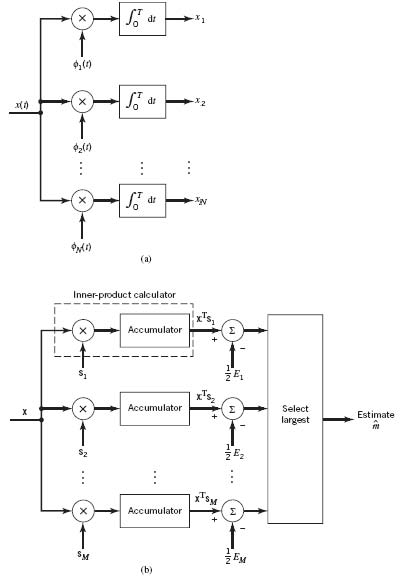
Figure 7.8 (a) Detector or demodulator. (b) Signal transmission decoder.

Next, the inner products are corrected for the fact that the transmitted signal energies may be unequal. Finally, the largest one in the resulting set of numbers is selected, and an appropriate decision on the transmitted message is thereby made.

Matched Filter Receiver

The detector shown in Figure 7.8a involves a set of correlators. Alternatively, we may use a different but equivalent structure in place of the correlators. To explore this alternative method of implementing the optimum receiver, consider a linear time-invariant filter with impulse response h_j(t). With the received signal x(t) operating as input, the resulting filter output is defined by the convolution integral

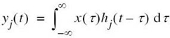
To proceed further, we evaluate this integral over the duration of a transmitted symbol, namely 0 ≤ t ≤ T. With time t restricted in this manner, we may replace the variable τ with t and go on to write

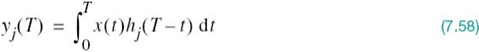
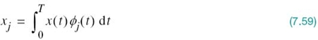
Consider next a detector based on a bank of correlators. The output of the jth correlator is defined by the first line of (7.25), reproduced here for convenience of representation:

For y_j(T) to equal x_j, we find from (7.58) and (7.59) that this condition is satisfied provided that we choose

Equivalently, we may express the condition imposed on the desired impulse response of the filter as

We may now generalize the condition described in (7.60) by stating:

Given a pulse signal ϕ(t) occupying the interval 0 ≤ t ≤ T, a linear time-invariant filter is said to be matched to the signal ϕ(t) if its impulse response h(t) satisfies the condition

A time-invariant filter defined in this way is called a matched filter. Correspondingly, an optimum receiver using matched filters in place of correlators is called a matched-filter receiver. Such a receiver is depicted in Figure 7.9, shown below.

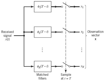
Figure 7.9 Detector part of matched filter receiver; the signal transmission decoder is as shown in Figure 7.8(b).

7.5    Probability of Error

To complete the statistical characterization of the correlation receiver of Figure 7.8a or its equivalent, the matched filter receiver of Figure 7.9, we need to evaluate its performance in the presence of AWGN. To do so, suppose that the observation space Z is partitioned into a set of regions, , in accordance with the maximum likelihood decision rule. Suppose also that symbol m_i (or, equivalently, signal vector s_i) is transmitted and an observation vector x is received. Then, an error occurs whenever the received signal point represented by x does not fall inside region Z_i associated with the message point s_i. Averaging over all possible transmitted symbols assumed to be equiprobable, we see that the average probability of symbol error is

where we have used the standard notation to denote the conditional probability of an event. Since x is the sample value of random vector X, we may rewrite (7.62) in terms of the likelihood function as follows, given that the message symbol m_i is sent:

For an N-dimensional observation vector, the integral in (7.63) is likewise N-dimensional.

Invariance of the Probability of Error to Rotation

There is a uniqueness to the way in which the observation space Z is partitioned into the set of regions Z₁,Z₂, …, Z_M in accordance with the maximum likelihood detection of a signal in AWGN; that uniqueness is defined by the message constellation under study. In particular, we may make the statement:

Changes in the orientation of the message constellation with respect to both the coordinate axes and origin of the signal space do not affect the probability of symbol error P_e defined in (7.63).

This statement embodies the invariance property of the average probability of symbol error P_e with respect to notation and translation, which is the result of two facts:

1.  In maximum likelihood detection, the probability of symbol error P_e depends solely on the relative Euclidean distance between a received signal point and message point in the constellation.

2.  The AWGN is spherically symmetric in all directions in the signal space.

To elaborate, consider first the invariance of P_e with respect to rotation. The effect of a rotation applied to all the message points in a constellation is equivalent to multiplying the N-dimensional signal vector s_i by an N-by-N orthonormal matrix denoted by Q for all i. By definition, the matrix Q satisfies the condition

where the superscript T denotes matrix transposition and I is the identity matrix whose diagonal elements are all unity and its off-diagonal elements are all zero. According to (7.64), the inverse of the real-valued orthonormal matrix Q is equal to its own transpose. Thus, in dealing with rotation, the message vector s_i is replaced by its rotated version

Correspondingly, the N-by-1 noise vector w is replaced by its rotated version

However, the statistical characteristics of the noise vector are unaffected by this rotation for three reasons:

1.  From Chapter 4 we recall that a linear combination of Gaussian random variables is also Gaussian. Since the noise vector w is Gaussian, by assumption, then it follows that the rotated noise vector w_rotate is also Gaussian.

2.  Since the noise vector w has zero mean, the rotated noise vector w_rotate also has zero mean, as shown by

3.  The covariance matrix of the noise vector w is equal to (N₀/2)I, where N₀/2 is the power spectral density of the AWGN w(t) and I is the identity matrix; that is

Hence, the covariance matrix of the rotated noise vector is

where, in the last two lines, we have made use of (7.68) and (7.64).

In light of these three reasons, we may, therefore, express the observation vector in the rotated message constellation as

Using (7.65) and (7.70), we may now express the Euclidean distance between the rotated vectors x_rotate and s_rotate as

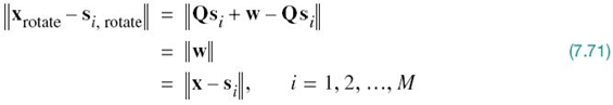
where, in the last line, we made use of (7.43).

We may, therefore, formally state the principle of rotational invariance:

If a message constellation is rotated by the transformation

where Q is an orthonormal matrix, then the probability of symbol error P_e incurred in maximum likelihood signal-detection over an AWGN channel is completely unchanged.

EXAMPLE 3   Illustration of Rotational Invariance

To illustrate the principle of rotational invariance, consider the signal constellation shown in Figure 7.10a. The constellation is the same as that of Figure 7.10b, except for the fact that it has been rotated through 45°. Although these two constellations do indeed look different in a geometric sense, the principle of rotational invariance teaches us immediately that the P_e is the same for both of them.

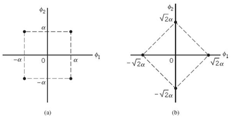
Figure 7.10 A pair of signal constellations for illustrating the principle of rotational invariance.

Invariance of the Probability to Translation

Consider next the invariance of P_e to translation. Suppose all the message points in a signal constellation are translated by a constant vector amount a, as shown by

The observation vector is correspondingly translated by the same vector amount, as shown by

From (7.72) and (7.73) we see that the translation a is common to both the translated signal vector s_i and translated observation vector x. We, therefore, immediately deduce that

and thus formulate the principle of translational invariance:

If a signal constellation is translated by a constant vector amount, then the probability of symbol error P_e incurred in maximum likelihood signal detection over an AWGN channel is completely unchanged.

EXAMPLE 4   Translation of Signal Constellation

As an example, consider the two signal constellations shown in Figure 7.11, which pertain to a pair of different four-level PAM signals. The constellation of Figure 7.11b is the same as that of Figure 7.11a, except for a translation 3 α/2 to the right along the ϕ₁-axis. The principle of translational invariance teaches us that the P_e is the same for both of these signal constellations.

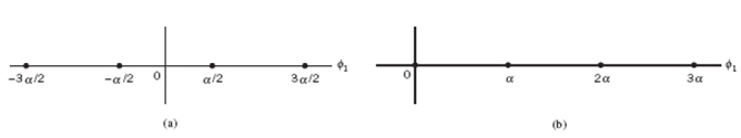
Figure 7.11 A pair of signal constellations for illustrating the principle of translational invariance.

Union Bound on the Probability of Error

For AWGN channels, the formulation of the average probability of symbol error ² P_e is conceptually straightforward, in that we simply substitute (7.41) into (7.63). Unfortunately, however, numerical computation of the integral so obtained is impractical, except in a few simple (nevertheless, important) cases. To overcome this computational difficulty, we may resort to the use of bounds, which are usually adequate to predict the SNR (within a decibel or so) required to maintain a prescribed error rate. The approximation to the integral defining P_e is made by simplifying the integral or simplifying the region of integration. In the following, we use the latter procedure to develop a simple yet useful upper bound, called the union bound, as an approximation to the average probability of symbol error for a set of M equally likely signals (symbols) in an AWGN channel.

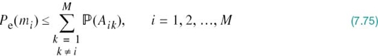
Let A_ik, with (i, k) = 1,2,…,M, denote the event that the observation vector x is closer to the signal vector s_k than to s_i, when the symbol m_i (message vector s_i) is sent. The conditional probability of symbol error when symbol m_i is sent, P_e(m_i), is equal to the probability of the union of events, defined by the set . Probability theory teaches us that the probability of a finite union of events is overbounded by the sum of the probabilities of the constituent events. We may, therefore, write

EXAMPLE 5   Constellation of Four Message Points

To illustrate applicability of the union bound, consider Figure 7.12 for the case of M = 4. Figure 7.12a shows the four message points and associated decision regions, with the point s₁ assumed to represent a transmitted symbol. Figure 7.12b shows the three constituent signal-space descriptions where, in each case, the transmitted message point s₁ and one other message point are retained. According to Figure 7.12a the conditional probability of symbol error, P_e(m_i), is equal to the probability that the observation vector x lies in the shaded region of the two-dimensional signal-space diagram. Clearly, this probability is less than the sum of the probabilities of the three individual events that x lies in the shaded regions of the three constituent signal spaces depicted in Figure 7.12b.

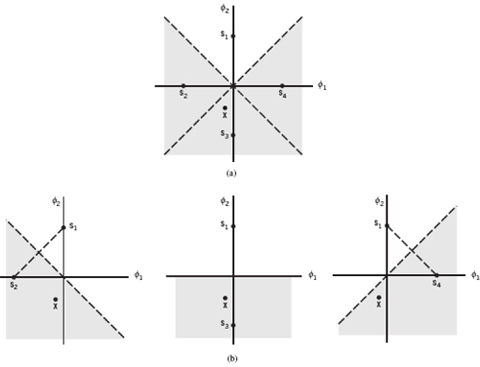
Figure 7.12 Illustrating the union bound. (a) Constellation of four message points. (b) Three constellations with a common message point and one other message point x retained from the original constellation.

Pairwise Error Probability

It is important to note that, in general, the probability is different from the probability , which is the probability that the observation vector x is closer to the signal vector s_k (i.e., symbol m_k) than every other when the vector s_i (i.e., symbol m_i) is sent. On the other hand, the probability depends on only two signal vectors, s_i and s_k. To emphasize this difference, we rewrite (7.75) by adopting p_ik in place of . We thus write

The probability p_ik is called the pairwise error probability, in that if a digital communication system uses only a pair of signals, s_i and s_k, then p_ik is the probability of the receiver mistaking s_k for s_i.

Consider then a simplified digital communication system that involves the use of two equally likely messages represented by the vectors s_i and s_k. Since white Gaussian noise is identically distributed along any set of orthogonal axes, we may temporarily choose the first axis in such a set as one that passes through the points s_i and s_k; for three illustrative examples, see Figure 7.12b. The corresponding decision boundary is represented by the bisector that is perpendicular to the line joining the points s_i and s_k. Accordingly, when the vector s_i (i.e., symbol m_i) is sent, and if the observation vector x lies on the side of the bisector where s_k lies, an error is made. The probability of this event is given by

where d_ik in the lower limit of the integral is the Euclidean distance between signal vectors s_i and s_k; that is,

To change the integral of (7.77) into a standard form, define a new integration variable

Equation (7.77) is then rewritten in the desired form

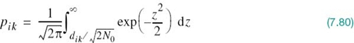
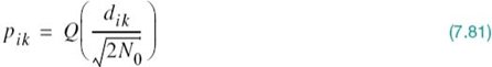
The integral in (7.80) is the Q-function of (3.68) that was introduced in Chapter 3. In terms of the Q-function, we may now express the probability p_ik in the compact form

Correspondingly, substituting (7.81) into (7.76), we write

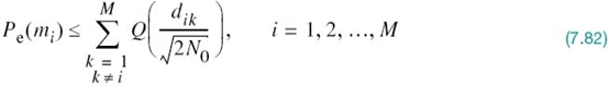
The probability of symbol error, averaged over all the M symbols, is, therefore, over-bounded as follows:

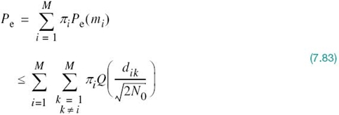
where π_i is the probability of sending symbol m_i.

There are two special forms of (7.83) that are noteworthy:

1.  Suppose that the signal constellation is circularly symmetric about the origin. Then, the conditional probability of error P_e(m_i) is the same for all i, in which case (7.83) reduces to

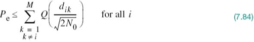
Figure 7.10 illustrates two examples of circularly symmetric signal constellations.

2.  Define the minimum distance of a signal constellation d_min as the smallest Euclidean distance between any two transmitted signal points in the constellation, as shown by

Then, recognizing that the Q-function is a monotonically decreasing function of its argument, we have

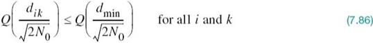
Therefore, in general, we may simplify the bound on the average probability of symbol error in (7.83) as

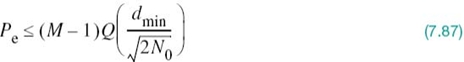
The Q-function in (7.87) is itself upper bounded as³

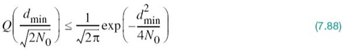
Accordingly, we may further simplify the bound on P_e in (7.87) as

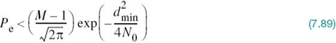
In words, (7.89) states the following:

In an AWGN channel, the average probability of symbol error P_e decreases exponentially as the squared minimum distance, d²_min.

Bit Versus Symbol Error Probabilities

Thus far, the only figure of merit we have used to assess the noise performance of a digital communication system in AWGN has been the average probability of symbol (word) error. This figure of merit is the natural choice when messages of length m = log₂ M are transmitted, such as alphanumeric symbols. However, when the requirement is to transmit binary data such as digital computer data, it is often more meaningful to use another figure of merit called the BER. Although, in general, there are no unique relationships between these two figures of merit, it is fortunate that such relationships can be derived for two cases of practical interest, as discussed next.

Case 1:   M-tuples Differing in Only a Single Bit

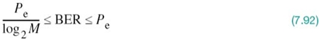
Suppose that it is possible to perform the mapping from binary to M-ary symbols in such a way that the two binary M-tuples corresponding to any pair of adjacent symbols in the M-ary modulation scheme differ in only one bit position. This mapping constraint is satisfied by using a Gray code. When the probability of symbol error P_e is acceptably small, we find that the probability of mistaking one symbol for either one of the two “nearest” symbols is greater than any other kind of symbol error. Moreover, given a symbol error, the most probable number of bit errors is one, subject to the aforementioned mapping constraint. Since there are log₂M bits per symbol, it follows that the average probability of symbol error is related to the BER as follows:

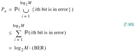
where, in the first line, ⋃ is the symbol for “union” as used in set theory. We also note that

It follows, therefore, that the BER is bounded as follows:

Case 2:   Number of Symbols Equal to Integer Power of 2

Suppose next M = 2^K, where K is an integer. We assume that all symbol errors are equally likely and occur with probability

where P_e is the average probability of symbol error. To find the probability that the ith bit in a symbol is in error, we note that there are 2^{K – 1} cases of symbol error in which this particular bit is changed and there are 2^{K – 1} cases in which it is not. Hence, the BER is

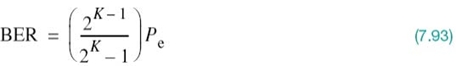
or, equivalently,

Note that, for large M, the BER approaches the limiting value of P_e/2. Note also that the bit errors are not independent in general.

7.6   Phase-Shift Keying Techniques Using Coherent Detection

With the background material on the coherent detection of signals in AWGN presented in Sections 7.2–7.4 at our disposal, we are now ready to study specific passband data-transmission systems. In this section, we focus on the family of phase-shift keying (PSK) techniques, starting with the simplest member of the family discussed next.

Binary Phase-Shift Keying

In a binary PSK system, the pair of signals s₁(t) and s₂(t) used to represent binary symbols 1 and 0, respectively, is defined by

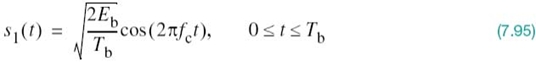
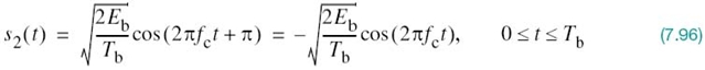
where T_b is the bit duration and E_b is the transmitted signal energy per bit. We find it convenient, although not necessary, to assume that each transmitted bit contains an integral number of cycles of the carrier wave; that is, the carrier frequency f_c is chosen equal to n_c/T_b for some fixed integer n_c. A pair of sinusoidal waves that differ only in a relative phase-shift of 180°, defined in (7.95) and (7.96), is referred to as an antipodal signal.

Signal-Space Diagram of Binary PSK Signals

From this pair of equations it is clear that, in the case of binary PSK, there is only one basis function of unit energy:

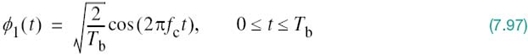
Then, we may respectively express the transmitted signals s₁(t) and s₂(t) in terms of ϕ₁(t) as

A binary PSK system is, therefore, characterized by having a signal space that is one-dimensional (i.e., N = 1), with a signal constellation consisting of two message points (i.e., M = 2). The respective coordinates of the two message points are

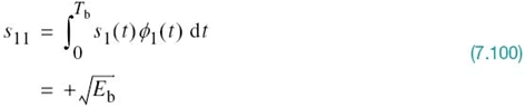
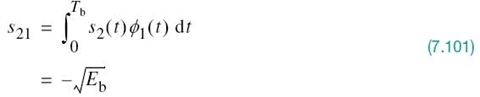
In words, the message point corresponding to s₁(t) is located at and the message point corresponding to s₂(t) is located at . Figure 7.13a displays the signal-space diagram for binary PSK and Figure 7.13b shows example waveforms of antipodal signals representing s₁(t) and s₂(t). Note that the binary constellation of Figure 7.13 has minimum average energy.

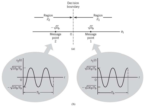
Figure 7.13 (a) Signal-space diagram for coherent binary PSK system. (b) The waveforms depicting the transmitted signals s₁(t) and s₂(t), assuming n_c = 2.

Generation of a binary PSK signal follows readily from (7.97) to (7.99). Specifically, as shown in the block diagram of Figure 7.14a, the generator (transmitter) consists of two components:

1.  Polar NRZ-level encoder, which represents symbols 1 and 0 of the incoming binary sequence by amplitude levels and respectively.

2.  Product modulator, which multiplies the output of the polar NRZ encoder by the basis function ϕ₁(t); in effect, the sinusoidal ϕ₁(t) acts as the “carrier” of the binary PSK signal.

Accordingly, binary PSK may be viewed as a special form of DSB-SC modulation that was studied in Section 2.14.

Error Probability of Binary PSK Using Coherent Detection

To make an optimum decision on the received signal x(t) in favor of symbol 1 or symbol 0 (i.e., estimate the original binary sequence at the transmitter input), we assume that the receiver has access to a locally generated replica of the basis function ϕ₁(t). In other words, the receiver is synchronized with the transmitter, as shown in the block diagram of Figure 7.14b. We may identify two basic components in the binary PSK receiver:

1.  Correlator, which correlates the received signal x(t) with the basis function ϕ₁(t) on a bit-by-bit basis.

2.  Decision device, which compares the correlator output against a zero-threshold, assuming that binary symbols 1 and 0 are equiprobable. If the threshold is exceeded, a decision is made in favor of symbol 1; if not, the decision is made in favor of symbol 0. Equality of the correlator with the zero-threshold is decided by the toss of a fair coin (i.e., in a random manner).

With coherent detection in place, we may apply the decision rule of (7.54). Specifically, we partition the signal space of Figure 7.13 into two regions:

• the set of points closest to message point 1 at ; and
• the set of points closest to message point 2 at.

This is accomplished by constructing the midpoint of the line joining these two message points and then marking off the appropriate decision regions. In Figure 7.13, these two decision regions are marked Z₁ and Z₂, according to the message point around which they are constructed.

The decision rule is now simply to decide that signal s₁(t) (i.e., binary symbol 1) was transmitted if the received signal point falls in region Z₁ and to decide that signal s₂(t) (i.e., binary symbol 0) was transmitted if the received signal point falls in region Z₂. Two kinds of erroneous decisions may, however, be made:

1.  Error of the first kind. Signal s₂(t) is transmitted but the noise is such that the received signal point falls inside region Z₁; so the receiver decides in favor of signal s₁(t).

2.  Error of the second kind. Signal s₁(t) is transmitted but the noise is such that the received signal point falls inside region Z₂; so the receiver decides in favor of signal s₂(t).

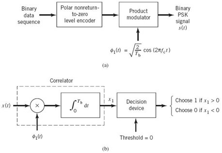
Figure 7.14 Block diagrams for (a) binary PSK transmitter and (b) coherent binary PSK receiver.

To calculate the probability of making an error of the first kind, we note from Figure 7.13a that the decision region associated with symbol 1 or signal s₁(t) is described by

where the observable element x₁ is related to the received signal x(t) by

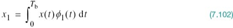
The conditional probability density function of random variable X₁, given that symbol 0 (i.e., signal s₂(t)) was transmitted, is defined by

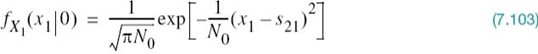
Using (7.101) in this equation yields

The conditional probability of the receiver deciding in favor of symbol 1, given that symbol 0 was transmitted, is therefore

Putting

and changing the variable of integration from x₁ to z, we may compactly rewrite (7.105) in terms of the Q-function:

Using the formula of (3.68) in Chapter 3 for the Q-function in (7.107) we get

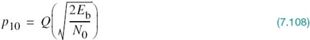
Consider next an error of the second kind. We note that the signal space of Figure 7.13a is symmetric with respect to the origin. It follows, therefore, that p₀₁, the conditional probability of the receiver deciding in favor of symbol 0, given that symbol 1 was transmitted, also has the same value as in (7.108).

Thus, averaging the conditional error probabilities p₁₀ and p₀₁, we find that the average probability of symbol error or, equivalently, the BER for binary PSK using coherent detection and assuming equiprobable symbols is given by

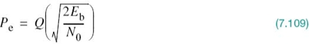
As we increase the transmitted signal energy per bit E_b for a specified noise spectral density N₀/2, the message points corresponding to symbols 1 and 0 move further apart and the average probability of error P_e is correspondingly reduced in accordance with (7.109), which is intuitively satisfying.

Power Spectra of Binary PSK Signals

Examining (7.97) and (7.98), we see that a binary PSK wave is an example of DSB-SC modulation that was discussed in Section 2.14. More specifically, it consists of an in-phase component only. Let g(t) denote the underlying pulse-shaping function defined by

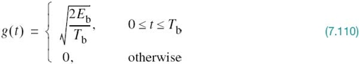
Depending on whether the transmitter input is binary symbol 1 or 0, the corresponding transmitter output is +g(t) or –g(t), respectively. It is assumed that the incoming binary sequence is random, with symbols 1 and 0 being equally likely and the symbols transmitted during the different time slots being statistically independent.

In Example 6 of Chapter 4, it was shown that the power spectral density of a random binary wave so described is equal to the energy spectral density of the symbol shaping function divided by the symbol duration. The energy spectral density of a Fourier-transformable signal g(t) is defined as the squared magnitude of the signal’s Fourier transform. For the binary PSK signal at hand, the baseband power spectral density is, therefore, defined by

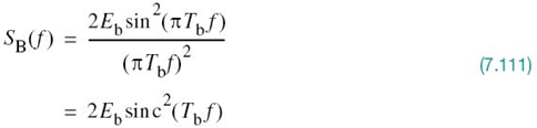
Examining (7.111), we may make the following observations on binary PSK:

1.  The power spectral density S_B(f) is symmetric about the vertical axis, as expected.

2.  S_B(f) goes through zero at multiples of the bit rate; that is, f = ±1/T_b, ±2/T_b,…

3.  With sin²(πT_bf) limited to a maximum value of unity, S_B(f) falls off as the inverse square of the frequency, f.

These three observations are all embodied in the plot of S_B(f) versus f, presented in Figure 7.15.

Figure 7.15 also includes a plot of the baseband power spectral density of a binary frequency-shift keying (FSK) signal, details of which are presented in Section 7.8. Comparison of these two spectra is deferred to that section.

Quadriphase-Shift Keying

The provision of reliable performance, exemplified by a very low probability of error, is one important goal in the design of a digital communication system. Another important goal is the efficient utilization of channel bandwidth. In this subsection we study a bandwidth-conserving modulation scheme known as quadriphase-shift keying (QPSK), using coherent detection.

As with binary PSK, information about the message symbols in QPSK is contained in the carrier phase. In particular, the phase of the carrier takes on one of four equally spaced values, such as π/4, 3π/4, 5π/4, and 7π/4. For this set of values, we may define the transmitted signal as

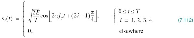
where E is the transmitted signal energy per symbol and T is the symbol duration. The carrier frequency f_c equals n_c/T for some fixed integer n_c. Each possible value of the phase corresponds to a unique dibit (i.e., pair of bits). Thus, for example, we may choose the foregoing set of phase values to represent the Gray-encoded set of dibits, 10, 00, 01, and 11, where only a single bit is changed from one dibit to the next.

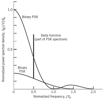
Figure 7.15 Power spectra of binary PSK and FSK signals.

Signal-Space Diagram of QPSK Signals

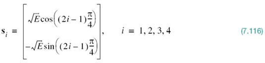
Using a well-known trigonometric identity, we may expand (7.112) to redefine the transmitted signal in the canonical form:

where i = 1, 2, 3, 4. Based on this representation, we make two observations:

1.  There are two orthonormal basis functions, defined by a pair of quadrature carriers:

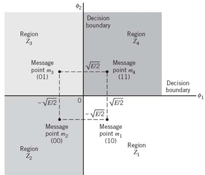
Figure 7.16 Signal-space diagram of QPSK system.

Table 7.2 Signal-space characterization of QPSK

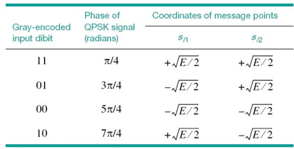
2.  There are four message points, defined by the two-dimensional signal vector

Elements of the signal vectors, namely s_i1 and s_i2, have their values summarized in Table 7.2; the first two columns give the associated dibit and phase of the QPSK signal.

Accordingly, a QPSK signal has a two-dimensional signal constellation (i.e., N = 2) and four message points (i.e., M = 4) whose phase angles increase in a counterclockwise direction, as illustrated in Figure 7.16. As with binary PSK, the QPSK signal has minimum average energy.

EXAMPLE 6  QPSK Waveforms

Figure 7.17 illustrates the sequences and waveforms involved in the generation of a QPSK signal. The input binary sequence 01101000 is shown in Figure 7.17a. This sequence is divided into two other sequences, consisting of odd- and even-numbered bits of the input sequence. These two sequences are shown in the top lines of Figure 7.17b and c. The waveforms representing the two components of the QPSK signal, namely s_i1ϕ₁(t) and s_i2ϕ₂(t) are also shown in Figure 7.17b and c, respectively. These two waveforms may individually be viewed as examples of a binary PSK signal. Adding them, we get the QPSK waveform shown in Figure 7.17d.

To define the decision rule for the coherent detection of the transmitted data sequence, we partition the signal space into four regions, in accordance with Table 7.2. The individual regions are defined by the set of symbols closest to the message point represented by message vectors s₁, s₂, s₃, and s₄. This is readily accomplished by constructing the perpendicular bisectors of the square formed by joining the four message points and then marking off the appropriate regions. We thus find that the decision regions are quadrants whose vertices coincide with the origin. These regions are marked Z₁,Z₂, Z₃, and Z₄ in Figure 7.17, according to the message point around which they are constructed.

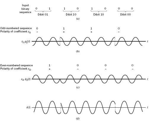
Figure 7.17 (a) Input binary sequence. (b) Odd-numbered dibits of input sequence and associated binary PSK signal. (c) Even-numbered dibits of input sequence and associated binary PSK signal.(d) QPSK waveform defined as s(t) = s_i1 ϕ₁ (t) + s_i2ϕ₂ (t).

Generation and Coherent Detection of QPSK Signals

Expanding on the binary PSK transmitter of Figure 7.14a, we may build on (7.113) to (7.115) to construct the QPSK transmitter shown in Figure 7.18a. A distinguishing feature of the QPSK transmitter is the block labeled demultiplexer. The function of the demultiplexer is to divide the binary wave produced by the polar NRZ-level encoder into two separate binary waves, one of which represents the odd-numbered dibits in the incoming binary sequence and the other represents the even-numbered dibits. Accordingly, we may make the following statement:

The QPSK transmitter may be viewed as two binary PSK generators that work in parallel, each at a bit rate equal to one-half the bit rate of the original binary sequence at the QPSK transmitter input.

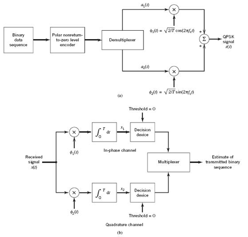
Figure 7.18 Block diagram of (a) QPSK transmitter and (b) coherent QPSK receiver.

Expanding on the binary PSK receiver of Figure 7.14b, we find that the QPSK receiver is structured in the form of an in-phase path and a quadrature path, working in parallel as depicted in Figure 7.18b. The functional composition of the QPSK receiver is as follows:

1.  Pair of correlators, which have a common input x(t). The two correlators are supplied with a pair of locally generated orthonormal basis functions ϕ₁(t) and ϕ₂(t), which means that the receiver is synchronized with the transmitter. The correlator outputs, produced in response to the received signal x(t), are denoted by x₁ and x₂, respectively.

2.  Pair of decision devices, which act on the correlator outputs x₁ and x₂ by comparing each one with a zero-threshold; here, it is assumed that the symbols 1 and 0 in the original binary stream at the transmitter input are equally likely. If x₁> 0, a decision is made in favor of symbol 1 for the in-phase channel output; on the other hand, if x₁ < 0, then a decision is made in favor of symbol 0. Similar binary decisions are made for the quadrature channel.

3.  Multiplexer, the function of which is to combine the two binary sequences produced by the pair of decision devices. The resulting binary sequence so produced provides an estimate of the original binary stream at the transmitter input.

Error Probability of QPSK

In a QPSK system operating on an AWGN channel, the received signal x(t) is defined by

where w(t) is the sample function of a white Gaussian noise process of zero mean and power spectral density N₀/2.

Referring to Figure 7.18a, we see that the two correlator outputs, x₁ and x₂, are respectively defined as follows:

and

Thus, the observable elements x₁ and x₂ are sample values of independent Gaussian random variables with mean values equal to and , respectively, and with a common variance equal to N₀/2.

The decision rule is now simply to say that s₁(t) was transmitted if the received signal point associated with the observation vector x falls inside region Z₁; say that s₂(t) was transmitted if the received signal point falls inside region Z₂, and so on for the other two regions Z₃ and Z₄. An erroneous decision will be made if, for example, signal s₄(t) is transmitted but the noise w(t) is such that the received signal point falls outside region Z₄.

To calculate the average probability of symbol error, recall that a QPSK receiver is in fact equivalent to two binary PSK receivers working in parallel and using two carriers that are in phase quadrature. The in-phase channel x₁ and the quadrature channel output x₂ (i.e., the two elements of the observation vector x) may be viewed as the individual outputs of two binary PSK receivers. Thus, according to (7.118) and (7.119), these two binary PSK receivers are characterized as follows:

• signal energy per bit equal to E/2, and
• noise spectral density equal to N₀/2.

Hence, using (7.109) for the average probability of bit error of a coherent binary PSK receiver, we may express the average probability of bit error in the in-phase and quadrature paths of the coherent QPSK receiver as

where E is written in place of 2E_b. Another important point to note is that the bit errors in the in-phase and quadrature paths of the QPSK receiver are statistically independent. The decision device in the in-phase path accounts for one of the two bits constituting a symbol (dibit) of the QPSK signal, and the decision device in the quadrature path takes care of the other dibit. Accordingly, the average probability of a correct detection resulting from the combined action of the two channels (paths) working together is

The average probability of symbol error for QPSK is therefore

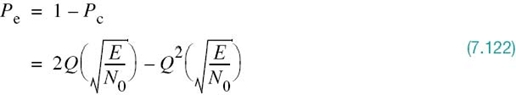
In the region where (E/N₀) >> 1, we may ignore the quadratic term on the right-hand side of (7.122), so the average probability of symbol error for the QPSK receiver is approximated as

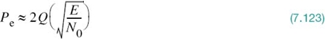
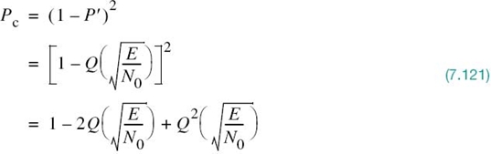
Equation (7.123) may also be derived in another insightful way, using the signal-space diagram of Figure 7.16. Since the four message points of this diagram are circularly symmetric with respect to the origin, we may apply the approximate formula of (7.85) based on the union bound. Consider, for example, message point m₁ (corresponding to dibit 10) chosen as the transmitted message point. The message points m₂ and m₄ (corresponding to dibits 00 and 11) are the closest to m₁. From Figure 7.16 we readily find that m₁ is equidistant from m₂ and m₄ in a Euclidean sense, as shown by

Assuming that E/N₀ is large enough to ignore the contribution of the most distant message point m₃ (corresponding to dibit 01) relative to m₁, we find that the use of (7.85) with the equality sign yields an approximate expression for P_e that is the same as that of (7.123). Note that in mistaking either m₂ or m₄ for m₁, a single bit error is made; on the other hand, in mistaking m₃ for m₁, two bit errors are made. For a high enough E/N₀, the likelihood of both bits of a symbol being in error is much less than a single bit, which is a further justification for ignoring m₃ in calculating P_e when m₁ is sent.

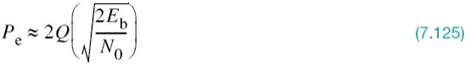
In a QPSK system, we note that since there are two bits per symbol, the transmitted signal energy per symbol is twice the signal energy per bit, as shown by

Thus, expressing the average probability of symbol error in terms of the ratio E_b/N₀, we may write

With Gray encoding used for the incoming symbols, we find from (7.120) and (7.124) that the BER of QPSK is exactly

We may, therefore, state that a QPSK system achieves the same average probability of bit error as a binary PSK system for the same bit rate and the same E_b/N₀, but uses only half the channel bandwidth. Stated in another way:

For the same E_b/N₀ and, therefore, the same average probability of bit error, a QPSK system transmits information at twice the bit rate of a binary PSK system for the same channel bandwidth.

For a prescribed performance, QPSK uses channel bandwidth better than binary PSK, which explains the preferred use of QPSK over binary PSK in practice.

Earlier we stated that the binary PSK may be viewed as a special case of DSB-SC modulation. In a corresponding way, we may view the QPSK as a special case of the quadrature amplitude modulation (QAM) in analog modulation theory.

Power Spectra of QPSK Signals

Assume that the binary wave at the modulator input is random with symbols 1 and 0 being equally likely, and with the symbols transmitted during adjacent time slots being statistically independent. We then make the following observations pertaining to the in-phase and quadrature components of a QPSK signal:

1.  Depending on the dibit sent during the signaling interval –T_b ≤ t ≤ T_b, the in-phase component equals +g(t) or –g(t), and similarly for the quadrature component. The g(t) denotes the symbol-shaping function defined by

Hence, the in-phase and quadrature components have a common power spectral density, namely, E sinc²(Tf).

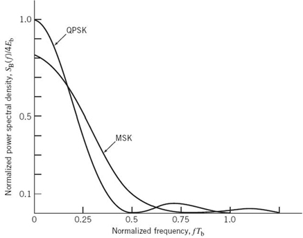
Figure 7.19 Power spectra of QPSK and MSK signals.

2. The in-phase and quadrature components are statistically independent. Accordingly, the baseband power spectral density of the QPSK signal equals the sum of the individual power spectral densities of the in-phase and quadrature components, so we may write

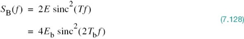
Figure 7.19 plots S_B(f), normalized with respect to 4E_b, versus the normalized frequency T_bf. This figure also includes a plot of the baseband power spectral density of a certain form of binary FSK called minimum shift keying, the evaluation of which is presented in Section 7.8. Comparison of these two spectra is deferred to that section.

Offset QPSK

For a variation of the QPSK, consider the signal-space diagram of Figure 7.20a, that embodies all the possible phase transitions that can arise in the generation of a QPSK signal. More specifically, examining the QPSK waveform illustrated in Figure 7.17 for Example 6, we may make three observations:

1.  The carrier phase changes by ±180° whenever both the in-phase and quadrature components of the QPSK signal change sign. An example of this situation is illustrated in Figure 7.17 when the input binary sequence switches from dibit 01 to dibit 10.

2.  The carrier phase changes by ±90° whenever the in-phase or quadrature component changes sign. An example of this second situation is illustrated in Figure 7.17 when the input binary sequence switches from dibit 10 to dibit 00, during which the in-phase component changes sign, whereas the quadrature component is unchanged.

3.  The carrier phase is unchanged when neither the in-phase component nor the quadrature component changes sign. This last situation is illustrated in Figure 7.17 when dibit 10 is transmitted in two successive symbol intervals.

Situation 1 and, to a much lesser extent, situation 2 can be of a particular concern when the QPSK signal is filtered during the course of transmission, prior to detection. Specifically, the 180° and 90° shifts in carrier phase can result in changes in the carrier amplitude (i.e., envelope of the QPSK signal) during the course of transmission over the channel, thereby causing additional symbol errors on detection at the receiver.

To mitigate this shortcoming of QPSK, we need to reduce the extent of its amplitude fluctuations. To this end, we may use offset QPSK.⁴ In this variant of QPSK, the bit stream responsible for generating the quadrature component is delayed (i.e., offset) by half a symbol interval with respect to the bit stream responsible for generating the in-phase component. Specifically, the two basis functions of offset QPSK are defined by

and

The ϕ₁(t) of (7.129) is exactly the same as that of (7.114) for QPSK, but the ϕ₂(t) of (7.130) is different from that of (7.115) for QPSK. Accordingly, unlike QPSK, the phase transitions likely to occur in offset QPSK are confined to ±90°, as indicated in the signal-space diagram of Figure 7.20b,. However, ±90° phase transitions in offset QPSK occur twice as frequently but with half the intensity encountered in QPSK. Since, in addition to ±90° phase transitions, ±180° phase transitions also occur in QPSK, we find that amplitude fluctuations in offset QPSK due to filtering have a smaller amplitude than in the case of QPSK.

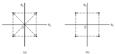
Figure 7.20 Possible paths for switching between the message points in (a) QPSK and (b) offset QPSK.

Despite the delay T/2 applied to the basis function ϕ₂(t) in (7.130) compared with that in (7.115) for QPSK, the offset QPSK has exactly the same probability of symbol error in an AWGN channel as QPSK. The equivalence in noise performance between these PSK schemes assumes the use of coherent detection at the receiver. The reason for the equivalence is that the statistical independence of the in-phase and quadrature components applies to both QPSK and offset QPSK. We may, therefore, say that Equation (7.123) for the average probability of symbol error applies equally well to the offset QPSK.

M-ary PSK

QPSK is a special case of the generic form of PSK commonly referred to as M-ary PSK, where the phase of the carrier takes on one of M possible values: θ_i = 2(i – 1)π/M, where i = 1,2,…,M. Accordingly, during each signaling interval of duration T, one of the M possible signals

is sent, where E is the signal energy per symbol. The carrier frequency f_c = n_c/T for some fixed integer n_c.

Each s_i(t) may be expanded in terms of the same two basis functions ϕ₁(t) and ϕ₂(t); the signal constellation of M-ary PSK is, therefore, two-dimensional. The M message points are equally spaced on a circle of radius and center at the origin, as illustrated in Figure 7.21a, for the case of octaphase-shift-keying (i.e., M = 8).

From Figure 7.21a, we see that the signal-space diagram is circularly symmetric. We may, therefore, apply (7.85), based on the union bound, to develop an approximate formula for the average probability of symbol error for M-ary PSK. Suppose that the transmitted signal corresponds to the message point m₁, whose coordinates along the ϕ₁- and ϕ₂-axes are + and 0, respectively. Suppose that the ratio E/N₀ is large enough to consider the nearest two message points, one on either side of m₁, as potential candidates for being mistaken for m₁ due to channel noise. This is illustrated in Figure 7.21b, for the case of M = 8. TheEuclidean distance for each of these two points from m₁ is (for M = 8)

Hence, the use of (7.85) yields the average probability of symbol error for coherent M-ary PSK as

where it is assumed that M ≥ 4. The approximation becomes extremely tight for fixed M, as E/N₀ is increased. For M = 4, (7.132) reduces to the same form given in (7.123) for QPSK.

Power Spectra of M-ary PSK Signals

The symbol duration of M-ary PSK is defined by

where T_b is the bit duration. Proceeding in a manner similar to that described for a QPSK signal, we may show that the baseband power spectral density of an M-ary PSK signal is given by

Figure 7.22 is a plot of the normalized power spectral density S_B(f)/2E_b versus the normalized frequency T_bf for three different values of M, namely M = 2, 4, 8. Equation (7.134) includes (7.111) for M = 2 and (7.128) for M = 4 as two special cases.

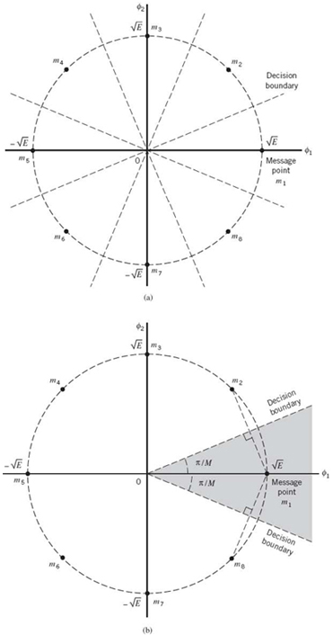
Figure 7.21 (a) Signal-space diagram for octaphase-shift keying (i.e., M = 8). The decision boundaries are shown as dashed lines. (b) Signal-space diagram illustrating the application of the union bound for octaphase-shift keying.

The baseband power spectra of M-ary PSK signals plotted in Figure 7.22, possess a main lobe bounded by well-defined spectral nulls (i.e., frequencies at which the power spectral density is zero). In light of the discussion on the bandwidth of signals presented in Chapter 2, we may use the main lobe as a basis for bandwidth assessment. Accordingly, invoking the notion of null-to-null bandwidth, we may say that the spectral width of the main lobe provides a simple, yet informative, measure for the bandwidth of M-ary PSK signals. Most importantly, a large fraction of the average signal power is contained inside the main lobe. On this basis, we may define the channel bandwidth required to pass M-ary PSK signals through an analog channel as

where T is the symbol duration. But the symbol duration T is related to the bit duration T_b by (7.133). Moreover, the bit rate R_b = 1/T_b. Hence, we may redefine the channel bandwidth of (7.135) in terms of the bit rate as

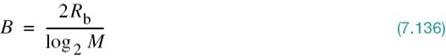
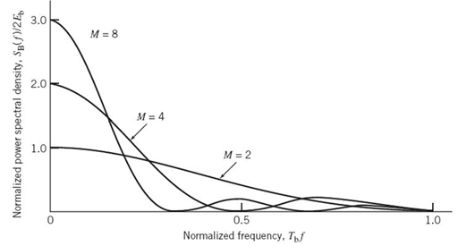
Figure 7.22 Power spectra of M-ary PSK signals for M = 2, 4, 8.

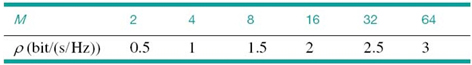
Table 7.3 Bandwidth efficiency of M-ary PSK signals

Based on this formula, the bandwidth efficiency of M-ary PSK signals is given by

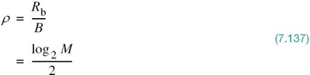
Table 7.3 gives the values of ρ calculated from (7.137) for varying M. In light of (7.132) and Table 7.3, we now make the statement:

As the number of states in M-ary PSK is increased, the bandwidth efficiency is improved at the expense of error performance.

However, note that if we are to ensure that there is no degradation in error performance, we have to increase E_b/N₀ to compensate for the increase in M.

7.7    M-ary Quadrature Amplitude Modulation

In an M-ary PSK system, the in-phase and quadrature components of the modulated signal are interrelated in such a way that the envelope is constrained to remain constant. This constraint manifests itself in a circular constellation for the message points, as illustrated in Figure 7.21a,. However, if this constraint is removed so as to permit the in-phase and quadrature components to be independent, we get a new modulation scheme called M-ary QAM. The QAM is a hybrid form of modulation, in that the carrier experiences amplitude as well as phase-modulation.

In M-ary PAM, the signal-space diagram is one-dimensional. M-ary QAM is a two-dimensional generalization of M-ary PAM, in that its formulation involves two orthogonal passband basis functions:

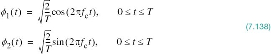
Let d_min denote the minimum distance between any two message points in the QAM constellation. Then, the projections of the i th message point on the ϕ₁- and ϕ₂-axes are respectively defined by a_i d_min/2 and b_i d_min/2, where i = 1,2,…,M. With the separation between two message points in the signal-space diagram being proportional to the square root of energy, we may therefore set

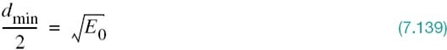
where E₀ is the energy of the message signal with the lowest amplitude. The transmitted M-ary QAM signal for symbol k can now be defined in terms of E₀:

The signal s_k(t) involves two phase-quadrature carriers, each one of which is modulated by a set of discrete amplitudes; hence the terminology “quadrature amplitude modulation.”

In M-ary QAM, the constellation of message points depends on the number of possible symbols, M. In what follows, we consider the case of square constellations, for which the number of bits per symbol is even.

QAM Square Constellations

With an even number of bits per symbol, we write

Under this condition, an M-ary QAM square constellation can always be viewed as the Cartesian product of a one-dimensional L-ary PAM constellation with itself. By definition, the Cartesian product of two sets of coordinates (representing a pair of one-dimensional constellations) is made up of the set of all possible ordered pairs of coordinates with the first coordinate in each such pair being taken from the first set involved in the product and the second coordinate taken from the second set in the product.

Thus, the ordered pairs of coordinates naturally form a square matrix, as shown by

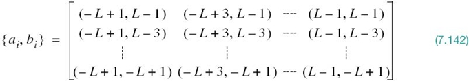
To calculate the probability of symbol error for this M-ary QAM, we exploit the following property:

A QAM square constellation can be factored into the product of the corresponding L-ary PAM constellation with itself.

To exploit this statement, we may proceed in one of two ways:

Approach 1: We start with a signal constellation of the M-ary PAM for a prescribed M, and then build on it to construct the corresponding signal constellation of the M-ary QAM.

Approach 2: We start with a signal constellation of the M-ary QAM, and then use it to construct the corresponding orthogonal M-ary PAMS.

In the example to follow, we present a systematic procedure based on Approach 1.

EXAMPLE 7  M-ary QAM for M = 4

In Figure 7.23, we have constructed two signal constellations for the 4-ary PAM, one vertically oriented along the ϕ₁-axis in part a of the figure, and the other horizontally oriented along the ϕ₂-axis in part b of the figure. These two parts are spatially orthogonal to each other, accounting for the two-dimensional structure of the M-ary QAM. In developing this structure, the following points should be born in mind:

• The same binary sequence is used for both 4-ary PAM constellations.
• The Gray encoding rule is applied, which means that as we move from one codeword to an adjacent one, only a single bit is changed.
• In constructing the 4-ary QAM constellation, we move from one quadrant to the next in a counterclockwise direction.

With four quadrants constituting the 4-ary QAM, we proceed in four stages as follows:

Stage 1: First-quadrant constellation. Referring to Figure 7.23,, we use the codewords along the positive parts of the ϕ₂ and ϕ₁-axes, respectively, to write

Stage 2: Second-quadrant constellation. Following the same procedure as in Stage 1, we write

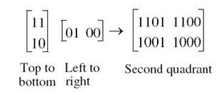
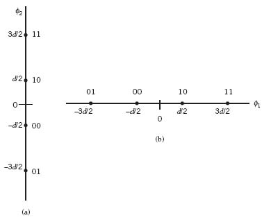
Figure 7.23 The two orthogonal constellations of the 4-ary PAM. (a) Vertically oriented constellation. (b) Horizontally oriented constellation. As mentioned in the text, we move top-down along the ϕ₂-axis and from left to right along the ϕ₁-axis.

Stage 3: Third-quadrant constellation. Again, following the same procedure as before, we next write

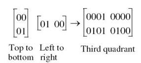
Stage 4: Fourth-quadrant constellation. Finally, we write

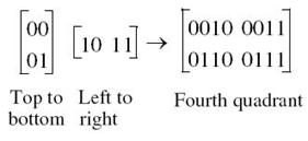
The final step is to piece together these four constituent 4-ary PAM constellations to construct the 4-ary QAM constellations as described in Figure 7.24,. The important point to note here is that all the codewords in Figure 7.24, obey the Gray encoding rule, not only within each quadrant but also as we move from one quadrant to the next.

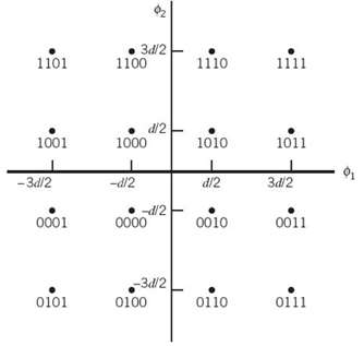
Figure 7.24 (a) Signal-space diagram of M-ary QAM for M = 16; the message points in each quadrant are identified with Gray-encoded quadbits.

Average Probability of Error

In light of the equivalence established between the M-ary QAM and M-ary PAM, we may formulate the average probability of error of the M-ary QAM by proceeding as follows:

1.  The probability of correct detection for M-ary QAM is written as

where p'_e is the probability of symbol error for the L-ary PAM.

2.  With the probability of symbol error p'_e is itself defined by

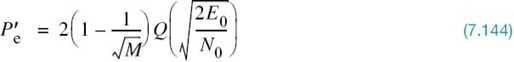
3.  The probability of symbol error for M-ary QAM is given by

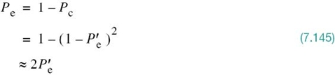
where it is assumed that is p'_e small enough compared with unity to justify ignoring the quadratic term.

Hence, using (7.143) and (7.144) in (7.145), we find that the probability of symbol error for M-ary QAM is approximately given by

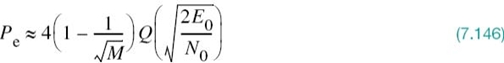
The transmitted energy in M-ary QAM is variable, in that its instantaneous value naturally depends on the particular symbol transmitted. Therefore, it is more logical to express P_e in terms of the average value of the transmitted energy rather than E₀. Assuming that the L amplitude levels of the in-phase or quadrature component of the M-ary QAM signal are equally likely, we have

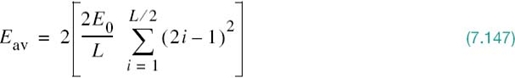
where the overall scaling factor 2 accounts for the equal contributions made by the in-phase and quadrature components. The limits of the summation and the scaling factor 2 inside the large parentheses account for the symmetric nature of the pertinent amplitude levels around zero. Summing the series in (7.147), we get

Accordingly, we may rewrite (7.146) in terms of E_av as

which is the desired result.

The case of M = 4 is of special interest. The signal constellation for this particular value of M is the same as that for QPSK. Indeed, putting M = 4 in (7.150) and noting that, for this special case, E_av equals E, where E is the energy per symbol, we find that the resulting formula for the probability of symbol error becomes identical to that in (7.123) for QPSK; and so it should.

7.8 Frequency-Shift Keying Techniques Using Coherent Detection

M-ary PSK and M-ary QAM share a common property: both of them are examples of linear modulation. In this section, we study a nonlinear method of modulation known as FSK using coherent detection. We begin the study by considering the simple case of binary FSK, for which M = 2.

Binary FSK

In binary FSK, symbols 1 and 0 are distinguished from each other by transmitting one of two sinusoidal waves that differ in frequency by a fixed amount. A typical pair of sinusoidal waves is described by

where i = 1, 2 and E_b is the transmitted signal energy per bit; the transmitted frequency is set at

Symbol 1 is represented by s₁(t) and symbol 0 by s₂(t). The FSK signal described here is known as Sunde’s FSK. It is a continuous-phase signal, in the sense that phase continuity is always maintained, including the inter-bit switching times.

From (7.151) and (7.152), we observe directly that the signals s₁(t) and s₂(t) are orthogonal, but not normalized to have unit energy. The most useful form for the set of orthonormal basis functions is described by

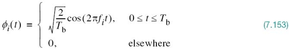
where i = 1, 2. Correspondingly, the coefficient s_ij for where i = 1, 2 and j = 1, 2 is defined by

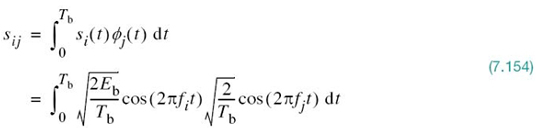
Carrying out the integration in (7.154), the formula for s_ij simplifies to

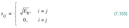
Thus, unlike binary PSK, binary FSK is characterized by having a signal-space diagram that is two-dimensional (i.e., N = 2) with two message points (i.e., M = 2), as shown in Figure 7.25. The two message points are defined by the vectors

and

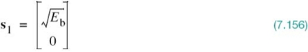
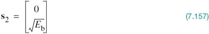
The Euclidean distance is equal to . Figure 7.25 also includes a couple of waveforms representative of signals s₁(t) and s₂(t).

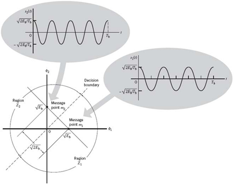
Figure 7.25 Signal-space diagram for binary FSK system. The diagram also includes example waveforms of the two modulated signals s₁(t) and s₂(t).

Generation and Coherent Detection of Binary FSK Signals

The block diagram of Figure 7.26a describes a scheme for generating the binary FSK signal; it consists of two components:

1.  On–off level encoder, the output of which is a constant amplitude of in response to input symbol 1 and zero in response to input symbol 0.

2.  Pair of oscillators, whose frequencies f₁ and f₂ differ by an integer multiple of the bit rate 1/T_b in accordance with (7.152). The lower oscillator with frequency f₂ is preceded by an inverter. When in a signaling interval, the input symbol is 1, the upper oscillator with frequency f₁ is switched on and signal s₁(t) is transmitted, while the lower oscillator is switched off. On the other hand, when the input symbol is 0, the upper oscillator is switched off, while the lower oscillator is switched on and signal s₂(t) with frequency f₂ is transmitted. With phase continuity as a requirement, the two oscillators are synchronized with each other. Alternatively, we may use a voltage-controlled oscillator, in which case phase continuity is automatically satisfied.

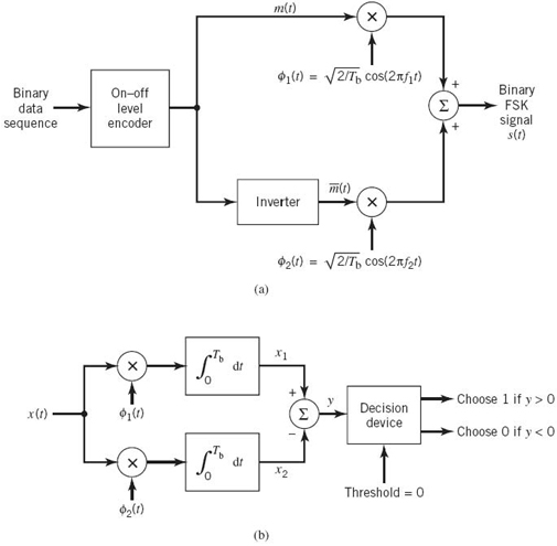
Figure 7.26 Block diagram for (a) binary FSK transmitter and (b) coherent binary FSK receiver.

To coherently detect the original binary sequence given the noisy received signal x(t), we may use the receiver shown in Figure 7.26b. It consists of two correlators with a common input, which are supplied with locally generated coherent reference signals ϕ₁(t) and ϕ₂(t). The correlator outputs are then subtracted, one from the other; the resulting difference y is then compared with a threshold of zero. If y > 0, the receiver decides in favor of 1. On the other hand, if y < 0, it decides in favor of 0. If y is exactly zero, the receiver makes a random guess (i.e., flip of a fair coin) in favor of 1 or 0.

Error Probability of Binary FSK

The observation vector x has two elements x₁ and x₂ that are defined by, respectively,

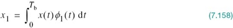
and

where x(t) is the received signal, whose form depends on which symbol was transmitted. Given that symbol 1 was transmitted, x(t) equals s₁(t) + w(t), where w(t) is the sample function of a white Gaussian noise process of zero mean and power spectral density N₀/2. If, on the other hand, symbol 0 was transmitted, x(t) equals s₂(t) + w(t).

Now, applying the decision rule of (7.57) assuming the use of coherent detection at the receiver, we find that the observation space is partitioned into two decision regions, labeled Z₁ and Z₂ in Figure 7.25. The decision boundary, separating region Z₁ from region Z₂, is the perpendicular bisector of the line joining the two message points. The receiver decides in favor of symbol 1 if the received signal point represented by the observation vector x falls inside region Z₁. This occurs when x₁ < x₂. If, on the other hand, we have x₁ > x₂, the received signal point falls inside region Z₂ and the receiver decides in favor of symbol 0. On the decision boundary, we have x₁ = x₂, in which case the receiver makes a random guess in favor of symbol 1 or 0.

To proceed further, we define a new Gaussian random variable Y whose sample value y is equal to the difference between x₁ and x₂; that is,

The mean value of the random variable Y depends on which binary symbol was transmitted. Given that symbol 1 was sent, the Gaussian random variables X₁ and X₂, whose sample values are denoted by x₁ and x₂, have mean values equal to and zero, respectively. Correspondingly, the conditional mean of the random variable Y given that symbol 1 was sent is

On the other hand, given that symbol 0 was sent, the random variables X₁ and X₂ have mean values equal to zero and , respectively. Correspondingly, the conditional mean of the random variable Y given that symbol 0 was sent is

The variance of the random variable Y is independent of which binary symbol was sent. Since the random variables X₁ and X₂ are statistically independent, each with a variance equal to N₀/2, it follows that

Suppose we know that symbol 0 was sent. The conditional probability density function of the random variable Y is then given by

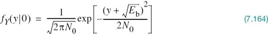
Since the condition x₁ > x₂ or, equivalently, y > 0 corresponds to the receiver making a decision in favor of symbol 1, we deduce that the conditional probability of error given that symbol 0 was sent is

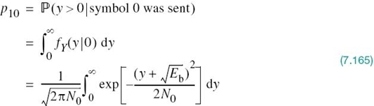
To put the integral in (7.165) in a standard form involving the Q-function, we set

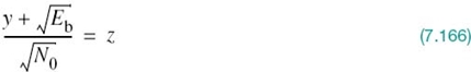
Then, changing the variable of integration from y to z, we may rewrite (7.165) as

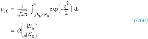
Similarly, we may show the p₀₁, the conditional probability of error given that symbol 1 was sent, has the same value as in (7.167). Accordingly, averaging p₁₀ and p₀₁ and assuming equiprobable symbols, we find that the average probability of bit error or, equivalently, the BER for binary FSK using coherent detection is

Comparing (7.108) and (7.168), we see that for a binary FSK receiver to maintain the same BER as in a binary PSK receiver, the bit energy-to-noise density ratio, E_b/N₀, has to be doubled. This result is in perfect accord with the signal-space diagrams of Figures 7.13 and 7.25, where we see that in a binary PSK system the Euclidean distance between the two message points is equal to , whereas in a binary FSK system the corresponding distance is . For a prescribed E_b, the minimum distance d_min in binary PSK is, therefore, times that in binary FSK. Recall from (7.89) that the probability of error decreases exponentially as d²_min; hence the difference between (7.108) and (7.168).

Power Spectra of Binary FSK Signals

Consider the case of Sunde's FSK, for which the two transmitted frequencies f₁ and f₂ differ by an amount equal to the bit rate 1/T_b, and their arithmetic mean equals the nominal carrier frequency f_c; as mentioned previously, phase continuity is always maintained, including inter-bit switching times. We may express this special binary FSK signal as a frequency-modulated signal, defined by

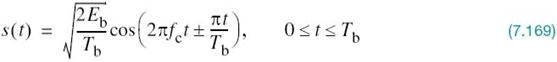
Using a well-known trigonometric identity, we may reformulate s(t) in the expanded form

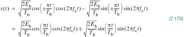
In the last line of (7.170), the plus sign corresponds to transmitting symbol 0 and the minus sign corresponds to transmitting symbol 1. As before, we assume that the symbols 1 and 0 in the binary sequence applied to the modulator input are equally likely, and that the symbols transmitted in adjacent time slots are statistically independent. Then, based on the representation of (7.170), we may make two observations pertaining to the in-phase and quadrature components of a binary FSK signal with continuous phase:

1. The in-phase component is completely independent of the input binary wave. It equals for all time t. The power spectral density of this component, therefore, consists of two delta functions at t = ± 1/2T_b and weighted by the factor E_b/2T_b, and occurring at f = ± 1/2T_b.

2.  The quadrature component is directly related to the input binary sequence. During the signaling interval 0 ≤ t ≤ T_b, it equals –g(t) when we have symbol 1 and +g(t) when we have symbol 0, with g(t) denoting a symbol-shaping function defined by

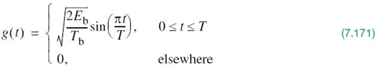
The energy spectral density of g(t) is defined by

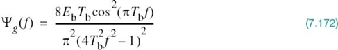
The power spectral density of the quadrature component equals. It is also apparent that the in-phase and quadrature components of the binary FSK signal are independent of each other. Accordingly, the baseband power spectral density of Sunde’s FSK signal equals the sum of the power spectral densities of these two components, as shown by

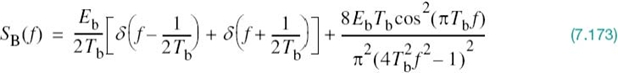
From Chapter 4, we recall the following relationship between baseband modulated power spectra:

where f_c is the carrier frequency. Therefore, substituting (7.173) into (7.174), we find that the power spectrum of the binary FSK signal contains two discrete frequency components, one located at (f_c + 1/2T_b) = f₁ and the other located at (f_c – 1/2T_b) = f₂, with their average powers adding up to one-half the total power of the binary FSK signal. The presence of these two discrete frequency components serves a useful purpose: it provides a practical basis for synchronizing the receiver with the transmitter.

Examining (7.173), we may make the following statement:

The baseband power spectral density of a binary FSK signal with continuous phase ultimately falls off as the inverse fourth power of frequency.

In Figure 7.15, we plotted the baseband power spectra of (7.111) and (7.173). (To simplify matters, we have only plotted the results for positive frequencies.) In both cases, S_B(f) is shown normalized with respect to 2E_b, and the frequency is normalized with respect to the bit rate R_b = 1/T_b. The difference in the falloff rates of these spectra can be explained on the basis of the pulse shape g(t). The smoother the pulse, the faster the drop of spectral tails to zero. Thus, since binary FSK with continuous phase has a smoother pulse shape, it has lower sidelobes than binary PSK does.

Suppose, next, the FSK signal exhibits phase discontinuity at the inter-bit switching instants, which arises when the two oscillators supplying the basis functions with frequencies f₁ and f₂ operate independently of each other. In this discontinuous scenario, we find that power spectral density ultimately falls off as the inverse square of frequency. Accordingly, we may state:

A binary FSK signal with continuous phase does not produce as much interference outside the signal band of interest as a corresponding FSK signal with discontinuous phase does.

The important point to take from this statement is summed up as follows: when interference is an issue of practical concern, continuous FSK is preferred over its discontinuous counterpart. However, this advantage of continuous FSK is gained at the expense of increased system complexity.

Minimum Shift Keying

In the coherent detection of binary FSK signal, the phase information contained in the received signal is not fully exploited, other than to provide for synchronization of the receiver to the transmitter. We now show that by proper use of the continuous-phase property when performing detection it is possible to improve the noise performance of the receiver significantly. Here again, this improvement is achieved at the expense of increased system complexity.

Consider a continuous-phase frequency-shift keying (CPFSK) signal, which is defined for the signaling interval 0 ≤ t 0 ≤ T_b as follows:

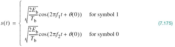
where E_b is the transmitted signal energy per bit and T_b is the bit duration. The defining equation (7.175) distinguishes itself from that of (7.151) in using the phase θ(0). This new term, denoting the value of the phase at time t = 0, sums up the past history of the FM process up to time t = 0. The frequencies f₁ and f₂ are sent in response to binary symbols 1 and 0, respectively, applied to the modulator input.

Another useful way of representing the CPFSK signal s(t) is to express it as a conventional angle-modulated signal:

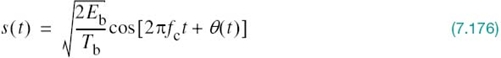
where θ(t) is the phase of s(t) at time t. When the phase θ(t) is a continuous function of time, we find that the modulated signal s(t) is itself also continuous at all times, including the inter-bit switching times. The phase θ(t) of a CPFSK signal increases or decreases linearly with time during each bit duration of T_b seconds, as shown by

where the plus sign corresponds to sending symbol 1 and the minus sign corresponds to sending symbol 0; the dimensionless parameter h is to be defined. Substituting (7.177) into (7.176), and then comparing the angle of the cosine function with that of (7.175), we deduce the following pair of relations:

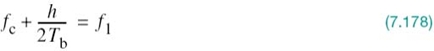
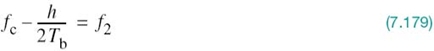
Solving this pair of equations for f_c and h, we get

and

The nominal carrier frequency f_c is, therefore, the arithmetic mean of the transmitted frequencies f₁ and f₂. The difference between the frequencies f₁ and f₂, normalized with respect to the bit rate 1/T_b, defines the dimensionless parameter h, which is referred to as the deviation ratio.

Phase Trellis

From (7.177) we find that, at time t = T_b,

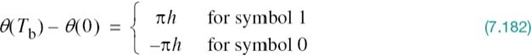
That is to say, sending symbol 1 increases the phase of a CPFSK signal s(t) by πh radians, whereas sending symbol 0 reduces it by an equal amount.

The variation of phase θ(t) with time t follows a path consisting of a sequence of straight lines, the slopes of which represent frequency changes. Figure 7.27 depicts possible paths starting from t = 0. A plot like that shown in this figure is called a phase tree. The tree makes clear the transitions of phase across successive signaling intervals. Moreover, it is evident from the figure that the phase of a CPFSK signal is an odd or even multiple of πh radians at odd or even multiples of the bit duration T_b, respectively.

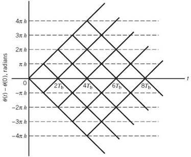
Figure 7.27 Phase tree.

The phase tree described in Figure 7.27 is a manifestation of phase continuity, which is an inherent characteristic of a CPFSK signal. To appreciate the notion of phase continuity, let us go back for a moment to Sunde’s FSK, which is also a CPFSK signal as previously described. In this case, the deviation ratio h is exactly unity. Hence, according to Figure 7.27, the phase change over one bit interval is ±π radians. But, a change of +π radians is exactly the same as a change of –π radians, modulo 2π. It follows, therefore, that in the case of Sunde’s FSK there is no memory; that is, knowing which particular change occurred in the previous signaling interval provides no help in the current signaling interval.

In contrast, we have a completely different situation when the deviation ratio h is assigned the special value of 1/2. We now find that the phase can take on only the two values ±π/2 at odd multiples of T_b, and only the two values 0 and π at even multiples of T_b, as in Figure 7.28. This second graph is called a phase trellis, since a “trellis” is a treelike structure with re-emerging branches. Each path from left to right through the trellis of Figure 7.28 corresponds to a specific binary sequence at the transmitter input. For example, the path shown in boldface in Figure 7.28 corresponds to the binary sequence 1101000 with θ(0) = 0. Henceforth, we focus on h = 1/2.

With h = 1/2, we find from (7.181) that the frequency deviation (i.e., the difference between the two signaling frequencies f₁ and f₂) equals half the bit rate; hence the following statement:

The frequency deviation h = 1/2 is the minimum frequency spacing that allows the two FSK signals representing symbols 1 and 0 to be coherently orthogonal.

In other words, symbols 1 and 0 do not interfere with one another in the process of detection. It is for this reason that a CPFSK signal with a deviation ratio of one-half is commonly referred to as minimum shift-keying (MSK).⁵

Signal-Space Diagram of MSK

Using a well-known trigonometric identity in (7.176), we may expand the CPFSK signal s(t) in terms of its in-phase and quadrature components as

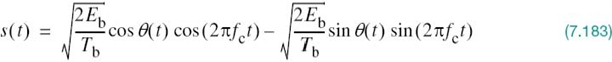
Consider, first, the in-phase component . With the deviation ratio h = 1/2, we have from (7.177) that

where the plus sign corresponds to symbol 1 and the minus sign corresponds to symbol 0. A similar result holds for θ(t) in the interval –T_b ≤ t ≤ 0, except that the algebraic sign is not necessarily the same in both intervals. Since the phase θ(0) is 0 or π depending on the past history of the modulation process, we find that in the interval –T_b ≤ t ≤ T_b, the polarity of cosθ(t) depends only on θ(0), regardless of the sequence of 1s and 0s transmitted before or after t = 0. Thus, for this time interval, the in-phase component consists of the half-cycle cosine pulse:

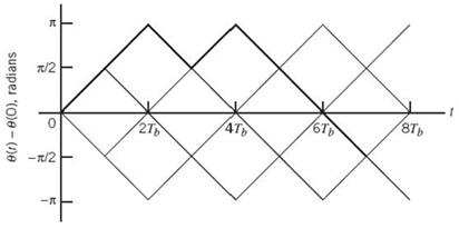
Figure 7.28 Phase trellis; boldfaced path represents the sequence 1101000.

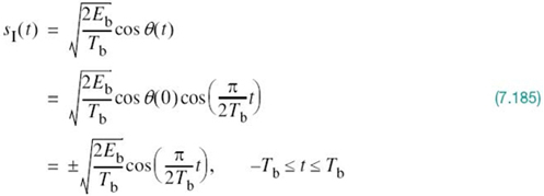
where the plus sign corresponds to θ(0) = 0 and the minus sign corresponds to θ(0) = π. In a similar way, we may show that, in the interval 0 ≤ t ≤ 2T_b, the quadrature component of s(t) consists of the half-cycle sine pulse:

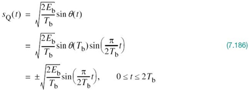
where the plus sign corresponds to θ(T_b) = π/2 and the minus sign corresponds to θ(T_b) = –π/2. From the discussion just presented, we see that the in-phase and quadrature components of the MSK signal differ from each other in two important respects:

• they are in phase quadrature with respect to each other and
• the polarity of the in-phase component s_I(t) depends on θ(0), whereas the polarity of the quadrature component s_Q(t) depends on θ(T_b).

Moreover, since the phase states θ(0) and θ(T_b) can each assume only one of two possible values, any one of the following four possibilities can arise:

1.  θ(0) = 0 and θ(T_b) = π/2, which occur when sending symbol 1.

2.  θ(0) = π and θ(T_b) = π/2, which occur when sending symbol 0.

3.  θ(0) = π and θ(T_b) = –π/2 (or, equivalently, 3π/2 modulo 2π), which occur when sending symbol 1.

4.  θ(0) = 0 and θ(T_b) = –π/2, which occur when sending symbol 0.

This fourfold scenario, in turn, means that the MSK signal itself can assume one of four possible forms, depending on the values of the phase-state pair: θ(0) and θ(T_b).

Signal-Space Diagram

Examining the expansion of (7.183), we see that there are two orthonormal basis functions ϕ₁(t) and ϕ₂(t) characterizing the generation of MSK; they are defined by the following pair of sinusoidally modulated quadrature carriers:

With the formulation of a signal-space diagram in mind, we rewrite (7.183) in the compact form

where the coefficients s₁ and s₂ are related to the phase states θ(0) and θ(T_b), respectively. To evaluate s₁, we integrate the product s(t)ϕ₁(t) with respect to time t between the limits –T_b and T_b, obtaining

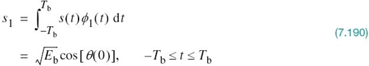
Similarly, to evaluate s₂ we integrate the product s(t)ϕ₂(t) with respect to time t between the limits 0 and 2T_b, obtaining

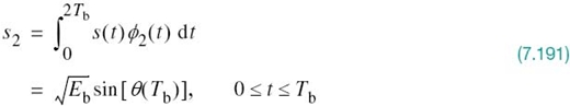
Examining (7.190) and (7.191), we now make three observations:

1.  Both integrals are evaluated for a time interval equal to twice the bit duration.

2.  The lower and upper limits of the integral in (7.190) used to evaluate s₁ are shifted by the bit duration T_b with respect to those used to evaluate s₂.

3.  The time interval 0 ≤ t ≤ T_b, for which the phase states θ(0) and θ(T_b) are defined, is common to both integrals.

It follows, therefore, that the signal constellation for an MSK signal is two-dimensional (i.e., N = 2), with four possible message points (i.e., M = 4), as illustrated in the signal-space diagram of Figure 7.29. Moving in a counterclockwise direction, the coordinates of the message points are as follows:

The possible values of θ(0) and θ(T_b), corresponding to these four message points, are also included in Figure 7.29. The signal-space diagram of MSK is thus similar to that of QPSK in that both of them have four message points in a two-dimensional space. However, they differ in a subtle way that should be carefully noted:

• QPSK, moving from one message point to an adjacent one, is produced by sending a two-bit symbol (i.e., dibit).
• MSK, on the other hand, moving from one message point to an adjacent one, is produced by sending a binary symbol, 0 or 1. However, each symbol shows up in two opposite quadrants, depending on the value of the phase-pair: θ(0) and θ(T_b).

Table 7.4 presents a summary of the values of θ(0) and θ(T_b), as well as the corresponding values of s₁ and s₂ that are calculated for the time intervals –T_b ≤ t ≤ T_b and 0 ≤ t ≤ 2T_b, respectively. The first column of this table indicates whether symbol 1 or symbol 0 was sent in the interval 0 ≤ t ≤ T_b. Note that the coordinates of the message points, s₁ and s₂, have opposite signs when symbol 1 is sent in this interval, but the same sign when symbol 0 is sent. Accordingly, for a given input data sequence, we may use the entries of Table 7.4 to derive on a bit-by-bit basis the two sequences of coefficients required to scale ϕ₁(t) and ϕ₂(t), and thereby determine the MSK signal s(t).

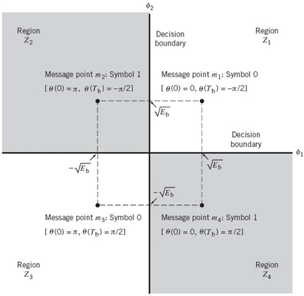
Figure 7.29 Signal-space diagram for MSK system.

Table 7.4 Signal-space characterization of MSK

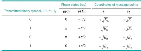
EXAMPLE 8   MSK Waveforms

Figure 7.30 shows the sequences and waveforms involved in the generation of an MSK signal for the binary sequence 1101000. The input binary sequence is shown in Figure 7.30a. The two modulation frequencies are f₁ = 5/4T_b and f₂ = 3/4T_b. Assuming that at time t = 0 the phase θ(0) is zero, the sequence of phase states is as shown in Figure 7.30, modulo 2π. The polarities of the two sequences of factors used to scale the time functions ϕ₁(t) and ϕ₂(t) are shown in the top lines of Figure 7.30b and c. These two sequences are offset relative to each other by an interval equal to the bit duration T_b. The waveforms of the resulting two components of s(t), namely, s₁ϕ₁(t) and s₂ϕ₂(t), are shown in Figure 7.30b and c. Adding these two modulated waveforms, we get the desired MSK signal s(t) shown in Figure 7.30d.

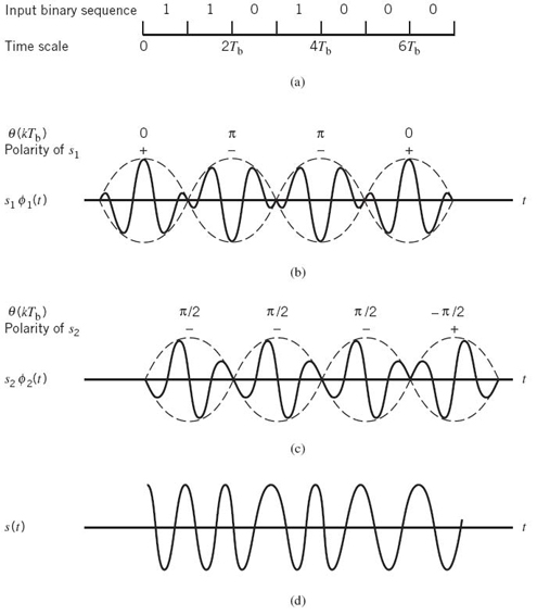
Figure 7.30 (a) Input binary sequence. (b) Waveform of scaled time function s₁ϕ₁(t). (c) Waveform of scaled time function s₂ϕ₂(t). (d) Waveform of the MSK signal s(t) obtained by adding s₁ϕ₁(t) and s₂ϕ₂(t) on a bit-by-bit basis.

Generation and Coherent Detection of MSK Signals

With h = 1/2, we may use the block diagram of Figure 7.31a to generate the MSK signal. The advantage of this method of generating MSK signals is that the signal coherence and deviation ratio are largely unaffected by variations in the input data rate. Two input sinusoidal waves, one of frequency f_c = n_c/4T_b for some fixed integer n_c and the other of frequency 1/4T_b, are first applied to a product modulator. This modulator produces two phase-coherent sinusoidal waves at frequencies f₁ and f₂, which are related to the carrier frequency f_c and the bit rate 1/T_b in accordance with (7.178) and (7.179) for deviation ratio h = 1/2. These two sinusoidal waves are separated from each other by two narrowband filters, one centered at f₁ and the other at f₂. The resulting filter outputs are next linearly combined to produce the pair of quadrature carriers or orthonormal basis functions ϕ₁(t) and ϕ₂(t). Finally, a₁(t) and a₂(t) are multiplied with two binary waves a₁(t) and a₂(t), both of which have a bit rate equal to 1/(2T_b). These two binary waves are extracted from the incoming binary sequence in the manner described in Example 7.

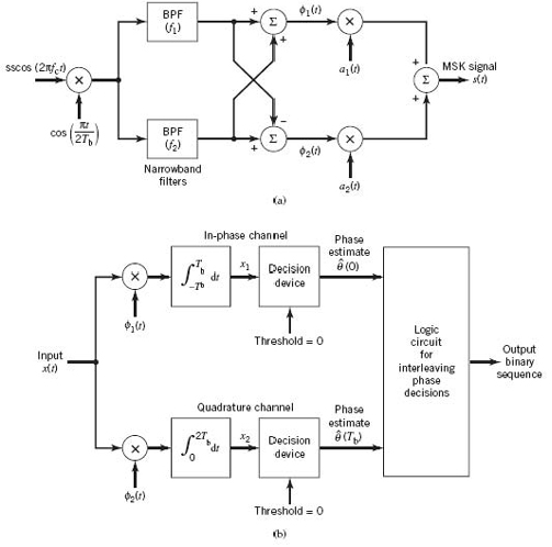
Figure 7.31 Block diagrams for (a) MSK transmitter and (b) coherent MSK receiver.

Figure 7.31b shows the block diagram of the coherent MSK receiver. The received signal x(t) is correlated with ϕ₁(t) and ϕ₂(t). In both cases, the integration interval is 2T_b seconds, and the integration in the quadrature channel is delayed by T_b seconds with respect to that in the in-phase channel. The resulting in-phase and quadrature channel correlator outputs, x₁ and x₂, are each compared with a threshold of zero; estimates of the phase θ(0) and θ(T_b) are then derived in the manner described previously. Finally, these phase decisions are interleaved so as to estimate the original binary sequence at the transmitter input with the minimum average probability of symbol error in an AWGN channel.

Error Probability of MSK

In the case of an AWGN channel, the received signal is given by

where s(t) is the transmitted MSK signal and w(t) is the sample function of a white Gaussian noise process of zero mean and power spectral density N₀/2. To decide whether symbol 1 or symbol 0 was sent in the interval 0 ≤ t ≤ T_b, say, we have to establish a procedure for the use of x(t) to detect the phase states θ(0) and θ(T_b).

For the optimum detection of θ(0), we project the received signal x(t) onto the reference signal ϕ₁(t) over the interval –T_b ≤ t ≤ T_b, obtaining

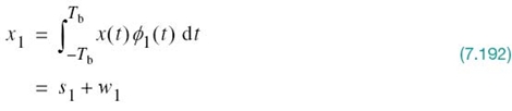
where s₁ is as defined by (7.190) and w₁ is the sample value of a Gaussian random variable of zero mean and variance N₀/2. From the signal-space diagram of Figure 7.29, we see that if x₁ > 0, the receiver chooses the estimate θ̂(0). On the other hand, if x₁ < 0, it chooses the estimate θ̂(0) = π.

Similarly, for the optimum detection of θ(T_b), we project the received signal x(t) onto the second reference signal ϕ₂(t) over the interval 0 ≤ t ≤ 2T_b, obtaining

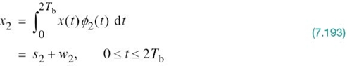
where s₂ is as defined by (7.191) and w₂ is the sample value of another independent Gaussian random variable of zero mean and variance N₀/2. Referring again to the signal-space diagram of Figure 7.29, we see that if x₂ . 0, the receiver chooses the estimate θ(T_b) = –π/2. If, however, x₂ , 0, the receiver chooses the estimate θ̂(T_b) = π/2.

To reconstruct the original binary sequence, we interleave the above two sets of phase estimates in accordance with Table 7.4, by proceeding as follows:

• If estimates θ̂(0) = 0 and θ̂(0) = (T_b) = –π/2, or alternatively if θ̂(0) and, θ̂(T_b) = –π/2, then the receiver decides in favor of symbol 0.
• If, on the other hand, the estimates θ̂(0) = π and θ̂(T_b) = –π/2, or alternatively if θ̂(0) = 0; and, θ̂(T_b) = –π/2, then the receiver decides in favor of symbol 1.

Most importantly, examining the signal-space diagram of Figure 7.29, we see that the coordinates of the four message points characterizing the MSK signal are identical to those of the QPSK signal in Figure 7.16. Moreover, the zero-mean noise variables in (7.192) and (7.193) have exactly the same variance as those for the QPSK signal in (7.118) and (7.119). It follows, therefore, that the BER for the coherent detection of MSK signals is given by

which is the same as that of QPSK in (7.126). In both MSK and QPSK, this good performance is the result of coherent detection being performed in the receiver on the basis of observations over 2T_b seconds.

Power Spectra of MSK Signals

As with the binary FSK signal, we assume that the input binary wave is random, with symbols 1 and 0 being equally likely and the symbols sent during adjacent time slots being statistically independent. Under these assumptions, we make three observations:

1.  Depending on the value of phase state θ(0), the in-phase component equals +g(t) or –g(t), where the pulse-shaping function

The energy spectral density of g(t) is

The power spectral density of the in-phase component equals ψ_g(f)/2T_b.

2.  Depending on the value of the phase state θ(T_b), the quadrature component equals +g(t) or –g(t), where we now have

Despite the difference in which the time interval over two adjacent time slots is defined in (7.195) and (7.197), we get the same energy spectral density as in (7.196).

Hence, the in-phase and quadrature components have the same power spectral density.

3.  The in-phase and quadrature components of the MSK signal are statistically independent; it follows that the baseband power spectral density of s(t) is given by

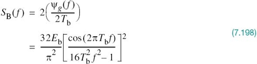
A plot of the baseband power spectrum of (7.198) is included in Figure 7.19, where the power spectrum is normalized with respect to 4E_b and the frequency f is normalized with respect to the bit rate 1/T_b. Figure 7.19 also includes the corresponding plot of (7.128) for the QPSK signal. As stated previously, for f ≫1/T_b the baseband power spectral density of the MSK signal falls off as the inverse fourth power of frequency, whereas in the case of the QPSK signal it falls off as the inverse square of frequency. Accordingly, MSK does not produce as much interference outside the signal band of interest as QPSK does. This is a desirable characteristic of MSK, especially when the digital communication system operates with a bandwidth limitation in an interfering environment.

Gaussian-Filtered MSK

From the detailed study of MSK just presented, we may summarize its desirable properties:

• modulated signal with constant envelope;
• relatively narrow-bandwidth occupancy;
• coherent detection performance equivalent to that of QPSK.

However, the out-of-band spectral characteristics of MSK signals, as good as they are, still do not satisfy the stringent requirements of certain applications such as wireless communications. To illustrate this limitation, we find from (7.198) that, at T_b f = 0.5, the baseband power spectral density of the MSK signal drops by only 10 log₁₀9 = 9.54 dB below its mid-band value. Hence, when the MSK signal is assigned a transmission bandwidth of 1/T_b, the adjacent channel interference of a wireless-communication system using MSK is not low enough to satisfy the practical requirements of a multiuser-communications environment.

Recognizing that the MSK signal can be generated by direct FM of a voltage-controlled oscillator, we may overcome this practical limitation of MSK by modifying its power spectrum into a more compact form while maintaining the constant-envelope property of the MSK signal. This modification can be achieved through the use of a premodulation low-pass filter, hereafter referred to as a baseband pulse-shaping filter. Desirably, the pulse-shaping filter should satisfy the following three conditions:

• frequency response with narrow bandwidth and sharp cutoff characteristics;
• impulse response with relatively low overshoot; and
• evolution of a phase trellis with the carrier phase of the modulated signal assuming the two values ±π/2 at odd multiples of the bit duration T_b and the two values 0 and π at even multiples of T_b as in MSK.

The frequency-response condition is needed to suppress the high-frequency components of the modified frequency-modulated signal. The impulse-response condition avoids excessive deviations in the instantaneous frequency of the modified frequency-modulated signal. Finally, the condition imposed on phase-trellis evolution ensures that the modified frequency-modulated signal can be coherently detected in the same way as the MSK signal, or it can be noncoherently detected as a simple binary FSK signal if so desired.

These three conditions can be satisfied by passing an NRZ-level-encoded binary data stream through a baseband pulse-shaping filter whose impulse response (and, likewise, its frequency response) is defined by a Gaussian function. The resulting method of binary FM is naturally referred to as Gaussian-filtered minimum-shift keying (GMSK).⁶

Let W denote the 3 dB baseband bandwidth of the pulse-shaping filter. We may then define the transfer function H(f) and impulse response h(t) of the pulse-shaping filter as:

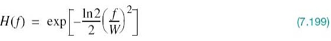
and

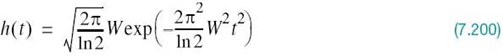
where ln denotes the natural algorithm. The response of this Gaussian filter to a rectangular pulse of unit amplitude and duration T_b, centered on the origin, is given by

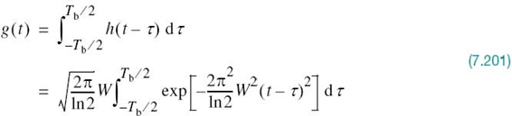
The pulse response g(t) in (7.201) provides the basis for building the GMSK modulator, with the dimensionless time–bandwidth product WT_b playing the role of a design parameter.

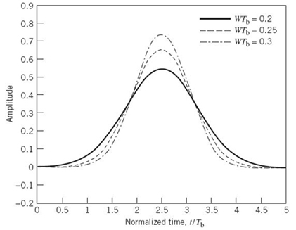
Figure 7.32 Frequency-shaping pulse g(t) of (7.201) shifted in time by 2.5T_b and truncated at ±2.5T_b for varying time–bandwidth product WT_b.

Unfortunately, the pulse response g(t) is noncausal and, therefore, not physically realizable for real-time operation. Specifically, g(t) is nonzero for t , –T_b/2, where t = –T_b/2 is the time at which the input rectangular pulse (symmetrically positioned around the origin) is applied to the Gaussian filter. For a causal response, g(t) must be truncated and shifted in time. Figure 7.32 presents plots of g(t), which has been truncated at t = ±2.5T_b and then shifted in time by 2.5T_b. The plots shown here are for three different settings: WT_b = 0.2, 0.25, and 0.3. Note that as WT_b is reduced, the time spread of the frequency-shaping pulse is correspondingly increased.

Figure 7.33 shows the machine-computed power spectra of MSK signals (expressed in decibels) versus the normalized frequency difference (f – f_c)T_b, where f_c is the mid-band frequency and T_b is the bit duration.⁷ The results plotted in Figure 7.33 are for varying values of the time–bandwidth product WT_b. From this figure we may make the following observations:

• The curve for the limiting condition WT_b corresponds to the case of ordinary MSK.
• When WT_b is less than unity, increasingly more of the transmit power is concentrated inside the passband of the GMSK signal.

An undesirable feature of GMSK is that the processing of NRZ binary data by a Gaussian filter generates a modulating signal that is no longer confined to a single bit interval as in ordinary MSK, which is readily apparent from Figure 7.33. Stated in another way, the tails of the Gaussian impulse response of the pulse-shaping filter cause the modulating signal to spread out to adjust symbol intervals. The net result is the generation of intersymbol interference, the extent of which increases with decreasing WT_b. In light of this discussion and the various plots presented in Figure 7.33, we find that the value assigned to the time-bandwidth product WT_b offers a tradeoff between spectral compactness and system-performance loss.

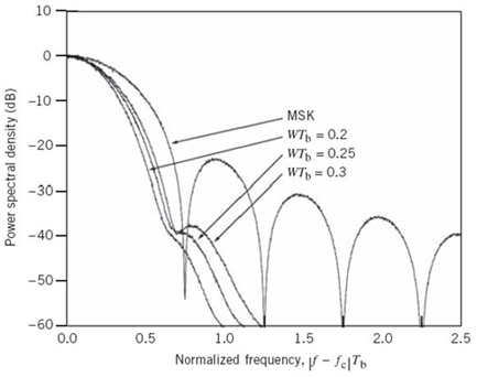
Figure 7.33 Power spectra of MSK and GMSK signals for varying time–bandwidth product.

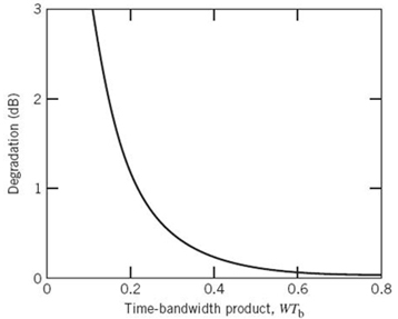
Figure 7.34 Theoretical E_b/N₀ degradation of GMSK for varying time–bandwidth product.

To explore the issue of performance degradation resulting from the use of GMSK compared with MSK, consider the coherent detection in the presence of AWGN. Recognizing that GMSK is a special kind of binary FM, we may express its average probability of symbol error P_e by the empirical formula

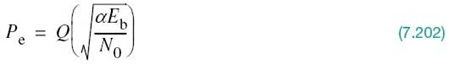
where, as before, E_b is the signal energy per bit and N₀/2 is the noise spectral density. The factor α is a constant whose value depends on the time–bandwidth product WT_b. Comparing (7.202) for GMSK with (7.194) for ordinary MSK, we may view 10 log₁₀(α/2), expressed indecibels, as a measure of performance degradation of GMSK compared with ordinary MSK. Figure 7.34 shows the machine-computed value of 10 log₁₀(Ρ/2) versus WT_b. For ordinary MSK we have, in which case (7.202) with α = 2 assumes exactly the same form as (7.194) and there is no degradation in performance, which is confirmed by Figure 7.34. For GMSK with WT_b = 0.3 we find from Figure 7.34 that there is a degradation in performance of about 0.46dB, which corresponds to α/2 = 0.9. This degradation in performance is a small price to pay for the highly desirable spectral compactness of the GMSK signal.

M-ary FSK

Consider next the M-ary version of FSK, for which the transmitted signals are defined by

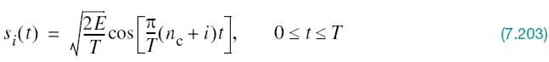
where i = 1,2,…,M, and the carrier frequency f_c = n_c/(2T) for some fixed integer n_c. The transmitted symbols are of equal duration T and have equal energy E. Since the individual signal frequencies are separated by 1/(2T) Hz, the M-ary FSK signals in (7.203) constitute an orthogonal set; that is,

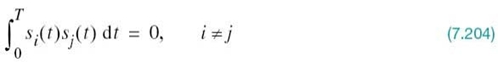
Hence, we may use the transmitted signals s_i(t) themselves, except for energy normalization, as a complete orthonormal set of basis functions, as shown by

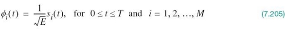
Accordingly, the M-ary FSK is described by an M-dimensional signal-space diagram.

For the coherent detection of M-ary FSK signals, the optimum receiver consists of a bank of M correlators or matched filters, with ϕ_i(t) of (7.205) providing the basis functions. At the sampling times t = kT, the receiver makes decisions based on the largest matched filter output in accordance with the maximum likelihood decoding rule. An exact formula for the probability of symbol error is, however, difficult to derive for a coherent M-ary FSK system. Nevertheless, we may use the union bound of (7.88) to place an upper bound on the average probability of symbol error for M-ary FSK. Specifically, since the minimum distance d_min in M-ary FSK is, using (7.87) we get (assuming equiprobable symbols)

For fixed M, this bound becomes increasingly tight as the ratio E/N₀ is increased. Indeed, it becomes a good approximation to P_e for values of P_e ≤ 10^–3. Moreover, for M = 2 (i.e., binary FSK), the bound of (7.202) becomes an equality; see (7.168).

Power Spectra of M-ary FSK Signals

The spectral analysis of M-ary FSK signals⁸ is much more complicated than that of M-ary PSK signals. A case of particular interest occurs when the frequencies assigned to the multilevels make the frequency spacing uniform and the frequency deviation h = 1/2. That is, the M signal frequencies are separated by 1/2T, where T is the symbol duration. For h = 1/2, the baseband power spectral density of M-ary FSK signals is plotted in Figure 7.35 for M = 2, 4, 8.

Bandwidth Efficiency of M-ary FSK Signals

When the orthogonal signals of an M-ary FSK signal are detected coherently, the adjacent signals need only be separated from each other by a frequency difference 1/2T so as to maintain orthogonality. Hence, we may define the channel bandwidth required to transmit M-ary FSK signals as

For multilevels with frequency assignments that make the frequency spacing uniform and equal to 1/2T, the bandwidth B of (7.207) contains a large fraction of the signal power.

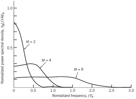
Figure 7.35 Power spectra of M-ary PSK signals for M = 2, 4, 8.

This is readily confirmed by looking at the baseband power spectral plots shown in Figure 7.36. From (7.133) we recall that the symbol period T is equal to T_b log₂ M. Hence, using R_b = 1/T^b, we may redefine the channel bandwidth B for M-ary FSK signals as

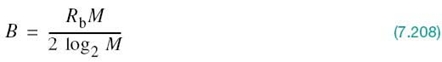
The bandwidth efficiency of M-ary signals is therefore

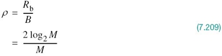
Table 7.5 gives the values of ρ calculated from (7.207) for varying M.

Comparing Tables 7.3 and 7.5, we see that increasing the number of levels M tends to increase the bandwidth efficiency of M-ary PSK signals, but it also tends to decrease the bandwidth efficiency of M-ary FSK signals. In other words, M-ary PSK signals are spectrally efficient, whereas M-ary FSK signals are spectrally inefficient.

Table 7.5 Bandwidth efficiency of M-ary FSK signals

7.9 Comparison of M-ary PSK and M-ary FSK from an Information-Theoretic Viewpoint

Bandwidth efficiency, as just discussed, provides one way of contrasting the capabilities of M-ary PSK and M-ary FSK. Another way of contrasting the capabilities of these two generalized digital modulation schemes is to look at the bandwidth–power tradeoff viewed in light of Shannon’s information capacity law, which was discussed previously in Chapter 5.

Consider, first, an M-ary PSK system that employs a nonorthogonal set of M phase-shifted signals for the transmission of binary data over an AWGN channel. Referring back to Section 7.6, recall that (7.137) defines the bandwidth efficiency of the M-ary PSK system, using the null-to-null bandwidth. Based on this equation, Figure 7.36 plots the operating points for different phase-level numbers M = 2, 4, 8, 16, 32, 64. Each point on the operating curve corresponds to an average probability of symbol error P_e = 10^–5; this value of P_e is small enough to assume “error-free” transmission. Given this fixed value of P_e, (7.132) for the coherent detection of M-ary PSK is used to calculate the symbol energy-to-noise density ratio E/N₀ and, therefore, E_b/N₀ for a prescribed M; Figure 7.36 also includes the capacity boundary for the ideal transmission system, computed in accordance with (5.99). Figure 7.36 teaches us the following:

In M-ary PSK using coherent detection, increasing M improves the bandwidth efficiency, but the E_b/N₀ required for the idealized condition of “error-free” transmission moves away from the Shannon limit as M is increased.

Consider next an M-ary FSK system that uses an orthogonal set of M frequency-shifted signals for the transmission of binary data over an AWGN channel. As discussed in Section 7.8, the separation between adjacent signal frequencies in the set is 1/2T, where T is the symbol period. The bandwidth efficiency of M-ary FSK is defined in (7.209), the formulation of which also invokes the null-to-null bandwidth. Using this equation, Figure 7.37 plots the operating points for different frequency-level numbers M = 2, 4, 8, 16, 32, 64 for the same average probability of symbol error, namely P_e = 10^–5. Given this fixed value of P_e, (7.206) is used to calculate the E/N₀ and, therefore, E_b/N₀ required for a prescribed value of M. As in Figure 7.36 for M-ary PSK, Figure 7.37 for M-ary FSK also includes the capacity boundary for the ideal condition of error-free transmission. Figure 7.37 shows that increasing M in M-ary FSK has the opposite effect to that in M-ary PSK. In more specific terms, we may state the following:

In M-ary FSK, as the number of frequency-shift levels M is increased—which is equivalent to increased channel-bandwidth requirement—the operating point moves closer to the Shannon limit.

In other words, in an information-theoretic context, M-ary FSK behaves better than M-ary PSK.

In the final analysis, the choice of M-ary PSK or M-ary FSK for binary data transmission over an AWGN channel is determined by the design criterion of interest: bandwidth efficiency or the E_b/N₀ needed for reliable data transmission.

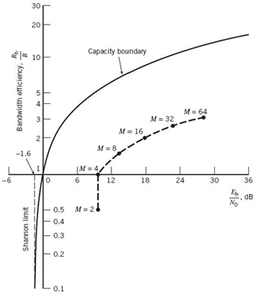
Figure 7.36 Comparison of M-ary PSK with the ideal system for P_e = 10^–5.

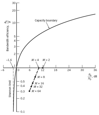
Figure 7.37 Comparison of M-ary FSK with the ideal system for P_e = 10^–5.

7.10  Detection of Signals with Unknown Phase

Up to this point in the chapter we have assumed that the receiver is perfectly synchronized to the transmitter and the only channel impairment is AWGN. In practice, however, it is often found that, in addition to the uncertainty due to channel noise, there is also uncertainty due to the randomness of certain signal parameters. The usual cause of this uncertainty is distortion in the transmission medium. Perhaps the most common random signal parameter is the carrier phase, which is especially true for narrowband signals. For example, the transmission may take place over a multiplicity of paths of different and variable length, or there may be rapidly varying delays in the propagating medium from transmitter to receiver. These sources of uncertainty may cause the phase of the received signal to change in a way that the receiver cannot follow. Synchronization with the phase of the transmitted carrier is then too costly and the designer may simply choose to disregard the phase information in the received signal at the expense of some degradation in noise performance. A digital communication receiver with no provision made for carrier phase recovery is said to be noncoherent.

Optimum Quadratic Receiver

Consider a binary communication system, in which the transmitted signal is defined by

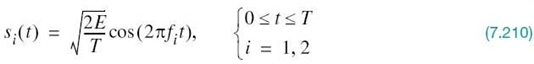
where E is the signal energy, T is the duration of the signaling interval, and the carrier frequency f_i for symbol i is an integer multiple of 1/(2T). For reasons just mentioned, the receiver operates noncoherently with respect to the transmitter, in which case the received signal for an AWGN channel is written as

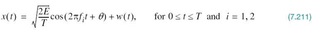
where θ is the unknown carrier phase and, as before, w(t) is the sample function of a white Gaussian noise process of zero mean and power spectral density N₀/2. Assuming complete lack of prior information about θ, we may treat it as the sample value of a random variable with uniform distribution:

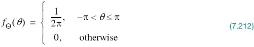
Such a distribution represents the worst-case scenario that could be encountered in practice. The binary detection problem to be solved may now be stated as follows:

Given the received signal x(t) and confronted with the unknown carrier phase θ, design an optimum receiver for detecting symbol s_i represented by the signal component that is contained in x(t).

Proceeding in a manner similar to that described in Section 7.4, we may formulate the likelihood function of symbol s_i given the carrier phase θ as

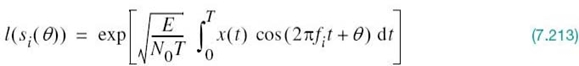
To proceed further, we have to remove dependence of l(s_i(θ)) on phase θ, which is achieved by integrating it over all possible values of θ, as shown by

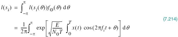
Using a well-known trigonometric formula, we may expand the cosine term in (7.214) as

Correspondingly, we may rewrite the integral in the exponent of (7.214) as

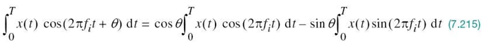
Define two new terms:

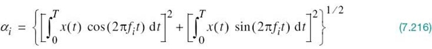
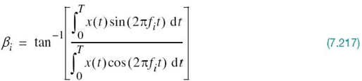
Then, we may go one step further and simplify the inner integral in (7.214) to

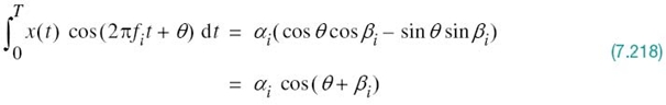
Accordingly, using (7.218) in (7.214), we obtain

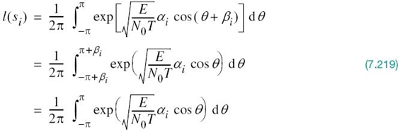
where, in the last line, we have used the fact that the definite integral is unaffected by the phase β_i.

From Appendix C on Bessel functions, we recognize the integral of (7.219) as the modified Bessel function of zero order, written in the compact form

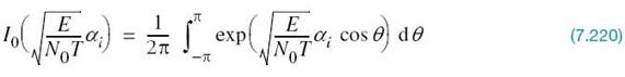
Using this formula, we may correspondingly express the likelihood function for the signal-detection problem described herein in the compact form

With binary transmission as the issue of interest, there are two hypotheses to be considered: hypothesis H₁, that signal s₁(t) was sent, and hypothesis H₂, that signal s₂ was sent. In light of (7.221), the binary-hypothesis test may now be formulated as follows:

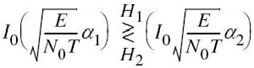
The modified Bessel function I(·) is a monotonically increasing function of its argument. Hence, we may simplify the hypothesis test by focusing on α_i for given E/N₀T. For convenience of implementation, however, the simplified hypothesis test is carried out interms of α_i² rather than α_i; that is to say:

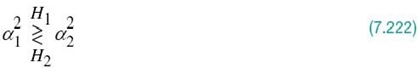
For obvious reasons, a receiver based on (7.222) is known as the quadratic receiver. In light of the definition of α_i given in (7.216), the receiver structure for computing α_i is as shown in Figure 7.38a. Since the test described in (7.222) is independent of the symbol energy E, this hypothesis test is said to be uniformly most powerful with respect to E.

Two Equivalent Forms of the Quadratic Receiver

We next derive two equivalent forms of the quadrature receiver shown in Figure 7.38a. The first form is obtained by replacing each correlator in this receiver with a corresponding equivalent matched filter. We thus obtain the alternative form of quadrature receiver shown in Figure 7.38b. In one branch of this receiver, we have a filter matched to the signal cos(2πf_it) and in the other branch we have a filter matched to sin(2πf_it), both of which are defined for the signaling interval 0 ≤ t ≤ T. At time t = T, the filter outputs are sampled, squared, and then added together.

To obtain the second equivalent form of the quadrature receiver, suppose we have a filter that is matched to s(t) = cos(2πf_it + θ) for 0 ≤ t ≤ T. The envelope of the matched filter output is obviously unaffected by the value of phase θ. Therefore, we may simply choose a matched filter with impulse response cos[2πf_i(T – t)], corresponding to θ = 0. The output of such a filter in response to the received signal x(t) is given by

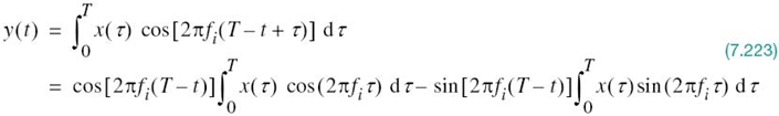
The envelope of the matched filter output is proportional to the square root of the sum of the squares of the two definite integrals in (7.223). This envelope, evaluated at time t = T, is, therefore, given by the following square root:

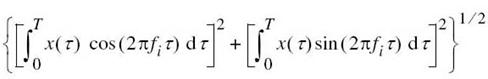
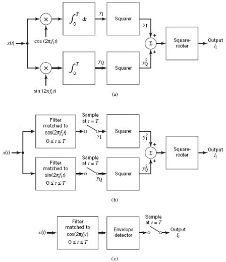
Figure 7.38 Noncoherent receivers: (a) quadrature receiver using correlators; (b) quadrature receiver using matched fiters; (c) noncoherent matched filter.

But this is just a repeat of the output of the quadrature receiver defined earlier. Therefore, the output (at time T) of a filter matched to the signal cos(2πf_it + θ) of arbitrary phase θ, followed by an envelope detector, is the same as the quadrature receiver’s output l_i. This form of receiver is shown in Figure 7.38c. The combination of matched filter and envelope detector shown in Figure 7.38c is called a noncoherent matched filter.

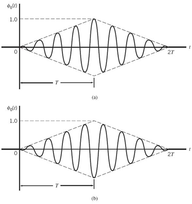
Figure 7.39 Output of matched filter for a rectangular RF wave: (a) ; (b).

The need for an envelope detector following the matched filter in Figure 7.38c may also be justified intuitively as follows. The output of a filter matched to a rectangular RF wave reaches a positive peak at the sampling instant t = T. If, however, the phase of the filter is not matched to that of the signal, the peak may occur at a time different from the sampling instant. In actual fact, if the phases differ by 180°, we get a negative peak at the sampling instant. Figure 7.39 illustrates the matched filter output for the two limiting conditions: θ = 0 and θ = 180° for which the respective waveforms of the matched filter output are displayed in parts a and b of the figure. To avoid poor sampling that arises in the absence of prior information about the phase, it is reasonable to retain only the envelope of the matched filter output, since it is completely independent of the phase mismatch θ.

7.11  Noncoherent Orthogonal Modulation Techniques

With the noncoherent receiver structures of Figure 7.38 at our disposal, we may now proceed to study the noise performance of noncoherent orthogonal modulation that includes two noncoherent receivers as special cases: noncoherent binary FSK; and differential PSK (called DPSK), which may be viewed as the noncoherent version of binary PSK.

Consider a binary signaling scheme that involves the use of two orthogonal signals s₁(t) and s₂(t), which have equal energy. During the signaling interval 0 ≤ t ≤ T, where T may be different from the bit duration T_b, one of these two signals is sent over an imperfect channel that shifts the carrier phase by an unknown amount. Let g₁(t) and g₂(t) denote the phase-shifted versions of s₁(t) and s₂(t) that result from this transmission, respectively. It is assumed that the signals g₁(t) and g₂(t) remain orthogonal and have the same energy E, regardless of the unknown carrier phase. We refer to such a signaling scheme as noncoherent orthogonal modulation, hence the title of the section.

In addition to carrier-phase uncertainty, the channel also introduces AWGN w(t) of zero mean and power spectral density N₀/2, resulting in the received signal

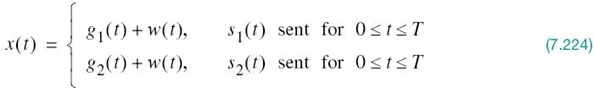
To tackle the signal detection problem given x(t), we employ the generalized receiver shown in Figure 7.39a, which consists of a pair of filters matched to the transmitted signals s₁(t) and s₂(t). Because the carrier phase is unknown, the receiver relies on amplitude as the only possible discriminant. Accordingly, the matched-filter outputs are envelope-detected, sampled, and then compared with each other. If the upper path in Figure 7.38a has an output amplitude l₁ greater than the output amplitude l₂ of the lower path, the receiver decides in favor of s₁(t); the l₁ and l₂ used here should not be confused with the symbol l denoting the likelihood function in the preceding section. If the converse is true, the receiver decides in favor of s₂(t). When they are equal, the decision may be made by flipping a fair coin (i.e., randomly). In any event, a decision error occurs when the matched filter that rejects the signal component of the received signal x(t) has a larger output amplitude (due to noise alone) than the matched filter that passes it.

From the discussion presented in Section 7.10 we note that a noncoherent matched filter (constituting the upper or lower path in the receiver of Figure 7.40a), may be viewed as being equivalent to a quadrature receiver. The quadrature receiver itself has two channels. One version of the quadrature receiver is shown in Figure 7.40b. In the upper path, called the in-phase path, the received signal x(t) is correlated with the function ψ_i(t), which represents a scaled version of the transmitted signal s₁(t) or s₂(t) with zero carrier phase. In the lower path, called the quadrature path on the other hand, x(t) is correlated with another function ψ̂_i(t), which represents the version of that results from shifting the carrier phase by –90°. The signals ψ_i(t) and ψ̂_i(t) are orthogonal to each other.

In actual fact, the signal ψ̂_i(t) is the Hilbert transform of ψ_i(t); the Hilbert transform was discussed in Chapter 2. To illustrate the nature of this relationship, let

where m(t) is a band-limited message signal. Typically, the carrier frequency f_i is greater than the highest frequency component of m(t). Then the Hilbert transform ψ_i(t) is defined by

for which reference should be made in Table 2.3 of Chapter 2. Since

we see that ψ̂_i(t) is indeed obtained from ψ_i(t) by shifting the carrier cos(2πf_it) by –90°. An important property of Hilbert transformation is that a signal and its Hilbert transform are orthogonal to each other. Thus, ψ_i(t) and ψ̂_i(t) are indeed orthogonal to each other, as already stated.

The average probability of error for the noncoherent receiver of Figure 7.40a is given by the simple formula

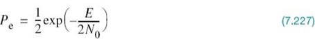
where E is the signal energy per symbol and N₀/2 is the noise spectral density.

Derivation of Equation (7.227)

To derive Equation (7.227)⁹ we make use of the equivalence depicted in Figure 7.40. In particular, we observe that, since the carrier phase is unknown, noise at the output of each matched filter in Figure 7.40a has two degrees of freedom: in-phase and quadrature. Accordingly, the noncoherent receiver of Figure 7.40a has a total of four noisy parameters that are conditionally independent given the phase θ, and also identically distributed. These four noisy parameters have sample values denoted by x_I1, x_Q1, and x_I2, and x_Q2; the first two account for degrees of freedom associated with the upper path of Figure 7.40a, and the latter two account for degrees of freedom associated with the lower path of the figure.

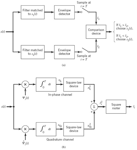
Figure 7.40 (a) Generalized binary receiver for noncoherent orthogonal modulation. (b) Quadrature receiver equivalent to either one of the two matched filters in (a); the index i = 1, 2.

The receiver of Figure 7.40a has a symmetric structure, meaning that the probability of choosing s₂(t) given that s₁(t) was transmitted is the same as the probability of choosing s₁(t) given that s₂(t) was transmitted. In other words, the average probability of error may be obtained by transmitting s₁(t) and calculating the probability of choosing s₂(t), or vice versa; it is assumed that the original binary symbols and therefore s₁(t) and s₂(t) are equiprobable.

Suppose that signal s₁(t) is transmitted for the interval 0 ≤ t ≤ T. An error occurs if the channel noise w(t) is such that the output l₂ of the lower path in Figure 7.40a is greater than the output l₁ of the upper path. Then, the receiver decides in favor of s₂(t) rather than s₁(t). To calculate the probability of error so made, we must have the probability density function of the random variable L₂ (represented by sample value l₂). Since the filter in the lower path is matched to s₂(t) and s₂(t) is orthogonal to the transmitted signal s₁(t), it follows that the output of this matched filter is due to noise alone. Let x_I2 and x_Q2 denote the in-phase and quadrature components of the matched filter output in the lower path of Figure 7.40a. Then, from the equivalent structure depicted in this figure, we see that (for i = 2)

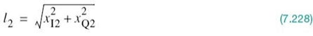
Figure 7.41a shows a geometric interpretation of this relation. The channel noise w(t) is both white (with power spectral density N₀/2) and Gaussian (with zero mean). Correspondingly, we find that the random variables X_I2 and X_Q2 (represented by sample values x_I2 and x_Q2) are both Gaussian distributed with zero mean and variance N₀/2, given the phase θ. Hence, we may write

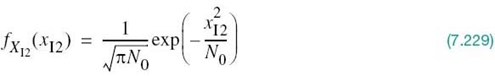
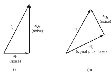
Figure 7.41 Geometric interpretations of the two path outputs l₁ and l₂ in the generalized non-coherent receiver.

and

Next, we use the well-known property presented in Chapter 4 on stochastic processes: the envelope of a Gaussian process represented in polar form is Rayleigh distributed and independent of the phase θ. For the situation at hand, therefore, we may state that the random variable L₂ whose sample value l₂ is related to x_I2 and x_Q2 by (7.228) has the following probability density function:

Figure 7.42 shows a plot of this probability density function, where the shaded area defines the conditional probability that l₂ > l₁. Hence, we have

Substituting (7.231) into (7.232) and integrating, we get

Consider next the output amplitude l₁, pertaining to the upper path in Figure 7.40a. Since the filter in this path is matched to s₁(t) and it is assumed that s₁(t) is transmitted, it follows that l₁ is due to signal plus noise. Let x_I1 and x_Q1 denote the components at the output of the matched filter in the upper path of Figure 7.39a that are in phase and in quadrature with respect to the received signal, respectively. Then, from the equivalent structure depicted in Figure 7.40b, we see that, for i = 1,

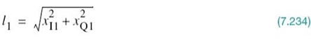
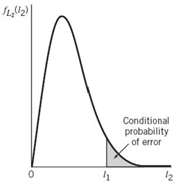
Figure 7.42 Calculation of the conditional probability that l₂ > l₁, given l₁.

A geometric interpretation of l_i is presented in Figure 7.41b. Since a Fourier-transformable signal and its Hilbert transform form an orthogonal pair, it follows that x_I1 is due to signal plus noise, whereas x_Q1 is due to noise alone. This statement has two implications:

• The random variable X_I1 represented by the sample value x_I1 is Gaussian distributed with mean and variance N₀/2, where E is the signal energy per symbol.
• The random variable X_Q1 represented by the sample value x_Q1 is Gaussian distributed with zero mean and variance N₀/2.

Hence, we may express the probability density functions of these two independent random variables as

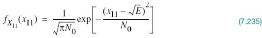
and

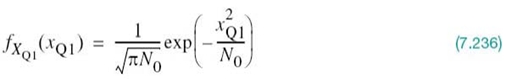
respectively. Since the two random variables X_I1 and X_Q1 are statistically independent, their joint probability density function is simply the product of the probability density functions given in (7.235) and (7.236).

To find the average probability of error, we have to average the conditional probability of error given in (7.233) over all possible values of l₁. Naturally, this calculation requires knowledge of the probability density function of random variables L₁ represented by sample value l₁. The standard method is now to combine (7.235) and (7.236) to find the probability density function of L₁ due to signal plus noise. However, this leads to rather complicated calculations involving the use of Bessel functions. This analytic difficulty may be circumvented by the following approach. Given x_I1 and x_Q1, an error occurs when, in Figure 7.40a, the lower path’s output amplitude l₂ due to noise alone exceeds l₁ due to signal plus noise; squaring both sides of (7.234), we write

The probability of the occurrence just described is obtained by substituting (7.237) into (7.233):

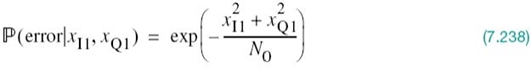
which is a probability of error conditioned on the output of the matched filter in the upper path of Figure 7.40a taking on the sample values x_I1 and x_Q1. This conditional probability multiplied by the joint probability density function of the random variables X_I1 and X_Q1 is the error-density given x_I1 and x_Q1. Since X_I1 and X_Q1 are statistically independent, their joint probability density function equals the product of their individual probability density functions. The resulting error-density is a complicated expression in x_I1 and x_Q1. However, the average probability of error, which is the issue of interest, may be obtained in a relatively simple manner. We first use (7.234), (7.235), and (7.236) to evaluate the desired error-density as

Completing the square in the exponent of (7.239) without the scaling factor –1/N₀, we may rewrite it as follows:

Next, we substitute (7.240) into (7.239) and integrate the error-density over all possible values of x_I1 and x_Q1, thereby obtaining the average probability of error:

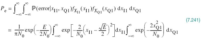
We now use the following two identities:

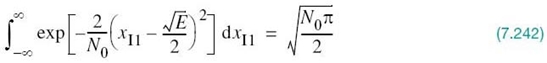
and

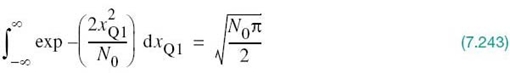
The identity of (7.242) is obtained by considering a Gaussian-distributed variable with mean and variance N₀/4 and recognizing the fact that the total area under the curve of a random variable’s probability density function is unity. The identity of (7.243) follows as a special case of (7.242). Thus, in light of these two identities, (7.241) reduces to

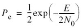
which is the desired result presented previously as (7.227). With this formula at our disposal, we are ready to consider noncoherent binary FSK and DPSK as special cases, which we do next in that order.¹⁰

7.12 Binary Frequency-Shift Keying Using Noncoherent Detection

In binary FSK, the transmitted signal is defined in (7.151) and repeated here for convenience of presentation:

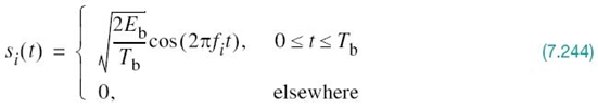
where T_b is the bit duration and the carrier frequency f_i equals one of two possible values f₁ and f₂; to ensure that the signals representing these two frequencies are orthogonal, we choose f_i = n_i/T_b, where n_i is an integer. The transmission of frequency f₁ represents symbol 1 and the transmission of frequency f₂ represents symbol 0. For the noncoherent detection of this frequency-modulated signal, the receiver consists of a pair of matched filters followed by envelope detectors, as in Figure 7.43. The filter in the upper path of the receiver is matched to cos(2πf₁t) and the filter in the lower path is matched to cos(2πf₂t) for the signaling interval 0 ≤ t ≤ T_b. The resulting envelope detector outputs are sampled at t = T_b and their values are compared. The envelope samples of the upper and lower paths in Figure 7.43 are shown as l₁ and l₂. The receiver decides in favor of symbol 1 if l₁ > l₂ and in favor of symbol 0 if l₁ < l₂. If l₁ = l₂, the receiver simply guesses randomly in favor of symbol 1 or 0.

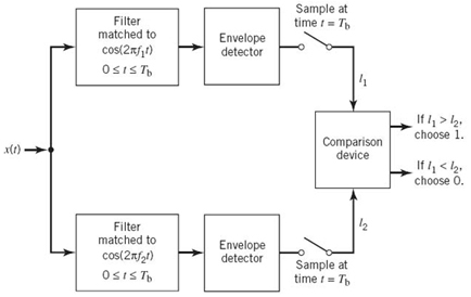
Figure 7.43 Noncoherent receiver for the detection of binary FSK signals.

The noncoherent binary FSK described herein is a special case of noncoherent orthogonal modulation with T = T_b and E = E_b, where E_b is the signal energy per bit. Hence, the BER for noncoherent binary FSK is

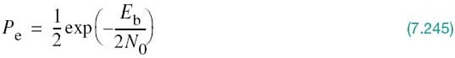
which follows directly from (7.227) as a special case of noncoherent orthogonal modulation.

7.13   Differential Phase-Shift Keying

As remarked at the beginning of Section 7.9, we may view DPSK as the “noncoherent” version of binary PSK. The distinguishing feature of DPSK is that it eliminates the need for synchronizing the receiver to the transmitter by combining two basic operations at the transmitter:

• differential encoding of the input binary sequence and
• PSK of the encoded sequence,

from which the name of this new binary signaling scheme follows.

Differential encoding starts with an arbitrary first bit, serving as the reference bit; to this end, symbol 1 is used as the reference bit. Generation of the differentially encoded sequence then proceeds in accordance with a two-part encoding rule as follows:

1.  If the new bit at the transmitter input is 1, leave the differentially encoded symbol unchanged with respect to the current bit.

2.  If, on the other hand, the input bit is 0, change the differentially encoded symbol with respect to the current bit.

The differentially encoded sequence, denoted by {d_k}, is used to shift the sinusoidal carrier phase by zero and 180^o, representing symbols 1 and 0, respectively. Thus, in terms of phase-shifts, the resulting DPSK signal follows the two-part rule:

1.  To send symbol 1, the phase of the DPSK signal remains unchanged.

2.  To send symbol 0, the phase of the DPSK signal is shifted by 180°.

EXAMPLE 9  Illustration of DPSK

Consider the input binary sequence, denoted {b_k}, to be 10010011, which is used to derive the generation of a DPSK signal. The differentially encoded process starts with the reference bit 1. Let {b_k} denote the differentially encoded sequence starting in this manner and {b_k-1} denote its delayed version by one bit. The complement of the modulo-2 sum of {b_k} and {b_k-1} defines the desired {b_k}, as illustrated in the top three lines of Table 7.6. In the last line of this table, binary symbols 1 and 0 are represented by phase-shifts of 1 and π radians.

Table 7.6 Illustrating the generation of DPSK signal

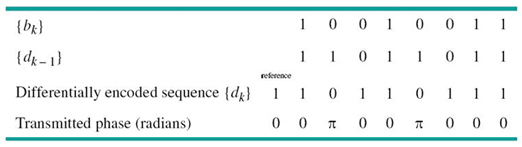
Error Probability of DPSK

Basically, the DPSK is also an example of noncoherent orthogonal modulation when its behavior is considered over successive two-bit intervals; that is, 0 ≤ t ≤ 2T_b. To elaborate, let the transmitted DPSK signal be for the first-bit interval 0 ≤ t ≤ T_b, which corresponds to symbol 1. Suppose, then, the input symbol for the second-bit interval is also symbol 1. According to part 1 of the DPSK encoding rule, the carrier phase remains unchanged, thereby yielding the DPSK signal

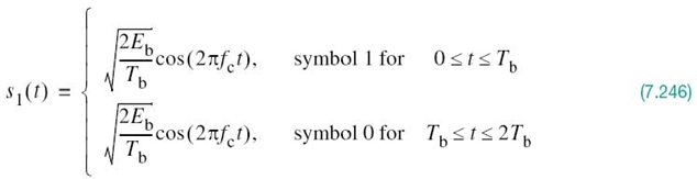
Suppose, next, the signaling over the two-bit interval changes such that the symbol at the transmitter input for the second-bit interval is 0. Then, according to part 2 of the DPSK encoding rule, the carrier phase is shifted by π radians (i.e., 180°), thereby yielding the new DPSK signal

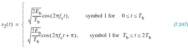
We now readily see from (7.246) and (7.247) that s₁(t) and s₂(t) are indeed orthogonal over the two-bit interval , which confirms that DPSK is indeed a special form of noncoherent orthogonal modulation with one difference compared with the case of binary FSK: for DPSK, we have T = 2T_b and E = 2E_b. Hence, using (7.227), we find that the BER for DPSK is given by

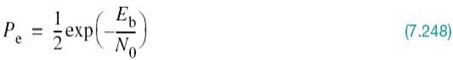
According to this formula, DPSK provides a gain of 3 dB over binary FSK using noncoherent detection for the same E_b/N₀.

Generation of DPSK Signal

Figure 7.44 shows the block diagram of the DPSK transmitter. To be specific, the transmitter consists of two functional blocks:

• Logic network and one-bit delay (storage) element, which are interconnected so as to convert the raw input binary sequence {b_k} into the differentially encoded sequence {d_k}.
• Binary PSK modulator, the output of which is the desired DPSK signal.

Optimum Receiver for the Detection of DPSK

In the use of DPSK, the carrier phase θ is unknown, which complicates the received signal x(t). To deal with the unknown phase θ in the differentially coherent detection of the DPSK signal in x(t), we equip the receiver with an in-phase and a quadrature path. We thus have a signal-space diagram where the received signal points over the two-bit interval are defined by (A cosθ, A sinθ) and (–A cosθ, –A sinθ), where A denotes the carrier amplitude.

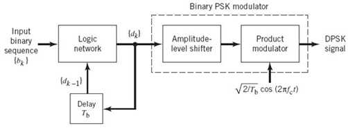
Figure 7.44 Block diagram of a DPSK transmitter.

This geometry of possible signals is illustrated in Figure 7.45. For the two-bit interval , the receiver measures the coordinates x_I0, x_Q0 first, at time t = T_b and then measures x_I1, x_Q1 at time t = 2T_b. The issue to be resolved is whether these two points map to the same signal point or different ones. Recognizing that the vectors x₀ and x₁, with end points x_I0, x_Q0 and x_I1, x_Q1, respectively, are points roughly in the same direction if their inner product is positive, we may formulate the binary-hypothesis test with a question:

Is the inner x₀^T x¹ product positive or negative?

Expressing this statement in analytic terms, we may write

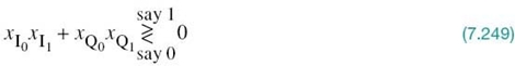
where the threshold is zero for equiprobable symbols.

We now note the following identity:

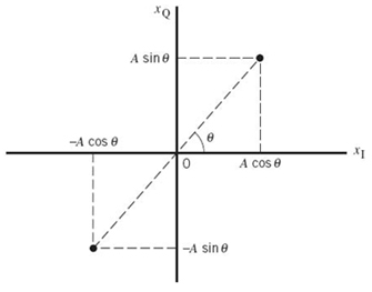
Figure 7.45 Signal-space diagram of received DPSK signal.

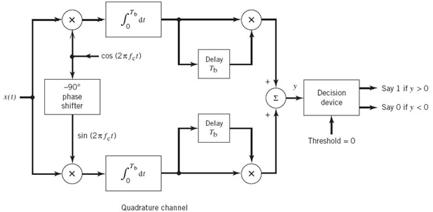
Figure 7.46 Block diagram of a DPSK receiver.

Hence, substituting this identity into (7.249), we get the equivalent test:

where the scaling factor 1/4 is ignored. In light of this equation, the question on the binary hypothesis test for the detection of DPSK may now be restated as follows:

Given the current signal point (x_I0, x_Q0) received in the time interval 0 < t < 2T_b, is this point closer to the signal point (x_I1 , x_Q1) or its image (-x_I1, -x_Q1) received in the next time interval T_b < t < 2T_b?

Thus, the optimum receiver¹¹ for the detection of binary DPSK is as shown in Figure 7.46, the formulation of which follows directly from the binary hypothesis test of (7.250). This implementation is simple, in that it merely requires that sample values be stored.

The receiver of Figure 7.46 is said to be optimum for two reasons:

1.  In structural terms, the receiver avoids the use of fancy delay lines that could be needed otherwise.

2.  In operational terms, the receiver makes the decoding analysis straightforward to handle, in that the two signals to be considered are orthogonal over the interval [0, 2T_b] in accordance with the formula of (7.227).

7.14  BER Comparison of Signaling Schemes over AWGN Channels

Much of the material covered in this chapter has been devoted to digital modulation schemes operating over AWGN channels. In this section, we present a summary of the BERs of some popular digital modulation schemes, classified into two categories, depending on the method of detection used in the receiver:

Class I: Coherent detection

• binary PSK: two symbols, single carrier
• binary FSK: two symbols, two carriers one for each symbol
• QPSK: four symbols, single carrier—the QPSK also includes the QAM, employing four symbols as a special case
• MSK: four symbols, two carriers.

Class II: Noncoherent detection

• DPSK: two symbols, single carrier
• binary FSK: two symbols, two carriers.

Table 7.7 presents a summary of the formulas of the BERs of these schemes separated under Classes I and II. All the formulas are defined in terms of the ratio of energy per bit to the noise spectral density, E_b/N₀, as summarized herein:

1.  Under Class I, the formulas are expressed in terms of the Q-function. This function is defined as the area under the tail end of the standard Gaussian distribution with zero mean and unit variance; the lower limit in the integral defining the Q-function is dependent solely on E_b/N₀, scaled by the factor 2 for binary PSK, QPSK, and MSK. Naturally, as this SNR ratio is increased, the area under the Q-function is reduced and with it the BER is correspondingly reduced

2.  Under Class II, the formulas are expressed in terms of an exponential function, where the negative exponent depends on the E_b/N₀ ratio for DPSK and its scaled version by the factor 1/2 for binary FSK. Here again, as the E_b/N₀ is increased, the BER is correspondingly reduced.

The performance curves of the digital modulation schemes listed in Table 7.7 are shown in Figure 7.47 where the BER is plotted versus E_b/N₀. As expected, the BERs for all the

Table 7.7 Formulas for the BER of digital modulation schemes employing two or four symbols

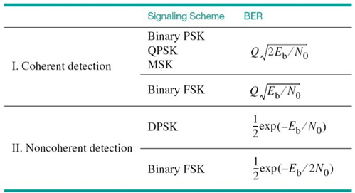
schemes decrease monotonically with increasing E_b/N₀, with all the graphs having a similar shape in the form of a waterfall. Moreover, we can make the following observations from Figure 7.47:

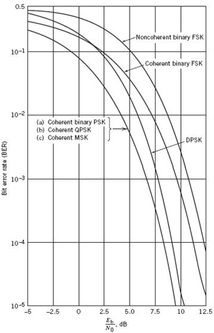
Figure 7.47 Comparison of the noise performance of different PSK and FSK schemes.

1.  For any value of E_b/N₀, the schemes using coherent detection produce a smaller BER than those using noncoherent detection, which is intuitively satisfying.

2.   PSK schemes employing two symbols, namely binary PSK with coherent detection and DPSK with noncoherent detection, require an E_b/N₀ that is 3 dB less than their FSK counterpart to realize the same BER.

3.  At high values of E_b/N₀, DPSK and binary FSK using noncoherent detection perform almost as well, to within about 1 dB of their respective counterparts using coherent detection for the same BER.

4.  Although under Class I the BER for binary PSK, QPSK, and MSK is governed by the same formula, there are important differences between them:

• For the same channel bandwidth and BER, the QPSK accommodates the transmission of binary data at twice the rate attainable with binary PSK; in other words, QPSK is bandwidth conserving.
• When sensitivity to interfering signals is an issue of practical concern, as in wireless communications, MSK is preferred over QPSK.

7.15  Synchronization

The coherent reception of a digitally modulated signal, discussed in previous sections of this chapter, requires that the receiver be synchronous with the transmitter. In this context, we define the process of synchronization as follows:

Two sequences of related events performed separately, one in the transmitter and the other in the receiver, are said to be synchronous relative to each other when the events in one sequence and the corresponding events in the other occur simultaneously, except for some finite delay.

There are two basic modes of synchronization:

1.  Carrier synchronization. When coherent detection is used in signaling over AWGN channels via the modulation of a sinusoidal carrier, knowledge of both the frequency and phase of the carrier is necessary. The process of estimating the carrier phase and frequency is called carrier recovery or carrier synchronization; in what follows, both terminologies are used interchangeably.

2. To perform demodulation, the receiver has to know the instants of time at which the modulation in the transmitter changes its state. That is, the receiver has to know the starting and finishing times of the individual symbols, so that it may determine when to sample and when to quench the product-integrators. The estimation of these times is called clock recovery or symbol synchronization; here again, both terminologies are used interchangeably.

We may classify synchronization schemes as follows, depending on whether some form of aiding is used or not:

1.  Data-aided synchronization. In data-aided synchronization schemes, a preamble is transmitted along with the data-bearing signal in a time-multiplexed manner on a periodic basis. The preamble contains information about the symbol timing, which is extracted by appropriate processing of the channel output at the receiver. Such an approach is commonly used in digital satellite and wireless communications, where the motivation is to minimize the time required to synchronize the receiver to the transmitter. Limitations of data-aided synchronization are twofold:

• reduced data-throughput efficiency, which is incurred by assigning a certain portion of each transmitted frame to the preamble, and
• reduced power efficiency, which results from the allocation of a certain fraction of the transmitted power to the transmission of the preamble.

2.  Nondata-aided synchronization. In this second approach, the use of a preamble is avoided and the receiver has the task of establishing synchronization by extracting the necessary information from the noisy distorted modulated signal at the channel output. Both throughput and power efficiency are thereby improved, but at the expense of an increase in the time taken to establish synchronization.

In this section, the discussion is focused on nondata-aided forms of carrier and clock recovery schemes. To be more specific, we adopt an algorithmic approach,¹² which is so-called on account of the fact that implementation of the sychronizer enables the receiver to estimate the carrier phase and symbol timing in a recursive manner from one time instant to another. The processing is performed on the baseband version of the received signal, using discrete-time (digital) signal-processing algorithms.

Algorithmic Approach to Synchronization

Maximum likelihood decoding played a key role in much of the material on signaling techniques in AWGN channels presented in Sections 7.4 through 7.13. Maximum likelihood parameter estimation plays a key role of its own in the algorithmic approach to synchronization. Both of these methods were discussed previously in Chapter 3 on probability theory and Bayesian inference. In this context, it may therefore be said that a sense of continuity is being maintained throughout this chapter.

Given the received signal, the maximum likelihood method is used to estimate two parameters: carrier phase and symbol timing, both of which are, of course, unknown. Here, we are assuming that knowledge of the carrier frequency is available at the receiver.

Moreover, in the algorithmic approach, the symbol-timing recovery is performed before phase recovery. The rationale for proceeding in this way is that once we know theenvelope delay incurred by signal transmission through a dispersive channel, then one sample per symbol at the matched filter output may be sufficient for estimating the unknown carrier phase. Moreover, computational complexity of the receiver is minimized by using synchronization algorithms that operate at the symbol rate 1/T.

In light of the remarks just made, we will develop the algorithmic approach to synchronization by proceeding as follows:

1.  Through processing the received signal corrupted by channel noise and channel dispersion, the likelihood function is formulated.

2.  The likelihood function is maximized to recover the clock.

3.  With clock recovery achieved, the next step is to maximize the likelihood function to recover the carrier.

The derivations presented in this chapter focus on the QPSK signal. The resulting formulas may be readily extended to binary PSK symbols as a special case and generalized for M-ary PSK signals.

7.16  Recursive Maximum Likelihood Estimation for Synchronization

In the previous section, we remarked that, in algorithmic synchronization, estimation of the two unknown parameters, namely carrier phase and symbol timing, is performed in a recursive manner from one time instant to another.

In other words:

Discrete time is an essential dimension of recursive parameter estimation.

Moreover, the estimation is performed at time t = nT, where n is an integer and T is the symbol duration. Equivalently, we may say that n = t/T denotes the normalized (dimensionless) discrete time.

One other important point to note: recursive estimation of the unknown parameter, be that the carrier phase or symbol time, plays a key role in the synchronization process. Specifically, it proceeds across discrete time in accordance with the following rule:

In other words, the recursive parameter estimation takes on the structure of an adaptive filtering algorithm, in which the product of the step-size parameter and error signal assumes the role of an algorithmic adjustment.

In what follows, we derive adaptive filtering algorithms for estimating the unknown synchronization parameters with the error signal being derived from the likelihood function.

Likelihood Functions

The idea of maximum likelihood parameter estimation based on continuous-time waveforms was discussed in Chapter 3. To briefly review the material described therein, consider a baseband signal defined by

where λ is an unknown parameter and w(t) denotes an AWGN. Given a sample of the signal x(t), the requirement is to estimate the parameter λ; so, we say:

The most likely value of the estimate λ̂ is the particular λ for which the likelihood function l(λ) is a maximum.

Note that we say “a maximum” rather than “the maximum” because it is possible for the graph of l(λ) plotted versus to have multiple maxima. In any event, the likelihood function given x, namely l(λ), is defined as the probability density function f(x∣λ) with the roles of x and λ interchanged, as shown by

where, for convenience of presentation, we have omitted the conditional dependence of λ on x in l(λ).

In the algorithmic synchronization procedures derived in this section, we will be concerned only with cases in which the parameter λ is a scalar. Such cases are referred to as independent estimation. However, when we are confronted with the synchronization of a digital communication receiver to its transmitter operating over a dispersive channel, we have two unknown channel-related parameters to deal with: the phase (carrier) delay τ_g, and the group (envelope) delay τ_c, both of which were discussed in Chapter 2. In the context of these two parameters, when we speak of independent estimation for synchronization, we mean that the two parameters τ_c and τ_g are considered individually rather than jointly. Intuitively speaking, independent estimation is much easier to tackle and visualize than joint estimation, and it may yield more robust estimates in general.

Let the transmitted signal for symbol i in the QPSK signal be defined by

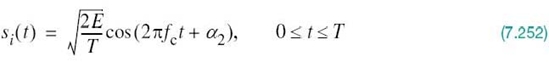
where E is the signal energy per symbol, T is the symbol period, and α_i is the carrier phase used for transmitting symbol i. For example, for the QPSK we have

Equivalently, we may write

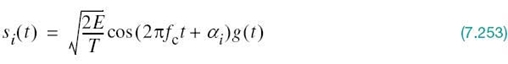
where g(t) is the shaping pulse, namely a rectangular pulse of unit amplitude and duration T. By definition, τ_c affects the carrier and τ_g affects the envelope. Accordingly, the received signal at the channel output is given by

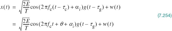
where w(t) is the channel noise. The new term θ introduced in (7.254) is an additive carrier phase attributed to the phase delay τ_c produced by the dispersive channel; it is defined by

The minus sign is included in the right-hand side of (7.255) to be consistent with previous notation used in dealing with signal detection.

Both the carrier phase θ and group delay τ_g are unknown. However, it is assumed that they remain essentially constant over the observation interval 0 ≤ t ≤ T₀ or through the transmission of a sequence made up of L₀ = T₀/T symbols.

With θ used to account for the carrier delay τ_c, we may simplify matters by using τ in place of τ_g for the group delay; that is, (7.254) is rewritten as

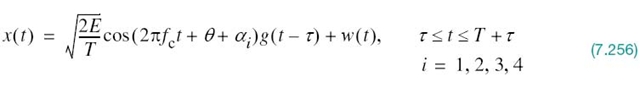
At the receiver, the orthogonal pair of basis functions for QPSK signals is defined by

Here, it is assumed that the receiver has perfect knowledge of the carrier frequency f_c, which is a reasonable assumption; otherwise, a carrier-frequency offset has to be included that will complicate the analysis.

Accordingly, we may represent the received signal x(t) by the baseband vector

where

In a corresponding fashion, we may express the signal component of x(τ) by the vector

where

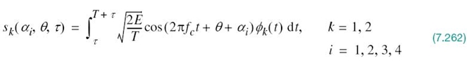
Assuming that f_c is an integer multiple of the symbol rate 1/T, evaluation of the integral in (7.262) shows that dependence of s₁ and s₂ on the group delay τ is eliminated, as shown by

We may thus expand on (7.259) to write

where

The two elements of the noise vector w are themselves defined by

The w_k in (7.267) is the sample value of a Gaussian random variable W of zero mean and variance N₀/2, where N₀/2 is the power spectral density of the channel noise w(t). Dependence of the baseband signal vector x on delay τ is inherited from (7.265).

The conditional probability density function of the random vector X, represented by the sample x at the receiver input given transmission of the ith symbol, and occurrence of the carrier phase θ and group delay τ resulting from the dispersive channel, is defined by

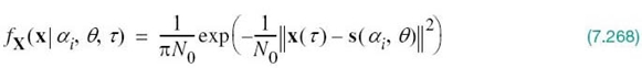
Setting s(α_i, σ) equal to zero, (7.268) reduces to

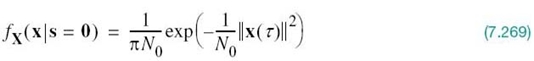
Equation (7.268) defines the probability density function of the random vector X in the combined presence of signal and channel noise, whereas (7.269) defines the probability density function of x in the presence of channel noise acting alone. Accordingly, we may define the likelihood function for QPSK as the ratio of these two probability density functions, as shown by

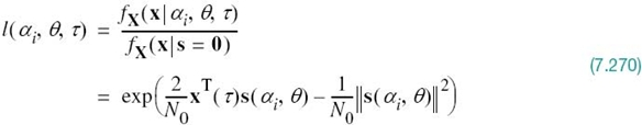
In QPSK, we have

because all four message points lie on a circle of radius . Hence, ignoring the second term in the exponent in (7.270), we may reduce the likelihood function to

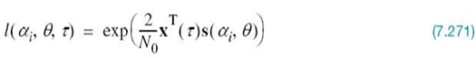
Complex Terminology for Algorithmic Synchronization

Before proceeding with the derivations of adaptive filtering algorithms for recovery of the clock and carrier, we find it instructive to reformulate the likelihood function of (7.271) using complex terminology. Such a step is apropos given the fact that the received signal vector as well as its contituent signal and noise vectors in (7.265) are all in their respective baseband forms.

Specifically, the two-dimensional vector x(τ) is represented by the complex envelope of the received signal

where .

Correspondingly, the signal vector s(α_i, θ), comprising the pair of signal components s₁(α_i, θ) and s₂(α_i, θ), is represented by the complex envelope of the transmitter signal corrupted by carrier phase θ:

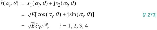
The new complex parameter α̃_i in (7.273) is a symbol indicator in the message constellation of the QPSK; it is defined by

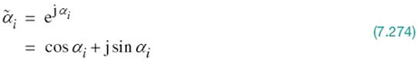
Correspondingly, the complex experimental factor embodying the carrier phase θ is defined by

Both (7.274) and (7.275) follow from Euler’s formula.

With the complex representations of (7.272) to (7.275) at hand, we may now reformulate the exponent of the likelihood function in (7.271) in the equivalent complex form:

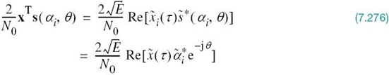
where Re[.] denotes the real part of the complex expression inside the square brackets. Hence, we may make the following statement:

The inner product of the two complex vectors x(τ) and s(α_i, θ) in (7.276) is replaced by times the real part of the inner product of two complex variables: and .

Two points are noteworthy here:

1.  The complex envelope of the received signal is dependent on the group delay τ, hence . The product is made up of the complex symbol indicator attributed to the QPSK signal generated in the transmitter and the exponential term e^jθ attributed to phase distortion in the channel.

2.  In complex variable theory, given a pair of complex terms and , their inner product could be defined as , as shown in (7.276).

The complex representation on the right-hand side of (7.276), expressed in Cartesian form, is well suited for estimating the unknown phase θ. On the other hand, for estimating the unknown group delay τ, we find it more convenient to use a polar representatio n for the inner product of the two vectors x(τ) and s(α_i, θ), as shown by

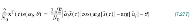
Indeed, it is a straightforward matter to show that the two complex representations on the right-hand side of (7.276) and (7.277) are indeed equivalent. The reasons for why these two representations befit the estimation of carrier phase θ and group delay τ, respectively, will become apparent in the next two subsections.

Moreover, in light of what was said previously, estimation of the group delay should precede that of the carrier phase. Accordingly, the next subsection is devoted to group-delay estimation, followed by the sub-section devoted to carrier-phase estimation.

Recursive Estimation of the Group Delay

To begin the task of estimating the unknown group delay, first of all we have to remove dependence of the likelihood function l(α_i, σ, τ) on the unknown carrier phase θ in (7.271). To do this, we will average the likelihood function over all possible values of θ inside the range [0, 2π]. To this end, θ is assumed to be uniformly distributed inside this range, as shown by

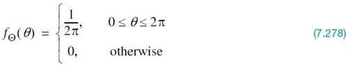
which is the worst possible situation that can arise in practice. Under this assumption, we may thus express the average likelihood function as

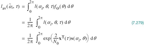
where, in the last line, we used (7.271).

Examining the two alternative complex representations of the likelihood function’s exponent given in (7.276) and (7.277), it is the latter that best suits solving the integration in (7.279). Specifically, we may write

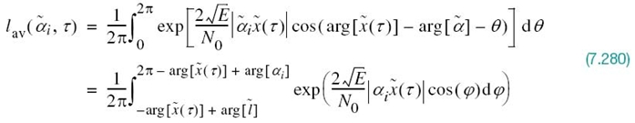
where, in the last line, we have made the substitution

We now invoke the definition of the modified Bessel function of zero order, as shown by (see Appendix C)

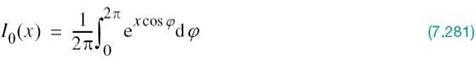
Using this formula, we may, therefore, express the average likelihood function in (7.280) as follows:

where is the complex envelope of the matched filter output in the receiver. By definition, for QPSK we have

It follows, therefore, that (7.282) reduces to

Here, it is important to note that, as a result of averaging the likelihood function over the carrier phase θ, we have also removed dependence on the transmitted symbol for QPSK; this result is intuitively satisfying.

In any event, taking the natural logarithm of l_av(τ) in (7.283) to obtain the log-likelihood function of τ, we write

where ln denotes the natural logarithm. To proceed further, we need to find a good approximation for L_av(τ). To this end, we first note that the modified Bessel function I₀(x) may itself be expanded in a power series (see Appendix C):

where x stands for the product term . For small values of x, we may thus approximate I₀(x) as shown by

We may further simplify matters by using the approximation

For the problem at hand, small x corresponds to small SNR. Under this condition, we may now approximate the log-likelihood function of (7.284) as follows:

With maximization of L_av(τ) as the objective, we differentiate it with respect to the envelope delay τ, obtaining

where is the complex conjugate of and is its derivative with respect to τ.

The formula in (7.287) is the result of operating on the received signal at the channel output, x(t), defined in (7.254) for a particular symbol of the QPSK signal defined in the interval [τ, T + τ]. In the course of finding the baseband vector representation of the received signal, namely x̃(τ), dependence on time t disappeared in (7.287). Notwithstanding this point, the fact of the matter is the log-likelihood ratio M_av(τ) in (7.287) pertains to some point in discrete time n = t/T, and it changes with n. To go forward with recursive estimation of the group delay τ, we must therefore bring discrete time n into the procedure. To this end, n is assigned as a subscript to both and x'̃(τ) in (7.287). Thus, with the recursive estimation of following the format described in words in (7.251), we may define the error signal needed for the recursive estimation of τ (i.e., symbol-timing recovery) as follows:

Let τ ̂_n denote the estimate of the unknown group delay τ at discrete time n. Correspondingly, we may introduce two definitions

and

Accordingly, we may reformulate the error signal e_n in (7.288) as follows:

Computation of the error signal e_n, therefore, requires the use of two filters:

1.  Complex matched filter, which is used for generating .

2.  Complex derivative matched filter, which is used for generating .

By design, the receiver is already equipped with the first filter. The second one is new. In practice, the additional computational complexity due to the derivative matched filter is found to be an undesireable requirement. To dispense with the need for it, we propose to approximate the derivative using a finite difference, as shown by

Note, however, that in using the finite-difference approximation of (7.292) we have simplified computation of the derivative matched filter by doubling the symbol rate. It is desirable to make one further modification to account for the fact that timing estimates are updated at multiples of the symbol period T and the only available quantities are τ̂_n. Consequently, we replace τ̂_n+1/2 by the current (updated estimate) τ̂_n and replace τ̂_n–1/2 by the old estimate τ̂_n–1. We may thus rewrite (7.292) as follows:

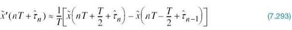
So, we finally redefine the error signal as follows:

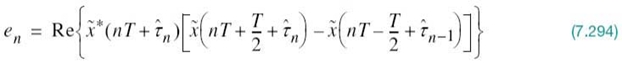
where the scaling factor 1/T is accounted for in what follows.

Finally, building on the format of the recursive estimation procedure described in (7.251), we may formulate the adaptive filtering algorithm for symbol timing recovery:

where we have the following:

• The γ in (7.295) is the step-size parameter, in which the two scaling factors 2E/N²₀ and 1/T are absorbed; the factor 2E/N²₀ was ignored in moving from (7.287) to (7.288) and the factor 1/T was ignored from (7.293) to (7.294).
• The error signal e_n is defined by (7.294).
• The c_n is a real number employed as control for the frequency of an oscillator, referred to as a number-controlled oscillator (NCO).

The closed-loop feedback system for implementing the timing-recovery algorithm of (7.295) is shown in Figure 7.48. From a historical perspective, the scheme shown in this figure is analogous to the continuous-time version of the traditional early–late gate synchronizer widely used for timing recovery. In light of this analogy, the scheme of Figure 7.48 is referred to as a recursive early–late delay (NDA-ELD) synchronizer. At every recursion (i.e., time step), the synchronizer works on three successive samples of the matched filter output, namely:

The first sample is early and the last one is late, both defined with respect to the middle one.

Recursive Estimation of the Carrier Phase

With estimation of the symbol time τ taken care of, the next step is to estimate the carrier phase θ. This estimation is also based on the likelihood function defined in (7.270), but with a difference: this time we use the complex representation on the right-hand side of (7.276) for the likelihood function’s exponent. Thus, the likelihood function of θ is now expressed as follows:

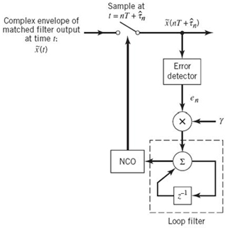
Figure 7.48 Nondata-aided early–late delay synchronizer for estimating the group delay.

Taking the natural logorithm of both sides of (7.296), the log-likelihood function of θ is, therefore, given by

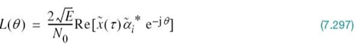
Here again, maximizing the estimate of the carrier phase θ as the issue of interest, we differentiate L(θ) with respect to θ, obtaining

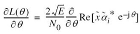
The real-part operator Re[.] is linear; therefore, we may interchange this operation with the differentiation. Moreover, we have

As a result of the differentiation, the argument in (7.297) is multiplied by –j, which, in turn, has the effect of replacing the real-part operator Re[.] by the corresponding imaginary-part operator Im[.] Accordingly, we may express derivative of the log-likelihood function in (7.297) with respect to θ as follows:

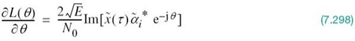
With this equation at hand, we are now ready to formulate the adaptive filtering algorithm for estimating the unknown carrier phase θ. To this end, we incorporate discrete-time n into the recursive estimation procedure for clock recovery in a manner similar to what we did for the group delay; specifically:

1.  With the argument of the imaginary-part operator in (7.298) playing the role of error signal, we write:

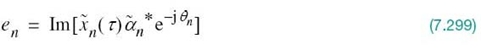
where n denotes the normalized discrete-time.

2.  The scaling factor is absorbed in the new step-size parameter μ.

3.  With denoting the old estimate of the carrier phase θ and denoting its updated value, the update rule for the estimation is defined as follows:

Equations (7.299) and (7.300) not only define the adaptive filtering algorithm for carrier-phase estimation, but also they provide the basis for implementing the algorithm, as shown in Figure 7.49. This figure may be viewed as a generalization of the well-known Costas loop for the analog synchronization of linear quadrature-amplitude modulation schemes that involve the combined use of in-phase and quadrature components, of which the QPSK is a special example. As such, we may refer to the closed-loop synchronization scheme of Figure 7.49 as the recursive Costas loop for phase synchronization.

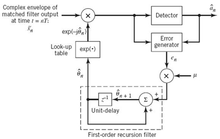
Figure 7.49 The recursive Costas loop for estimating the carrier phase.

The following points should be noted in Figure 7.49:

• The detector supplies an estimate of the symbol indicator α̂_n and, therefore, the transmitted symbol, given the matched filter output.
• For the input , the look-up table in the figure supplies the value of the exponential

  

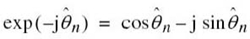
• The output of the error generator is the error signal e_n, defined in (7.299).
• The block labeled z^–1 represents a unit-time delay.

The recursive Costas loop of Figure 7.49 uses a first-order digital filter. To improve the tracking performance of this synchronization system, we may use a second-order digital filter. Figure 7.50 shows an example of a second-order recursive filter made up of a cascade of two first-order sections, with ρ as an adjustable loop parameter. An important property of a second-order recursive filter used in the Costas loop for phase recovery is that it will eventually lock onto the incoming carrier with no static error, provided that the frequency error between the receiver and transmitter is initially small.

Convergence Considerations

The adaptive behavior of the filtering schemes in Figures 7.48 and 7.49 for group-delay and carrier-phase estimation, respectively, is governed by how the step-size parameters γ are μ selected. The smaller we make γ and, likewise, μ, the more refined will be the trajectories resulting from application of the algorithms. However, this benefit is attained at the cost of the number of recursions required for convergence of the algorithms. On the other hand, if the step-size parameter γ and μ is assigned a large value, then the trajectories may follow a zig-zag sort of path. Indeed, if γ and μ exceeds a certain critical value of its own, it is quite possible for the algorithm to diverge, which means that the synchronization schemes of Figures 7.48 and 7.49 may become unstable. So, from a design perspective, the compromise choice between accuracy of estimation and speed of convergence may require a detailed attention, both theoretical and experimental.

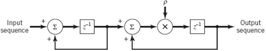
Figure 7.50 Second-order recursive filter.

7.17  Summary and Discussion

The primary goal of the material presented in this chapter is the formulation of a systematic procedure for the analysis and design of a digital communication receiver in the presence of AWGN. The procedure, known as maximum likelihood detection, decides which particular transmitted symbol is the most likely cause of the noisy signal observed at the channel output. The approach that led to the formulation of the maximum likelihood detector (receiver) is called signal-space analysis. The basic idea of the approach is to represent each member of a set of transmitted signals by an N-dimensional vector, where N is the number of orthonormal basis functions needed for a unique geometric representation of the transmitted signals. The set of signal vectors so formed defines a signal constellation in an N-dimensional signal space.

For a given signal constellation, the (average) probability of symbol error, P_e, incurred in maximum likelihood signal detection over an AWGN channel is invariant to rotation of the signal constellation as well as its translation. However, except for a few simple (but important) cases, the numerical calculation of P_e is an impractical proposition. To overcome this difficulty, the customary practice is to resort to the use of bounds that lend themselves to computation in a straightforward manner. In this context, we described the union bound that follows directly from the signal-space diagram. The union bound is based on an intuitively satisfying idea:

The probability of symbol error P_e is dominated by the nearest neighbors to the transmitted signal in the signal-space diagram.

The results obtained using the union bound are usually fairly accurate, particularly when the SNR is high.

With the basic background theory on optimum receivers covered in the early part of Chapter 7 at our disposal, formulas were derived for, or bounds on, the BER for some important digital modulation techniques in an AWGN channel:

1.  PSK, using coherent detection; it is represented by

• binary PSK;
• QPSK and its variants, namely, such as the offset QPSK;
• coherent M-ary PSK, which includes binary PSK and QPSK as special cases with M = 2 and M = 4, respectively.

The DPSK may be viewed as the pseudo-noncoherent form of PSK.

2.  M-ary QAM, using coherent detection; this modulation scheme is a hybrid form of modulation that combines amplitude and phase-shift keying. For M = 4, it includes QPSK as a special case.

3.  FSK, using coherent detection; it is represented by

• binary FSK;
• MSK and its Gaussian variant known as GMSK;
• M-ary FSK.

4.  Noncoherent detection schemes, involving the use of binary FSK and DPSK.

Irrespective of the digital modulation system of interest, synchronization of the receiver to the transmitter is essential to the operation of the system. Symbol timing recovery is required whether the receiver is coherent or not. If the receiver is coherent, we also require provision for carrier recovery. In the latter part of the chapter we discussed nondata-aided synchronizers to cater to these two requirements with emphasis on M-ary PSK, exemplified by QPSK signals, in which the carrier is suppressed. The presentation focused on recursive synchronization techniques that are naturally suited for the use of discrete-time signal processing algorithms.

We conclude the discussion with some additional notes on the two adaptive filtering algorithms described in Section 7.16 on estimating the unknown parameters: carrier phase and group delay. In a computational context, these two algorithms are in the same class as the celebrated least-mean-square (LMS) algorithm described by Widrow and Hoff over 50 years ago. The LMS algorithm is known for its computational efficiency, effectiveness in performance, and robustness with respect to the nonstationary character of the environment in which it is embedded. The two algorithmic phase and delay synchronizers share the first two properties of the LMS algorithm; for a conjecture, it may well be they are also robust when operating in a nonstationary communication environment.

   Problems

     Representation of Signals

7.1   In Chapter 6 we described line codes for pulse-code modulation. Referring to the material presented therein, formulate the signal constellations for the following line codes:

a. unipolar nonreturn-to-zero code

b. polar nonreturn-to-zero code

c. unipolar return-to-zero code

d. manchester code.

7.2   An 8-level PAM signal is defined by

where A_i = ±1, ±3, ±5, ±7. Formulate the signal constellation of .

7.3    Figure P7.3 displays the waveforms of four signals s₁(t), s₂(t), s₃(t), and s₄(t).

a. Using the Gram–Schmidt orthogonalization procedure, find an orthonormal basis for this set of signals.

b. Construct the corresponding signal-space diagram.

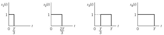
Figure P7.3

7.4   a. Using the Gram–Schmidt orthogonalization procedure, find a set of orthonormal basis functions to represent the three signals s₁(t), s₂(t), and s₃(t) shown in Figure P7.4.

b. Express each of these signals in terms of the set of basis functions found in part a.

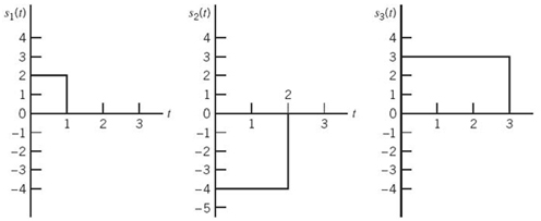
Figure P7.4

7.5   An orthogonal set of signals is characterized by the property that the inner product of any pair of signals in the set is zero. Figure P7.5 shows a pair of signals s₁(t) and s₂(t) that satisfy this definition. Construct the signal constellation for this pair of signals.

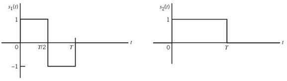
Figure P7.5

7.6  A source of information emits a set of symbols denoted by . Two candidate modulation schemes, namely pulse-duration modulation (PDM) and pulse-position modulation (PPM), are considered for the electrical representation of this set of symbols. In PDM, the ith symbol is represented by a pulse of unit amplitude and duration (i/M)T. On the other hand, in PPM, the ith symbol is represented by a short pulse of unit amplitude and fixed duration, which is transmitted at time t = (i/M)T. Show that PPM is the only one of the two that can produce an orthogonal set of signals over the interval 0 ≤ t ≤ T.

7.7  A set of 2M biorthogonal signals is obtained from a set of M ordinary orthogonal signals by augmenting it with the negative of each signal in the set.

a. The extension of orthogonal to biorthogonal signals leaves the dimensionality of the signal space unchanged. Explain how.

b. Construct the signal constellation for the biorthogonal signals corresponding to the pair of orthogonal signals shown in Figure P7.5.

7.8   a. A pair of signals s_i(t) and s_k(t) have a common duration T. Show that the inner product of this pair of signals is given by

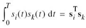
where s_i and s_k are the vector representations of s_i(t) and s_k(t), respectively.

b. As a follow-up to part a of the problem, show that

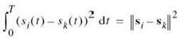
7.9  Consider a pair of complex-valued signals s_i(t) and s_k(t) that are respectively represented by

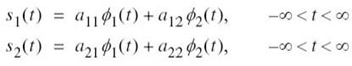
where the basis functions ϕ₁(t) and ϕ₂(t) are both real valued, but the coefficients a₁₁, a₁₂, a₂₁, and a₂₂ are complex valued. Prove the complex form of the Schwarz inequality:

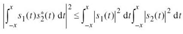
where the asterisk denotes complex conjugation. When is this relation satisfied with the equality sign?

Stochastic Processes

7.10  Consider a stochastic process X(t) expanded in the form

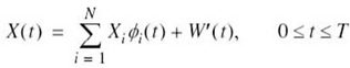
where W'(t) is a remainder noise term. The form an orthonormal set over the interval 0 ≤ t ≤ T, and the random variable X_i is defined by

Let W′(t_k) denote a random variable obtained by observing W′(t) at time t = t_k. Show that

7.11  Consider the optimum detection of the sinusoidal signal in AWGN:

a. Determine the correlator output assuming a noiseless input.

b. Determine the corresponding matched filter output, assuming that the filter includes a delay T to make it causal.

c. Hence, show that these two outputs are exactly the same only at the time instant t = T.

Probability of Error

7.12  Figure P7.12 shows a pair of signals s₁(t) and s₂(t) that are orthogonal to each other over the observation interval 0 ≤ t ≤ 3T. The received signal is defined by

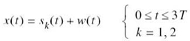
where w(t) is white Gaussian noise of zero mean and power spectral density N₀/2.

a. Design a receiver that decides in favor of signals s₁(t) or s₂(t), assuming that these two signals are equiprobable.

b. Calculate the average probability of symbol error incurred by this receiver for E/N₀ = 4, where E is the signal energy.

Figure P7.12

7.13  In the Manchester code discussed in Chapter 6, binary symbol 1 is represented by the doublet pulse s(t) shown in Figure P7.13, and binary symbol 0 is represented by the negative of this pulse. Derive the formula for the probability of error incurred by the maximum likelihood detection procedure applied to this form of signaling over an AWGN channel.

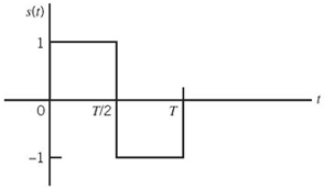
Figure P7.13

7.14  In the Bayes’ test, applied to a binary hypothesis-testing problem where we have to choose one of two possible hypotheses H₀ and H₁, we minimize the risk defined by

The parameters C₀₀, C₁₀, C₁₁, and C₀₁ denote the costs assigned to the four possible outcomes of the experiment: the first subscript indicates the hypothesis chosen and the second the hypothesis that is true. Assume that C₁₀ > C₀₀ and C₀₁ > C₁₁. The p₀ and p₁ denote the a priori probabilities of hypotheses H₀ and H₁, respectively.

a. Given the observation vector x, show that the partitioning of the observation space so as to minimize the risk leads to the likelihood ratio test:

where Λ(x) is the likelihood ratio defined by

and λ is the threshold of the test defined by

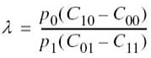
b. What are the cost values for which the Bayes’ criterion reduces to the minimum probability of error criterion?

Principles of Rotational and Translational Invariance

7.15  Continuing with the four line codes considered in Problem 7.1, identify the line codes that have minimum average energy and those that do not. Compare your answers with the observations made on these line codes in Chapter 6.

7.16  Consider the two constellations shown in Figure 7.10. Determine the orthonormal matrix Q that transforms the constellation shown in Figure 7.10a into the one shown in Figure 7.10b.

7.17   a. The two signal constellations shown in Figure P7.17 exhibit the same average probability of symbol error. Justify the validity of this statement.

b. Which of these two constellations has minimum average energy? Justify your answer.

You may assume that the symbols pertaining to the message points displayed in Figure P7.17 are equally likely.

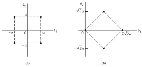
Figure P7.17

7.18  Simplex (transorthogonal) signals are equally likely highly-correlated signals with the most negative correlation that can be achieved with a set of M orthogonal signals. That is, the correlation coefficient between any pair of signals in the set is defined by

One method of constructing simplex signals is to start with a set of M orthogonal signals each with energy E and then apply the minimum energy translate.

Consider a set of three equally likely symbols whose signal constellation consists of the vertices of an equilateral triangle. Show that these three symbols constitute a simplex code.

Amplitude-Shift Keying

7.19  In the on–off keying version of an ASK system, symbol1 is represented by transmitting a sinusoidal carrier of amplitude , where E_b is the signal energy per bit and T_b is the bit duration. Symbol 0 is represented by switching off the carrier. Assume that symbols 1 and 0 occur with equal probability.

For an AWGN channel, determine the average probability of error for this ASK system under the following scenarios:

a. Coherent detection.

b. Noncoherent detection, operating with a large value of bit energy-to-noise spectral density ratio E_b/N₀.

Note: when x is large, the modified Bessel function of the first kind of zero order may be approximated as follows (see AppendixC):

Phase-Shift Keying

7.20  The PSK signal is applied to a correlator supplied with a phase reference that lies within φ radians of the exact carrier phase. Determine the effect of the phase error φ on the average probability of error of the system.

7.21  The signal component of a PSK system scheme using coherent detection is defined by

where 0 ≤ t 2264; T_b, the plus sign corresponds to symbol 1, and the minus sign corresponds to symbol 0; the parameter k lies in the range 0 < k < 1. The first term of s(t) represents a carrier component included for the purpose of synchronizing the receiver to the transmitter.

a. Draw a signal-space diagram for the scheme described here. What observations can you make about this diagram?

b. Show that, in the presence of AWGN of zero mean and power spectral density N₀/2, the average probability of error is

where

c. Suppose that 10% of the transmitted signal power is allocated to the carrier component. Determine the E_b/N₀ required to realize P_e = 10^–4.

d. Compare this value of E_b/N₀ with that required for a binary PSK scheme using coherent detection, with the same probability of error.

7.22   a. Given the input binary sequence 1100100010, sketch the waveforms of the in-phase and quadrature components of a modulated wave obtained using the QPSK based on the signal set of Figure 7.16.

b. Sketch the QPSK waveform itself for the input binary sequence specified in part a.

7.23  Let P_eI and P_eQ denote the probabilities of symbol error for the in-phase and quadrature channels, respectively, of a narrowband digital communication system. Show that the average probability of symbol error for the overall system is given by

7.24  Equation (7.132) is an approximate formula for the average probability of symbol error for M-ary PSK using coherent detection. This formula was derived using the union bound in light of the signal-space diagram of Figure 7.22b. Given that message point m₁ was transmitted, show that the approximation of (7.132) may be derived directly from Figure 7.22b.

7.25  Find the power spectral density of an offset QPSK signal produced by a random binary sequence in which symbols 1 and 0 (represented by ±1) are equally likely and the symbols in different time slots are statistically independent and identically distributed.

7.26  Vestigial sideband modulation (VSB), discussed in Chapter 2, offers another possible modulation method for signaling over an AWGN channel.

a. In particular, a digital VSB transmission system may be viewed as a time-varying one-dimensional system operating at a rate of 2/T dimensions per second, where T is the symbol period. Justify the validity of this statement.

b. Show that digital VSB is indeed equivalent in performance to the offset QPSK.

Quadrature Amplitude Modulation

7.27  Referring back to Example 7, develop a systematic procedure for constructing M-ary QAM constellations given the M-ary QAM constellation of Figure 7.24 for M = 16. In effect, this problem addresses the opposite approach to that described in Example 7.

7.28  Figure p7.28 describes the block diagram of a generalized M-ary QAM modulator. Basically, the modulator includes a mapper that produces a complex amplitude a_m input for m = 0, 1,…,M – 1, The real and imaginary parts of a_m input the basis functions ϕ₁(t) and ϕ₁(t), respectively. The modulator is generalized in that it embodies M-ary PSK and M-ary PAM as special cases.

a. Formulate the underlying mathematics of the modulator described in Figure P7.28

.

b. Hence, show that M-ary PSK and M-ary PAM are indeed special cases of the M-ary QPSK generated by the block diagram of Figure P7.28.

Figure p7.28

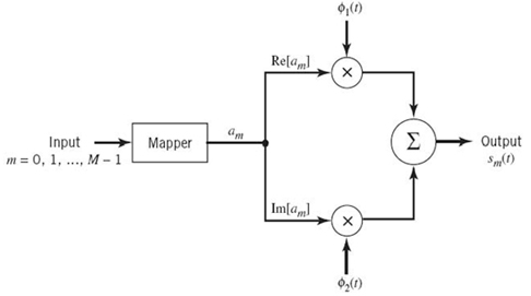
Frequency-Shift Keying

7.29  The signal vectors s₁ and s₂ are used to represent binary symbols 1 and 0, respectively, in a binary FSK system using coherent detection. The receiver decides in favor of symbol1 when

where x^Ts_i is the inner product of the observation vector x and the signal vector s_i, i = 1, 2. Show that this decision rule is equivalent to the condition x₁ > x₂, where x₁ and x₂ are the two elements of the observation vector x. Assume that the signal vectors s₁ and s₂ have equal energy.

7.30  An FSK system transmits binary data at the rate of 2.5 × 10⁶ bits/s. During the course of transmission, white Gaussian noise of zero mean and power spectral density 10^–20 W/Hz is added to the signal. In the absence of noise, the amplitude of the received sinusoidal wave for digit 1 or 0 is 1mV. Determine the average probability of symbol error for the following system configurations:

a. binary FSK using coherent detection;

b. MSK using coherent detection;

c. binary FSK using noncoherent detection.

7.31  In an FSK system using coherent detection, the signals s₁(t) and s₂(t) representing binary symbols 1 and 0, respectively, are defined by

Assuming that f_c > Δf, show that the correlation coefficient of the signals s₁(t) and s₂(t) is approximately given by

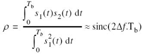
a. What is the minimum value of frequency shift Δf for which the signals s₁(t) and s₂(t) are orthogonal?

b. What is the value of Δf that minimizes the average probability of symbol error

c. For the value of Δf obtained in part c, determine the increase in E_b/N₀ required so that this FSK scheme has the same noise performance as a binary PSK scheme system, also using coherent detection.

7.32  A binary FSK signal with discontinuous phase is defined by

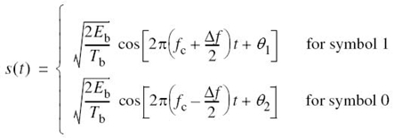
where E_b is the signal energy per bit, T_b is the bit duration, and θ₁ and θ₂ are sample values of uniformly distributed random variables over the interval 0 to 2π. In effect, the two oscillators supplying the transmitted frequencies f_c ± Δf /2 operate independently of each other. Assume that f_c >>Δf.

a. Evaluate the power spectral density of the FSK signal.

b. Show that, for frequencies far removed from the carrier frequency f_c, the power spectral density falls off as the inverse square of frequency. How does this result compare with a binary FSK signal with continuous phase?

7.33  Set up a block diagram for the generation of Sunde’s FSK signal s(t) with continuous phase by using the representation given in (7.170), which is reproduced here

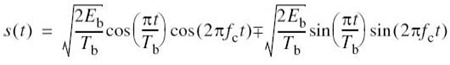
7.34  Discuss the similarities between MSK and offset QPSK, and the features that distinguish them.

7.35  There are two ways of detecting an MSK signal. One way is to use a coherent receiver to take full advantage of the phase information content of the MSK signal. Another way is to use a noncoherent receiver and disregard the phase information. The second method offers the advantage of simplicity of implementation at the expense of a degraded noise performance. By how many decibels do we have to increase the bit energy-to-noise density ratio E_b/N₀ in the second method so as to realize the same average probability of symbol error equal to 10^–5?

7.36   a. Sketch the waveforms of the in-phase and quadrature components of the MSK signal in response to the input binary sequence 1100100010.

b. Sketch the MSK waveform itself for the binary sequence specified in part a.

7.37  An NRZ data stream of amplitude levels ±1 is passed through a low-pass filter whose impulse response is defined by the Gaussian function

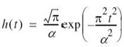
where α is a design parameter defined in terms of the filter’s 3dB bandwidth by

a. Show that the transfer function of the filter is defined by

Hence, demonstrate that the 3dB bandwidth of the filter is indeed equal to W. You may use the list of Fourier-transform pairs in Table 2.1.

b. Determine the response of the filter to a rectangular pulse of unit amplitude and duration T centered on the origin.

7.38  Summarize the similarities and differences between the standard MSK and Gaussian filtered MSK signals.

7.39  Summarize the basic similarities and differences between the standard MSK and QPSK.

Noncoherent Receivers

7.40  In Section 7.12 we derived the formula for the BER of binary FSK using noncoherent detection as a special case of noncoherent orthogonal modulation. In this problem we revisit this issue. As before, we assume that symbol 1 is represented by signal s₁(t) and symbol 0 is represented by signal s₂(t).

According to the material presented in Section 7.12, we note the following:

• The random variable L₂ represented by the sample value l₂ is Rayleigh distributed.
• The random variable L₁ represented by the sample value l₁ is Rician distributed.

The Rayleigh and Rician distributions were discussed in Chapter 4. Using the probability distributions defined in that chapter, derive (7.245) for the BER of binary FSK, using noncoherent detection.

7.41  Figure P7.41a shows a noncoherent receiver using a matched filter for the detection of a sinusoidal signal of known frequency but random phase and under the assumption of AWGN. An alternative implementation of this receiver is its mechanization in the frequency domain as a spectrum analyzer receiver, as in Figure P7.41b, where the correlator computes the finite-time autocorrelation function defined by

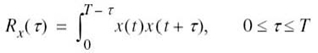
Show that the square-law envelope detector output sampled at time t = T in Figure P7.41a is twice the spectral output of the Fourier transform sampled at frequency f = f_c in Figure P7.41b.

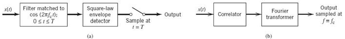
Figure P7.41

7.42  The binary sequence 1100100010 is applied to the DPSK transmitter of Figure 7.44.

a. Sketch the resulting waveform at the transmitter output.

b. Applying this waveform to the DPSK receiver of Figure 7.46, show that in the absence of noise the original binary sequence is reconstructed at the receiver output.

Comparison of Digital Modulation Schemes Using a Single Carrier

7.43  Binary data are transmitted over a microwave link at the rate of 10⁶ bits/s and the power spectral density of the noise at the receiver input is 10^–10 W/Hz. Find the average carrier power required to maintain an average probability of error P_e ≤ 10^–4 for the following schemes:

a. Binary PSK using coherent detection;

a. DPSK.

7.44  The values of E_b/N₀ required to realize an average probability of symbol error P_e = 10^–4 for binary PSK and binary FSK schemes are equal to 7.2 and 13.5, respectively. Using the approximation

determine the separation in the values of E_b/N₀ for P_e = 10^–4, using:

a. binary PSK using coherent detection and DPSK;

b. binary PSK and QPSK, both using coherent detection;

c. binary FSK using (i) coherent detection and (ii) noncoherent detection;

d binary FSK and MSK, both using coherent detection.

7.45  In Section 7.14 we compared the noise performances of various digital modulation schemes under the two classes of coherent and noncoherent detection; therein, we used the BER as the basis of comparison. In this problem we take a different viewpoint and use the average probability of symbol error P_e, to do the comparison. Plot P_e versus E_b/N₀ for each of these schemes and comment on your results.

Synchronization

7.46  Demonstrate the equivalence of the two complex representations given in (7.276) and (7.277), which pertain to the likelihood function.

7.47   a. In the recursive algorithm of (7.295) for symbol timing recovery, the control signals c_n and c_{n + 1} are both dimensionless. Discuss the units in which the error signal e_n and step-size parameter μ are measured.

b. In the recursive algorithm of (7.300) for phase recovery, the old estimate and the updated estimate of the carrier phase θ are both measured in radians. Discuss the units in which the error signal e_n and step-size parameter μ are measured.

7.48 The binary PSK is a special case of QPSK. Using the adaptive filtering algorithms derived in Section 7.16 for estimating the group delay τ and carrier phase θ, find the corresponding adaptive filtering algorithms for binary PSK.

7.49  Repeat Problem 7.48, but this time find the adaptive filtering algorithms for M-ary PSK.

7.50  Suppose we transmit a sequence of L₀ statistically independent symbols of a QPSK signal, as shown by

where L₀ is not to be confused with the symbol for average log-likelihood L_av. The channel output is corrupted by AWGN of zero mean and power spectral density N₀/2, carrier phase θ, and unknown group delay τ.

a. Determine the likelihood function with respect to the group delay τ, assuming that θ is uniformly distributed.

b. Hence, formulate the maximum likelihood estimate of the group delay τ.

c. Compare this feedforward scheme of group-delay estimation with that provided by the NDAELD synchronizer of Figure 7.48.

7.51  Repeat Problem 7.50, but this time do the following:

a. Determine the likelihood function with respect to the carrier phase θ, assuming that the group delay τ is known.

b. Hence, formulate the maximum likelihood estimate of the carrier phase θ.

c. Compare this feedforward scheme of a carrier-phase estimation with the recursive Costas loop of Figure 7.49.

7.52  In Section 7.16 we studied a nondata-aided scheme for carrier phase recovery, based on the log-likelihood function of (7.296). In this problem we explore the use of this equation for data-aided carrier phase recovery.

a. Consider a receiver designed for a linear modulation system. Given that the receiver has knowledge of a preamble of length L₀, show that the maximum likelihood estimate of the carrier phase is defined by

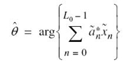
where the preamble is a known sequence of complex symbols and is the complex envelope of the corresponding received signal.

b. Using the result derived in part a, construct a block diagram for the maximum likelihood phase estimator.

7.53   Figure P7.53 shows the block diagram of a phase-synchronization system. Determine the phase estimate of the unknown carrier phase in the received signal x(t).

Figure P7.53

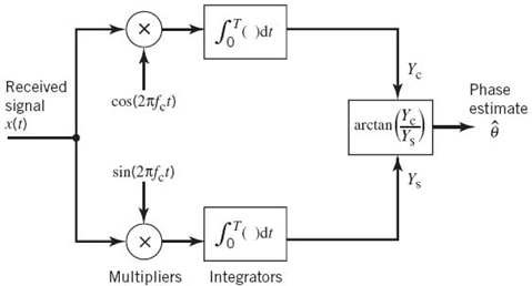
Computer Experiments

**7.54  In this computer-oriented problem, we study the operation of the NDA-ELD synchronizer for symbol timing recovery by considering a coherent QPSK system with the following specifications:

• The channel response is described by a raised cosine pulse with rolloff factor α = 0.5.
• The recursive filter is a first-order digital filter with transfer function

  

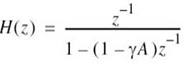
  where z^–1 denotes unit delay, γ is the step-size parameter, and A is a parameter, to be defined.

• The loop bandwidth B_L is 2% of the symbol rate 1/T, that is, B_LT = 0.02.

With symbol timing recovery as the objective, a logical way to proceed is to plot the S-curve for the NDA-ELD under the following conditions:

a. E_b/N₀ = 10 dB

b. E_b/N₀ = ∞(i.e., noiseless channel).

For NDA-ELD, the scheme shown in Figure P7.54 is responsible for generating the S-curve that plots the timing offset versus the discrete time n = t/T.

Using this scheme, plot the S-curves, and comment on the results obtained for parts a and b.

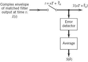
Figure P7.54

7.55  In this follow-up to the computer-oriented Problem 7.54, we study the recursive Costas loop for phase recovery using the same system specifications described in Problem 7.54. This time, however, we use the scheme of Figure P7.54 for measuring the S-curve to plot the phase error versus discrete-time n = t/T.

Figure P7.55

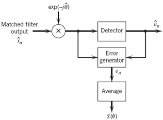
The plot is to be carried out under the following conditions:

a. E_b/N₀ = 5 dB

b. E_b/N₀ = 10 dB

c. E_b/N₀ = 30 dB (i.e., practically noiseless channel)

Comment on the results obtained for these three conditions.

        Notes

1. The geometric representation of signals was first developed by Kotel’nikov (1947) which is a translation of the original doctoral dissertation presented in January 1947 before the Academic Council of the Molotov Energy Institute in Moscow. In particular, see Part II of the book. This method was subsequently brought to fuller fruition in the classic book by Wozencraft and Jacobs (1965).

2. The classic reference for the union bound is Wozencraft and Jacobs (1965).

3. Appendix C addresses the derivation of simple bounds on the Q-function. In (7.88), we have used the following bound:

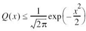
which becomes increasingly tight for large positive values of x.

4. For an early paper on the offset QPSK, see Gitlin and Ho (1975).

5. The MSK signal was first described in Doelz and Heald (1961). For a tutorial review of MSK and comparison with QPSK, see Pasupathy (1979). Since the frequency spacing is only half as much as the conventional spacing of 1/T_b that is used in the coherent detection of binary FSK signals, this signaling scheme is also referred to as fast FSK; see deBuda (1972), who was not aware of the Doelz–Heald patent.

6. For early discussions of GMSK, see Murota and Hirade (1981) and Ishizuke and Hirade (1980).

7. The analytical specification of the power spectral density of digital FM is difficult to handle, except for the case of a rectangular shaped modulating pulse. The paper by Garrison (1975) presents a procedure based on the selection of an appropriate duration-limited/level-quantized approximation for the modulating pulse. The equations developed therein are particularly suitable for machine computation of the power spectra of digital FM signals; see the book by Stüber (1996).

8. A detailed analysis of the spectra of M-ary FSK for an arbitrary value of frequency deviation is presented in the paper by Anderson and Salz (1965).

9. Readers who are not interested in the formal derivation of (7.227) may at this point wish to move on to the treatment of noncoherent binary FSK (in Section 7.12) and DPSK (in Section 7.13), two special cases of noncoherent orthogonal modulation, without loss of continuity.

10. The standard method of deriving the BER for noncoherent binary FSK, presented in McDonough and Whalen (1995) and that for DPSK presented in Arthurs and Dym (1962), involves the use of the Rician distribution. This distribution arises when the envelope of a sine wave plus additive Gaussian noise is of interest; see Chapter 4 for a discussion of the Rician distribution. The derivations presented herein avoid the complications encountered in the standard method.

11. The optimum receiver for differential phase-shift keying is discussed in Simon and Divsalar

12. For detailed treatment of the algorithmic approach for solving the synchronization problem in signaling over AWGN channels, the reader is referred to the books by Mengali and D’Andrea (1997) and Meyer et al. (1998). For books on the traditional approach to synchronization, the reader is referred to Lindsey and Simon (1973).