
CHAPTER
8
Signaling over Band-Limited Channels
8.1 Introduction
In Chapter 7 we focused attention on signaling over a channel that is assumed to be distortionless except for the AWGN at the channel output. In other words, there was no limitation imposed on the channel bandwidth, with the energy per bit to noise spectral density ratio Eb/N0 being the only factor to affect the performance of the receiver. In reality, however, every physical channel is not only noisy, but also limited to some finite bandwidth. Hence the title of this chapter: signaling over band-limited channels.
The important point to note here is that if, for example, a rectangular pulse, representing one bit of information, is applied to the channel input, the shape of the pulse will be distorted at the channel output. Typically, the distorted pulse may consist of a main lobe representing the original bit of information surrounded by a long sequence of sidelobes on each side of the main lobe. The sidelobes represent a new source of channel distortion, referred to as intersymbol interference, so called because of its degrading influence on the adjacent bits of information.
There is a fundamental difference between intersymbol interference and channel noise that could be summarized as follows:
- Channel noise is independent of the transmitted signal; its effect on data transmission over the band-limited channel shows up at the receiver input, once the data transmission system is switched on.
- Intersymbol interference, on the other hand, is signal dependent; it disappears only when the transmitted signal is switched off.
In Chapter 7, channel noise was considered all by itself so as to develop a basic understanding of how its presence affects receiver performance. It is logical, therefore, that in the sequel to that chapter, we initially focus on intersymbol interference acting alone. In practical terms, we may justify a noise-free condition by assuming that the SNR is high enough to ignore the effect of channel noise. The study of signaling over a band-limited channel, under the condition that the channel is effectively “noiseless, ” occupies the first part of the chapter. The objective here is that of signal design, whereby the effect of symbol interference is reduced to zero.
The second part of the chapter focuses on a noisy wideband channel. In this case, data transmission over the channel is tackled by dividing it into a number of subchannels, with each subchannel being narrowband enough to permit the application of Shannon’s information capacity law that was considered in Chapter 5. The objective here is that of system design, whereby the effect of symbol interference is reduced to zero.
The second part of the chapter focuses on a noisy wideband channel. In this case, data transmission over the channel is tackled by dividing it into a number of subchannels, with each subchannel being narrowband enough to permit the application of Shannon’s information capacity law that was considered in Chapter 5.. The objective here is that of system design, whereby the rate of data transmission through the system is maximized to the highest level physically possible.
8.2 Error Rate Due to Channel Noise in a Matched-Filter Receiver
We begin the study of signaling over band-limited channels by determining the operating conditions that would permit us to view the channel to be effectively “noiseless.” To this end, consider the block diagram of Figure 8.1, which depicts the following data-transmission scenario: a binary data stream is applied to a noisy channel where the additive channel noise w(t) is modeled as white and Gaussian with zero mean and power spectral density N0/2. The data stream is based on polar NRZ signaling, in which symbols 1 and 0 are represented by positive and negative rectangular pulses of amplitude A and duration Tb. In the signaling interval 0 ≤ t ≤ Tb, the received signal is defined by

The receiver operates synchronously with the transmitter, which means that the matched filter at the front end of the receiver has knowledge of the starting and ending times of each transmitted pulse. The matched filter is followed by a sampler, and then finally a decision device. To simplify matters, it is assumed that the symbols 1 and 0 are equally likely; the threshold in the decision device, namely λ, may then be set equal to zero. If this threshold is exceeded, the receiver decides in favor of symbol 1; if not, it decides in favor of symbol 0. A random choice is made in the case of a tie.
Following the geometric signal-space theory presented in Section 7.6 on binary PSK, the transmitted signal constellation consists of a pair of message points located at ![]() and
and![]() The energy per bit is defined by
The energy per bit is defined by
![]()
The only basis function of the signal-space diagram is a rectangular pulse defined as follows:
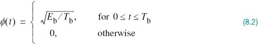
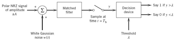
Figure 8.1 Receiver for baseband transmission of binary-encoded data stream using polar NRZ signaling.
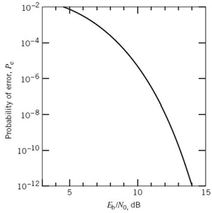
Figure 8.2 Probability of error in the signaling scheme of Figure 8.1.
In mathematical terms, the form of signaling embodied in Figure 8.1 is equivalent to that of binary PSK. Following (7.109), the average probability of symbol error incurred by the matched-filter receiver in Figure 8.1 is therefore defined by the Q-function
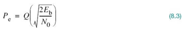
Although this result for NRZ-signaling over an AWGN channel may seem to be special, (8.3) holds for a binary data transmission system where symbol 1 is represented by a generic pulse g(t) and symbol 0 is represented by –g(t) under the assumption that the energy contained in g(t) is equal to Eb. This statement follows from matched-filter theory presented in Chapter 7.
Figure 8.2 plots Pe versus the dimensionless SNR, Eb/N0. The important message to take from this figure is summed up as follows:
The matched-filter receiver of Figure 8.1 exhibits an exponential improvement in the average probability of symbol error Pe with the increase in Eb/N0.
For example, expressing Eb/N0 in decibels we see from Figure 8.2 that Pe is on the order of 10–6 when Eb/N0 = 10 dB. Such a value of Pe is small enough to say that the effect of the channel noise is ignorable.
Henceforth, in the first part of the chapter dealing with signaling over band-limited channels, we assume that the SNR, Eb/N0, is large enough to leave intersymbol interference as the only source of interference.
8.3 Intersymbol Interference
To proceed with a mathematical study of intersymbol interference, consider a baseband binary PAM system, a generic form of which is depicted in Figure 8.3. The term “baseband” refers to an information-bearing signal whose spectrum extends from (or near) zero up to some finite value for positive frequencies. Thus, with the input data stream being a baseband signal, the data-transmission system of Figure 8.3 is said to be a baseband system. Consequently, unlike the subject matter studied in Chapter 7, there is no carrier modulation in the transmitter and, therefore, no carrier demodulation in the receiver to be considered.
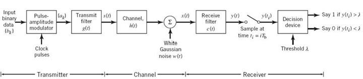
Figure 8.3 Baseband binary data transmission system.
Next, addressing the choice of discrete PAM, we say that this form of pulse modulation is one of the most efficient schemes for data transmission over a baseband channel when the utilization of both transmit power and channel bandwidth is of particular concern. In this section, we consider the simple case of binary PAM.
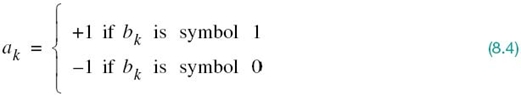
Referring back to Figure 8.3, the pulse-amplitude modulator changes the input binary data stream {bk} into a new sequence of short pulses, short enough to approximate impulses. More specifically, the pulse amplitude ak is represented in the polar form:
The sequence of short pulses so produced is applied to a transmit filter whose impulse response is denoted by g(t). The transmitted signal is thus defined by the sequence
Equation (8.5) is a form of linear modulation, which may be stated in words as follows:
A binary data stream represented by the sequence {ak}, where ak = +1 for symbol 1 and ak = –1 for symbol 0, modulates the basis pulse g(t) and superposes linearly to form the transmitted signal s(t).
The signal s(t) is naturally modified as a result of transmission through the channel whose impulse response is denoted by h(t). The noisy received signal x(t) is passed through a receive filter of impulse response c(t). The resulting filter output y(t) is sampled synchronously with the transmitter, with the sampling instants being determined by a clock or timing signal that is usually extracted from the receive-filter output. Finally, the sequence of samples thus obtained is used to reconstruct the original data sequence by means of a decision device. Specifically, the amplitude of each sample is compared with a zero threshold, assuming that the symbols 1 and 0 are equiprobable. If the zero threshold is exceeded, a decision is made in favor of symbol 1; otherwise a decision is made in favor of symbol 0. If the sample amplitude equals the zero threshold exactly, the receiver simply makes a random guess.
Except for a trivial scaling factor, we may now express the receive filter output as
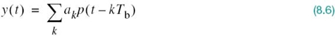
where the pulse p(t) is to be defined. To be precise, an arbitrary time delay t0 should be included in the argument of the pulse p(t – kTb) in (8.6) to represent the effect of transmission delay through the system. To simplify the exposition, we have put this delay equal to zero in (8.6) without loss of generality; moreover, the channel noise is ignored.
The scaled pulse p(t) is obtained by a double convolution involving the impulse response g(t) of the transmit filter, the impulse response h(t) of the channel, and the impulse response c(t) of the receive filter, as shown by
where, as usual, the star denotes convolution. We assume that the pulse p(t) is normalized by setting
which justifies the use of a scaling factor to account for amplitude changes incurred in the course of signal transmission through the system.
Since convolution in the time domain is transformed into multiplication in the frequency domain, we may use the Fourier transform to change (8.7) into the equivalent form
where P(ƒ), G(ƒ), H(ƒ), and C(ƒ) are the Fourier transforms of p(t), g(t), h(t), and c(t), respectively.
The receive filter output y(t) is sampled at time ti = iTb, where i takes on integer values; hence, we may use (8.6) to write
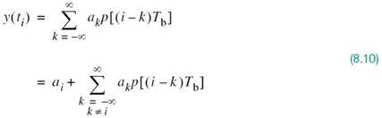
In (8.10), the first term ai represents the contribution of the ith transmitted bit. The second term represents the residual effect of all other transmitted bits on the decoding of the ith bit. This residual effect due to the occurrence of pulses before and after the sampling instant ti is called intersymbol interference (ISI).
In the absence of ISI—and, of course, channel noise—we observe from (8.10) that the summation term is zero, thereby reducing the equation to
![]()
which shows that, under these ideal conditions, the ith transmitted bit is decoded correctly.
8.4 Signal Design for Zero ISI
The primary objective of this chapter is to formulate an overall pulse shape p(t) so as to mitigate the ISI problem, given the impulse response of the channel h(t). With this objective in mind, we may now state the problem at hand:
Construct the overall pulse shape p(t) produced by the entire binary data-transmission system of Figure 8.3, such that the receiver is enabled to reconstruct the original data stream applied to the transmitter input exactly.
In effect, signaling over the band-limited channel becomes distortionless; hence, we may refer to the pulse-shaping requirement as a signal-design problem.
In the next section we describe a signal-design procedure, whereby overlapping pulses in the binary data-transmission system of Figure 8.3 are configured in such a way that at the receiver output they do not interfere with each other at the sampling times ti = iTb. So long as the reconstruction of the original binary data stream is accomplished, the behavior of the overlapping pulses outside these sampling times is clearly of no practical consequence. Such a design procedure is rooted in the criterion for distortionless transmission, which was formulated by Nyquist (1928b) on telegraph transmission theory, a theory that is as valid then as it is today.
Referring to (8.10), we see that the weighted pulse contribution, ak p(iTb – kTb), must be zero for all k except for k = 1 for binary data transmission across the band-limited channel to be ISI free. In other words, the overall pulse-shape p(t) must be designed to satisfy the requirement
where p(0) is set equal to unity in accordance with the normalization condition of (8.8). A pulse p(t) that satisfies the two-part condition of (8.11) is called a Nyquist pulse, and the condition itself is referred to as Nyquist’s criterion for distortionless binary baseband data transmission. However, there is no unique Nyquist pulse; rather, there are many pulse shapes that satisfy the Nyquist criterion of (8.11). In the next section we describe two kinds of Nyquist pulses, each with its own attributes.
8.5 Ideal Nyquist Pulse for Distortionless Baseband Data Transmission
From a design point of view, it is informative to transform the two-part condition of (8.11) into the frequency domain. Consider then the sequence of samples {p(nTb)}, where n = 0, ±1, ±2,… From the discussion presented in Chapter 6 on the sampling process, we recall that sampling in the time domain produces periodicity in the frequency domain. In particular, we may write
where Rb = 1/Tb is the bit rate in bits per second; Pδ(ƒ) on the left-hand side of (8.12) is the Fourier transform of an infinite periodic sequence of delta functions of period Tb whose individual areas are weighted by the respective sample values of p(t). That is, Pδ (ƒ) is given by

Let the integer m = i – k. Then, i = k corresponds to m = 0 and, likewise, i ≠ k corresponds to m ≠ 0. Accordingly, imposing the conditions of (8.11) on the sample values of p(t) in the integral in (8.13), we get
where we have made use of the sifting property of the delta function. Since from (8.8) we have p(0) = 1, it follows from (8.12) and (8.14) that the frequency-domain condition for zero ISI is satisfied, provided that
where Tb = 1Rb. We may now make the following statement on the Nyquist criterion1 for distortionless baseband transmission in the frequency domain:
The frequency function P(ƒ) eliminates inter symbol interference for samples taken at intervals Tb provided that it satisfies (8.15).
Note that P(ƒ) refers to the overall system, incorporating the transmit filter, the channel, and the receive filter in accordance with (8.9).
Ideal Nyquist Pulse
The simplest way of satisfying (8.15) is to specify the frequency function P(ƒ) to be in the form of a rectangular function, as shown by
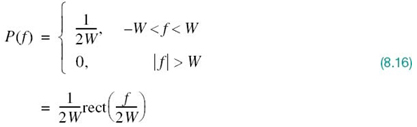
where rect(ƒ) stands for a rectangular function of unit amplitude and unit support centered on ƒ = 0 and the overall baseband system bandwidth W is defined by
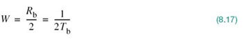
According to the solution in (8.16), no frequencies of absolute value exceeding half the bit rate are needed. Hence, from Fourier-transform pair 1 of Table 2.2 in Chapter 2, we find that a signal waveform that produces zero ISI is defined by the sinc function:
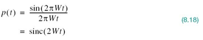
The special value of the bit rate Rb = 2W is called the Nyquist rate and W is itself called the Nyquist bandwidth. Correspondingly, the baseband pulse p(t) for distortionless transmission described in (8.18) is called the ideal Nyquist pulse, ideal in the sense that the bandwidth requirement is one half the bit rate.
Figure 8.4 shows plots of P(ƒ) and p(t). In part a of the figure, the normalized form of the frequency function P(ƒ) is plotted for positive and negative frequencies. In part b of the figure, we have also included the signaling intervals and the corresponding centered sampling instants. The function p(t) can be regarded as the impulse response of an ideal low-pass filter with passband magnitude response 1/2W and bandwidth W. The function p(t) has its peak value at the origin and goes through zero at integer multiples of the bit duration Tb. It is apparent, therefore, that if the received waveform y(t) is sampled at the instants of time t = 0, ±Tb, ± 2Tb,…, then the pulses defined by ai p(t – iTb) with amplitude ai and index i = 0, ±1, ±2,… will not interfere with each other. This condition is illustrated in Figure 8.5 for the binary sequence 1011010.
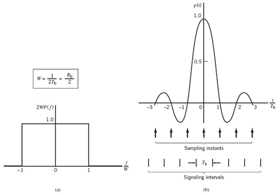
Figure 8.4 (a) Ideal magnitude response. (b) Ideal basic pulse shape.
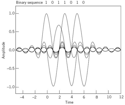
Figure 8.5 A series of sinc pulses corresponding to the sequence 1011010.
Although the use of the ideal Nyquist pulse does indeed achieve economy in bandwidth, in that it solves the problem of zero ISI with the minimum bandwidth possible, there are two practical difficulties that make it an undesirable objective for signal design:
1. It requires that the magnitude characteristic of P(ƒ) be flat from –W to +W, and zero elsewhere. This is physically unrealizable because of the abrupt transitions at the band edges ±W, in that the Paley–Wiener criterion discussed in Chapter 2 is violated.
2. The pulse function p(t) decreases as 1/|t| for large |t|, resulting in a slow rate of decay. This is also caused by the discontinuity of P(ƒ) at ±W. Accordingly, there is practically no margin of error in sampling times in the receiver.
To evaluate the effect of the timing error alluded to under point 2, consider the sample of y(t) at t = Δt, where Δt is the timing error. To simplify the exposition, we may put the correct sampling time ti equal to zero. In the absence of noise, we thus have from the first line of (8.10):
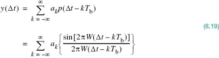
Since 2WTb = 1, by definition, we may reduce (8.19) to
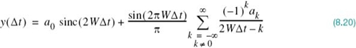
The first term on the right-hand side of (8.20) defines the desired symbol, whereas the remaining series represents the ISI caused by the timing error Δt in sampling the receiver output y(t). Unfortunately, it is possible for this series to diverge, thereby causing the receiver to make erroneous decisions that are undesirable.
8.6 Raised-Cosine Spectrum
We may overcom the practical difficulties encountered with the ideal Nyquist pulse by extending the bandwidth from the minimum value W = Rb/2 to an adjustable value between W and 2W. In effect, we are trading off increased channel bandwidth for a more robust signal design that is tolerant of timing errors. Specifically, the overall frequency response P(ƒ) is designed to satisfy a condition more stringent than that for the ideal Nyquist pulse, in that we retain three terms of the summation on the left-hand side of (8.15) and restrict the frequency band of interest to [–W, W], as shown by
where, on the right-hand side, we have set Rb = 1/2W in accordance with (8.17). We may now devise several band-limited functions that satisfy (8.21). A particular form of P(ƒ)that embodies many desirable features is provided by a raised-cosine (RC) spectrum. This frequency response consists of a flat portion and a roll-off portion that has a sinusoidal form, as shown by:
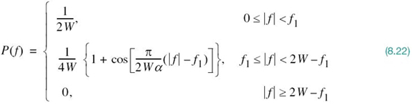
In (8.22), we have introduced a new frequency ƒ1 and a dimensionless parameter α, which are related by

The parameter α is commonly called the roll-off factor; it indicates the excess bandwidth over the ideal solution, W. Specifically, the new transmission bandwidth is defined by
The frequency response P(ƒ), normalized by multiplying it by the factor 2W, is plotted in Figure 8.6a for α = 0, 0.5, and 1. We see that for α = 0.5 or 1, the frequency response P(ƒ) rolls off gradually compared with the ideal Nyquist pulse (i.e., α = 0) and it is therefore easier to implement in practice. This roll-off is cosine-like in shape, hence the terminology “RC spectrum.” Just as importantly, the P(ƒ) exhibits odd symmetry with respect to the Nyquist bandwidth W, which makes it possible to satisfy the frequency-domain condition of (8.15).
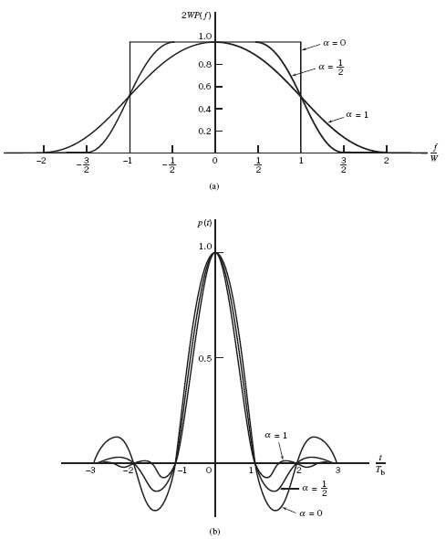
Figure 8.6 Responses for different roll-off factors: (a) frequency response; (b) time response.
The time response p(t) is naturally the inverse Fourier transform of the frequency response P(ƒ). Hence, transforming the P(ƒ) defined in (8.22) into the time domain, we obtain
which is plotted in Figure 8.6b for α = 0, 0.5, and 1.
The time response p(t) consists of the product of two factors: the factor sinc(2Wt) characterizing the ideal Nyquist pulse and a second factor that decreases as 1/|t|2 for large |t|. The first factor ensures zero crossings of p(t) at the desired sampling instants of time t = iTb, with i equal to an integer (positive and negative). The second factor reduces the tails of the pulse considerably below those obtained from the ideal Nyquist pulse, so that the transmission of binary data using such pulses is relatively insensitive to sampling time errors. In fact, for α = 1 we have the most gradual roll-off, in that the amplitudes of the oscillatory tails of p(t) are smallest. Thus, the amount of ISI resulting from timing error decreases as the roll-off factor α is increased from zero to unity.
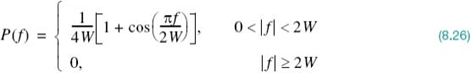
The special case with α = 1 (i.e., ƒ1 = 0) is known as the full-cosine roll-off characteristic, for which the frequency response of (8.22) simplifies to
Correspondingly, the time response p(t) simplifies to
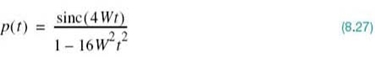
The time response of (8.27) exhibits two interesting properties:
1. At t = +Tb/2 = ±1/4W, we have p(t) = 0.5; that is, the pulse width measured at half amplitude is exactly equal to the bit duration Tb.
2. There are zero crossings at t = ±3Tb/2, ±5Tb/2,… in addition to the usual zero crossings at the sampling times t = ±Tb, ±2Tb,…
These two properties are extremely useful in extracting timing information from the received signal for the purpose of synchronization. However, the price paid for this desirable property is the use of a channel bandwidth double that required for the ideal Nyquist channel for which α = 0: simply put, there is “no free lunch.”
EXAMPLE 1 FIR Modeling of the Raised-Cosine Pulse
In this example, we use the finite-duration impulse response (FIR) filter, also referred to as the tapped-delay-line (TDL) filter, to model the raised-cosine (RC) filter; both terms are used interchangeably. With the FIR filter operating in the discrete-time domain, there are two time-scales to be considered:
1. Discretization of the input signal a(t) applied to the FIR model, for which we write
where T is the sampling period in the FIR model shown in Figure 8.7. The tap inputs in this model are denoted by![]() which, for some integer l, occupies the duration 2lT. Note that the FIR model in Figure 8.7 is symmetric about the midpoint, an −l, which satisfies the symmetric structure of the RC pulse.
which, for some integer l, occupies the duration 2lT. Note that the FIR model in Figure 8.7 is symmetric about the midpoint, an −l, which satisfies the symmetric structure of the RC pulse.
2. Discretization of the RC pulse p(t) for which we have
where Tb is the bit duration.
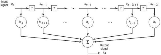
Figure 8.7 TDL model of linear time-invariant system.
To model the RC pulse properly, the sampling rate of the model, 1/T, must be higher than the bit rate, 1/Tb. It follows therefore that the integer m defined in (8.29) must be larger than one. In assigning a suitable value to m, we must keep in mind the tradeoff between modeling accuracy (requiring large m) and computational complexity (preferring small m).
In any event, using (8.17), (8.28), and (8.29), obtaining the product
and then substituting this result into (8.25), we get the discretized version of RC pulse as shown by
There are two computational difficulties encountered in the way in which the discretized RC pulse, pn, is defined in (8.31):
1. The pulse pn goes on indefinitely with increasing n.
2. The pulse is also noncausal in that the output signal yn in Figure 8.7 is produced before the input an is applied to the FIR model.
To overcome difficulty 1, we truncate the sequence pn such that it occupies a finite duration 2lT for some prescribed integer l, which is indeed what has been done in Figure 8.8. To mitigate the non-causality problem 2, with T >Tb, the ratio n/m must be replaced by (n/m) – l. In so doing, the truncated causal RC pulse assumes the following modified form:
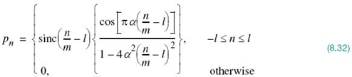
where the value assigned to the integer l is determined by how long the truncated sequence ![]() is desired to be.
is desired to be.
With the desired formula of (8.32) for the FIR model of the RC pulse p(t) at hand, Figure 8.8 plots this formula for the following specifications:2
Sampling of the RC pulse, T = 10
Bit duration of the RC pulse, Tb = 1
Number of the FIR samples per bit, m = 10
Roll-off factor of the RC pulse, α = 0.32
Two noteworthy points that follow from Figure 8.8:
1. The truncated causal RC pulse pn of length 2l – 10 is symmetric about the midpoint, n = 5.
2. The pn is exactly zero at integer multiples of the bit duration Tb.
Both points reaffirm exactly what we know and therefore expect about the RC pulse p(t) plotted in Figure 8.6b.
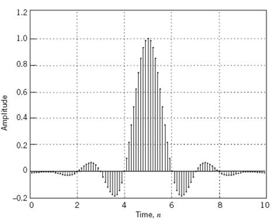
Figure 8.8 Discretized RC pulse, computed using the TDL.
8.7 Square-Root Raised-Cosine Spectrum
A more sophisticated form of pulse shaping uses the square-root raised-cosine (SRRC) spectrum3 rather than the conventional RC spectrum of (8.22). Specifically, the spectrum of the basic pulse is now defined by the square root of the right-hand side of this equation. Thus, using the trigonometric identity
![]()
where, for the problem at hand, the angle
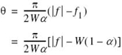
To avoid confusion, we use G(ƒ) as the symbol for the SRRC spectrum, and so we may write
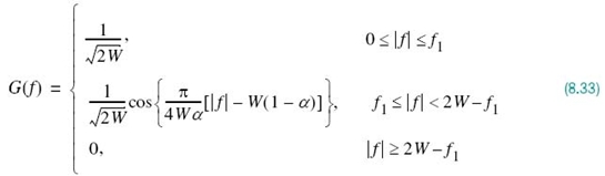
where, as before, the roll-off factor α is defined in terms of the frequency parameter ƒ1 and the bandwidth W as in (8.23).
If, now, the transmitter includes a pre-modulation filter with the transfer function defined in (8.33) and the receiver includes an identical post-modulation filter, then under ideal conditions the overall pulse waveform will experience the squared spectrum G2(ƒ), which is the regular RC spectrum. In effect, by adopting the SR RC spectrum G(ƒ) of (8.33) for pulse shaping, we would be working with G2(ƒ) = P(ƒ) in an overall transmitter–receiver sense. On this basis, we find that in wireless communications, for example, if the channel is affected by both fading and AWGN and the pulse-shape filtering is partitioned equally between the transmitter and the receiver in the manner described herein, then effectively the receiver would maximize the output SNR at the sampling instants.
The inverse Fourier transform of (8.33) defines the SRRC shaping pulse:
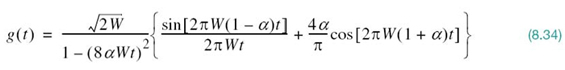
The important point to note here is the fact that the SRRC shaping pulse g(t) of (8.34) is radically different from the conventional RC shaping pulse of (8.25). In particular, the new shaping pulse has the distinct property of satisfying the orthogonality constraint under T-shifts, described by
where T is the symbol duration. Yet, the new pulse g(t) has exactly the same excess bandwidth as the conventional RC pulse.
It is also important to note, however, that despite the added property of orthogonality, the SRRC shaping pulse of (8.34) lacks the zero-crossing property of the conventional RC shaping pulse defined in (8.25).
Figure 8.9a plots the SRRC spectrum G(ƒ) for the roll-off factor α = 0, 0.5, 1; the corresponding time-domain plots are shown in Figure 8.9b. These plots are naturally different from those of Figure 8.6 for nonzero α. The following example contrasts the waveform of a specific binary sequence using the SRRC shaping pulse with the corresponding waveform using the regular RC shaping pulse.
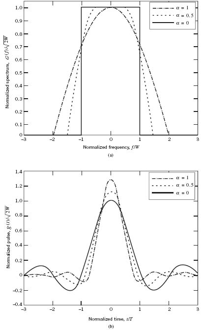
Figure 8.9 (a) G(ƒ) for SRRC spectrum. (b) g(t) for SRRC pulse.
EXAMPLE 2 Pulse Shaping Comparison Between SRRC and RC
Using the SRRC shaping pulse g(t) of (8.34) with roll-off factor α = 0.5, the requirement is to plot the waveform for the binary sequence 01100 and compare it with the corresponding waveform obtained by using the conventional RC shaping pulse p(t) of (8.25) with the same roll-off factor.
Using the SRRC pulse g(t) of (8.34) with a multiplying plus sign for binary symbol 1 and multiplying minus sign for binary symbol 0, we get the dashed pulse train shown in Figure 8.10 for the sequence 01100. The solid pulse train shown in the figure corresponds to the use of the conventional RC pulse p(t) of (8.25). The figure clearly shows that the SRRC waveform occupies a larger dynamic range than theconventional RC waveform: a feature that distinguishes one from the other.
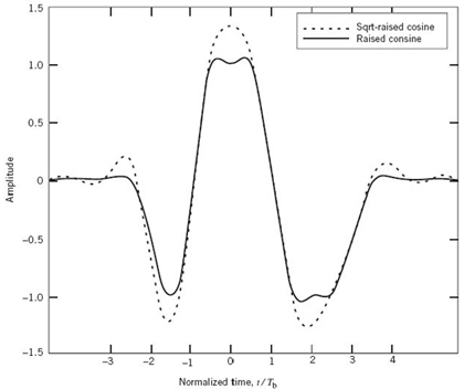
Figure 8.10 Two pulse trains for the sequence 01100, one using regular RC pulse (solid line), and the other using an SRRC pulse (dashed line).
EXAMPLE 3 FIR Modeling of the Square-Root-Raised-Cosine Pulse
In this example, we study FIR modeling of the SRRC pulse described in (8.34). To be specific, we follow a procedure similar to that used for the RC pulse g(t) in Example 1, taking care of the issues of truncation and noncausality. This is done by discretizing the SRRC pulse, g(t), and substituting the dimensionless parameter, (n/m) – l, for Wt in (8.34). In so doing we obtain the following sequence
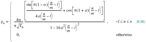
Since, by definition, the Fourier transform of the SRRC pulse, g(t), is equal to the square root of the Fourier transform of the RC pulse p(t), we may make the following statement:
The cascade connection of two identical FIR filters, each one defined by (8.36), is essentially equivalent to a TDL filter that exhibits zero intersymbol interference in accordance with (8.25).
We say “essentially” here on account of the truncation applied to both (8.32) and (8.36). In practice, when using the SRRC pulse for “ISI-free” baseband data transmission across a band-limited channel, one FIR filter would be placed in the transmitter and the other would be in the receiver.
To conclude this example, Figure 8.11a plots the SRRC sequence gn of (8.36) for the same set of values used for the RC sequence pn in Figure 8.8. Figure 8.11b displays the result of convolving the sequence in part a with gn, which is, itself.
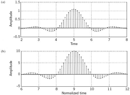
Figure 8.11 (a) Discretized SRRC pulse, computed using FIR modeling. (b) Discretized pulse resulting from the convolution of the pulse in part a with itself.
Two points are noteworthy from Figure 8.11:
1. The zero-crossings of the SRRC sequence gn do not occur at integer multiples of the bit duration Tb, which is to be expected.
2. The sequence plotted in Figure 8.11b is essentially equivalent to the RC sequence pn, the zero-crossings of which do occur at integer multiples of the bit duration, and so they should.
8.8 Post-Processing Techniques: The Eye Pattern
The study of signaling over band-limited channels would be incomplete without discussing the idea of post-processing, the essence of which is to manipulate a given set of data so as to provide a visual interpretation of the data rather than just numerical listing of the data. For an illustrative example, consider the formulas for the BER of digital modulation schemes operating over an AWGN channel, which were summarized in Table 7.7 of Chapter 7. The graphical plots of the schemes, shown in Figure7.47, provide an immediate comparison on how these different modulation schemes, compete with each other in terms of performance measured on the basis of their respective BERs for varying Eb/N0. In other words, there is much to be gained from graphical plots that are most conveniently made possible by computation.
What we have in mind in this section, however, is the description of a commonly used post-processor, namely eye patterns, which are particularly suited for the experimental study of digital communication systems.
The eye pattern, also referred to as the eye diagram, is produced by the synchronized superposition of (as many as possible) successive symbol intervals of the distorted waveform appearing at the output of the receive filter prior to thresholding. As an illustrative example, consider the distorted, but noise-free, waveform shown in part a of Figure 8.12. Part b of the figure displays the corresponding synchronized superposition of the waveform’s eight binary symbol intervals. The resulting display is called an “eye pattern” because of its resemblance to a human eye. By the same token, the interior of the eye pattern is called the eye opening.
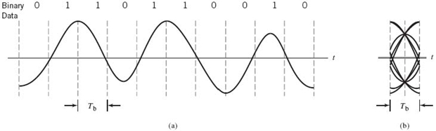
Figure 8.12 (a) Binary data sequence and its waveform. (b) Corresponding eye pattern.
As long as the additive channel noise is not large, then the eye pattern is well defined and may, therefore, be studied experimentally on an oscilloscope. The waveform under study is applied to the deflection plates of the oscilloscope with its time-base circuit operating in a synchronized condition. From an experimental perspective, the eye pattern offers two compelling virtues:
- The simplicity of eye-pattern generation.
- The provision of a great deal of insightful information about the characteristics of the data transmission system. Hence, the wide use of eye patterns as a visual indicator of how well or poorly a data transmission system performs the task of transporting a data sequence across a physical channel.
Timing Features
Figure 8.13 shows a generic eye pattern for distorted but noise-free binary data. The horizontal axis, representing time, spans the symbol interval from –T b/2 to Tb/2, where Tb is the bit duration. From this diagram, we may infer three timing features pertaining to a binary data transmission system, exemplified by a PAM system:
1. Optimum sampling time. The width of the eye opening defines the time interval over which the distorted binary waveform appearing at the output of the receive filter in the PAM system can be uniformly sampled without decision errors. Clearly, the optimum sampling time is the time at which the eye opening is at its widest.
2. Zero-crossing jitter. In practice, the timing signal (for synchronizing the receiver to the transmitter) is extracted from the zero-crossings of the waveform that appears at the receive-filter output. In such a form of synchronization, there will always be irregularities in the zero-crossings, which, in turn, give rise to jitter and, therefore, nonoptimum sampling times.
3. Timing sensitivity. Another timing-related feature is the sensitivity of the PAM system to timing errors. This sensitivity is determined by the rate at which the eye pattern is closed as the sampling time is varied.
Figure 8.13 indicates how these three timing features of the system (and other insightful attributes) can be measured from the eye pattern.
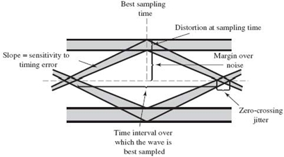
Figure 8.13 Interpretation of the eye pattern for a baseband binary data transmission system.
The Peak Distortion for Intersymbol Interference
Hereafter, we assume that the ideal signal amplitude is scaled to occupy the range from –1 to +1. We then find that, in the absence of channel noise, the eye opening assumes two extreme values:
1. An eye opening of unity,4 which corresponds to zero ISI.
2. An eye opening of zero, which corresponds to a completely closed eye pattern; this second extreme case occurs when the effect of intersymbol interference is severe enough for some upper traces in the eye pattern to cross with its lower traces.
It is indeed possible for the receiver to make decision errors even when the channel is noise free. Typically, an eye opening of 0.5 or better is considered to yield reliable data transmission.
In a noisy environment, the extent of eye opening at the optimum sampling time provides a measure of the operating margin over additive channel noise. This measure, as illustrated in Figure 8.13, is referred to as the noise margin.
From this discussion, it is apparent that the eye opening plays an important role in assessing system performance; hence the need for a formal definition of the eye opening. To this end, we offer the following definition:
where Dpeak denotes a new criterion called the peak distortion. The point to note here is that peak distortion is a worst-case criterion for assessing the effect of ISI on the performance (i.e., error rate) of a data transmission system. The relationship between the eye opening and peak distortion is illustrated in Figure 8.14. With the eye opening being dimensionless, the peak distortion is dimensionless too. To emphasize this statement, the two extreme values of the eye opening translate as follows:
1. Zero peak distortion, which occurs when the eye opening is unity.
2. Unity peak distortion, which occurs when the eye pattern is completely closed.
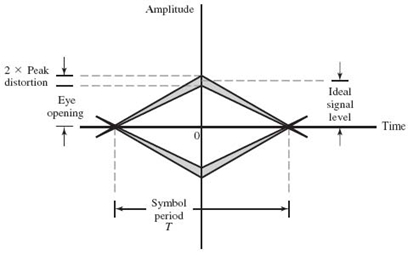
Figure 8.14 Illustrating the relationship between peak distortion and eye opening.
Note: the ideal signal level is scaled to lie inside the range –1 to +1.
With this background, we offer the following definition:
The peak distortion is the maximum value assumed by the intersymbol interference over all possible transmitted sequences, with this maximum value divided by a normalization factor equal to the absolute value of the corresponding signal level idealized for zero intersymbol interference.
Referring to (8.10), the two components embodied in this definition are themselves defined as follows:
1. The idealized signal component of the receive filter output is defined by the first term in (8.10), namely ai, where ai is the ith encoded symbol and unit transmitted signal energy per bit.
2. The intersymbol interference is defined by the second term, namely
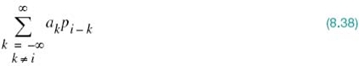
where pi – k stands for the term![]() The maximum value of this summation occurs when each encoded symbol ak has the same algebraic sign as pi – k. Therefore,
The maximum value of this summation occurs when each encoded symbol ak has the same algebraic sign as pi – k. Therefore,

Hence, invoking the definition of peak distortion, we get the desired formula:
where p0 = 1 for all i = k. Note that, by involving the assumption of a signal amplitude from –1 to +1, we have scaled the transmitted signal energy for a binary symbol to be unity.
By its very nature, the peak distortion is a worst-case criterion for data transmission over a noisy channel. The eye opening specifies the smallest possible noise margin.
Eye Patterns for M-ary Transmission
By definition, an M-ary data transmission system uses M encoded symbols in the transmitter and thresholds M – 1 in the receiver. Correspondingly, the eye pattern for an M-ary data transmission system contains M – 1 eye openings stacked vertically one on top of the other. The thresholds are defined by the amplitude-transition levels as we move up from one eye opening to the adjacent eye opening. When the encoded symbols are all equiprobable, the thresholds will be equidistant from each other.
In a strictly linear data transmission system with truly transmitted random data sequences, all the M – 1 eye openings would be identical. In practice, however, it is often possible to find asymmetries in the eye pattern of an M-ary data transmission system, which are caused by nonlinearities in the communication channel or other distortion-sensitive parts of the system.
EXAMPLE 4 Eye Patterns for Binary and Quaternary Systems
Figure 8.15a and b depict the eye patterns for a baseband PAM transmission system using M = 2 and M = 4, respectively. The channel has no bandwidth limitation and the source symbols used are obtained from a random number generator. An RC pulse is used in both cases. The system parameters used for the generation of these eye patterns are a bit rate of 1Hz and roll-off factor α = 0.5. For the binary case of M = 2 in Figure 8.15a, the symbol duration T and the bit duration Tb are the same, with Tb = 1s. For the case of M = 4 in Figure 8.15b we have T = Tblog2 M = 2Tb. In both cases we see that the eyes are open, indicating perfectly reliable operation of the system, perfect in the sense that the ISI is zero.
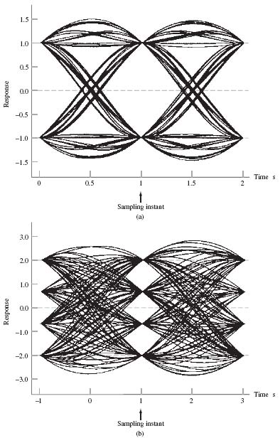
Figure 8.15 Eye diagrams of received signal with no bandwidth limitation: (a) M = 2; (b) M = 4.
Figure 8.16a and b show the eye patterns for these two baseband-pulse transmission systems using the same system parameters as before, but this time under a bandwidth-limited condition. Specifically, the channel is now modeled by a low-pass Butterworth filter, whose frequency response is defined by
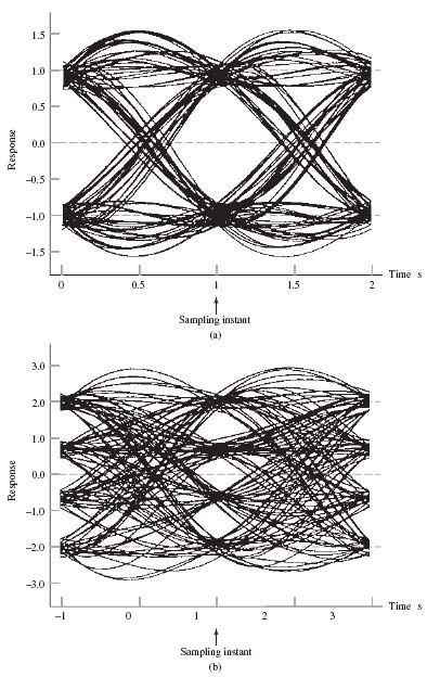
Figure 8.16 Eye diagrams of received signal, using a bandwidth-limited channel: (a) M = 2; (b) M = 4.

where N is the order of the filter, and ƒ0 is the 3-dB cutoff frequency of the filter. For the results displayed in Figure 8.16, the following filter parameter values were used:
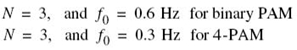
With the roll-off factor α = 0.5 and Nyquist bandwidth W = 0.5HZ, for binary PAM, the use of (8.24) defines the transmission bandwidth of the PAM transmission system to be
![]()
Although the channel bandwidth cutoff frequency is greater than absolutely necessary, its effect on the passband is observed in a decrease in the size of the eye opening. Instead of the distinct values at time t = 1s, shown in Figure 8.15a and b, now there is a blurred region. If the channel bandwidth were to be reduced further, the eye would close even more until finally no distinct eye opening would be recognizable.
8.9 Adaptive Equalization
In this section we develop a simple and yet effective algorithm for the adaptive equalization of a linear channel of unknown characteristics. Figure 8.17 shows the structure of an adaptive synchronous equalizer, which incorporates the matched filtering action. The algorithm used to adjust the equalizer coefficients assumes the availability of a desired response. One’s first reaction to the availability of a replica of the transmitted signal is: If such a signal is available at the receiver, why do we need adaptive equalization? To answer this question, we first note that a typical telephone channel changes little during an average data call. Accordingly, prior to data transmission, the equalizer is adjusted under the guidance of a training sequence transmitted through the channel. A synchronized version of this training sequence is generated at the receiver, where (after a time shift equal to the transmission delay through the channel) it is applied to the equalizer as the desired response. A training sequence commonly used in practice is the pseudonoise (PN) sequence, which consists of a deterministic periodic sequence with noise-like characteristics. Two identical PN sequence generators are used, one at the transmitter and the other at the receiver. When the training process is completed, the PN sequence generator is switched off and the adaptive equalizer is ready for normal data transmission. A detailed description of PN sequence generators is presented in Appendix J.

Figure 8.17 Block diagram of adaptive equalizer using an adjustable TDL filter.
Least-Mean-Square Algorithm (Revisited)
To simplify notational matters, we let

Then, the output yn of the tapped-delay-line (TDL) equalizer in response to the input sequence {xn} is defined by the discrete convolution sum (see Figure 8.17)
where wk is the weight at the kth tap and N + 1 is the total number of taps. The tap weights constitute the adaptive equalizer coefficients. We assume that the input sequence xn has finite energy. We have used a notation for the equalizer weights in Figure 8.17 that is different from the corresponding notation in Figure 6.17 to emphasize the fact that the equalizer in Figure 8.17 also incorporates matched filtering.
The adaptation may be achieved by observing the error between the desired pulse shapeand the actual pulse shape at the equalizer output, measured at the sampling instants, andthen using this error to estimate the direction in which the tap weights of the equalizer should be changed so as to approach an optimum set of values. For the adaptation, we may use a criterion based on minimizing the peak distortion, defined as the worst-case intersymbol interference at the output of the equalizer. However, the equalizer so designed is optimum only when the peak distortion at its input is less than 100% (i.e., the intersymbol interference is not too severe). A better approach is to use a mean-square error criterion, which is more general in application; also, an adaptive equalizer based on the mean-square error (MSE) criterion appears to be less sensitive to timing perturbations than one based on the peak-distortion criterion. Accordingly, in what follows we use the MSE criterion to derive the adaptive equalization algorithm.
Let an denote the desired response defined as the polar representation of the nth transmitted binary symbol. Let en denote the error signal defined as the difference between the desired response an and the actual response yn of the equalizer, as shown by
In the least-mean-square (LMS) algorithm for adaptive equalization, the error signal en actuates the adjustments applied to the individual tap weights of the equalizer as the algorithm proceeds from one iteration to the next. A derivation of the LMS algorithm for adaptive prediction was presented in Section 6.7 of Chapter 6. Recasting (6.85) into its most general form, we may restate the formula for the LMS algorithm in words as follows:
Let μ denote the step-size parameter. From Figure 8.17 we see that the input signal applied to the kth tap weight at time step n is xn – k. Hence, using ŵk(n) as the old value of the kth tap weight at time step n, the updated value of this tap weight at time step n + 1 is, in light of (8.43), defined by
where
These two equations constitute the LMS algorithm for adaptive equalization.
We may simplify the formulation of the LMS algorithm using matrix notation. Let the (N + 1)-by-1 vector xn denote the tap inputs of the equalizer:
where the superscript T denotes matrix transposition. Correspondingly, let the (N + 1)-by-1 vector ŵn denote the tap weights of the equalizer:
We may then use matrix notation to recast the discrete convolution sum of (8.41) in the compact form
where xTnŵn is referred to as the inner product of the vectors xn and ŵn. We may now summarize the LMS algorithm for adaptive equalization as follows:
1. Initialize the algorithm by setting ŵ1 = 0 (i.e., set all the tap weights of the equalizer to zero at n = 1, which corresponds to time t = T.
2. For n = 1,2,…,compute
where μ is the step-size parameter.
3. Continue the iterative computation until the equalizer reaches a “steady state, ” by which we mean that the actual mean-square error of the equalizer essentially reaches a constant value.
The LMS algorithm is an example of a feedback system, as illustrated in the block diagram of Figure 8.18, which pertains to the kth filter coefficient. It is therefore possible for the algorithm to diverge (i.e., for the adaptive equalizer to become unstable). Unfortunately, the convergence behavior of the LMS algorithm is difficult to analyze. Nevertheless, provided that the step-size parameter µ is assigned a small value, we find that after a large number of iterations the behavior of the LMS algorithm is roughly similar to that of the steepest-descent algorithm (discussed in Chapter 6), which uses the actual gradient rather than a noisy estimate for the computation of the tap weights.
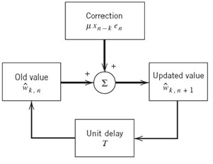
Figure 8.18 Signal-flow graph representation of the LMS algorithm involving the kth tap weight.
Operation of the Equalizer
There are two modes of operation for an adaptive equalizer, namely the training mode and decision-directed mode, as shown in Figure 8.19. During the training mode, a known PN sequence is transmitted and a synchronized version of it is generated in the receiver, where (after a time shift equal to the transmission delay) it is applied to the adaptive equalizer as the desired response; the tap weights of the equalizer are thereby adjusted in accordance with the LMS algorithm.
When the training process is completed, the adaptive equalizer is switched to its second mode of operation: the decision-directed mode. In this mode of operation, the error signal is defined by
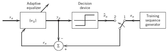
Figure 8.19 Illustrating the two operating modes of an adaptive equalizer: for the training mode, the switch is in position 1; for the tracking mode, it is moved to position 2.
where yn is the equalizer output at time t = nT and ân is the final (not necessarily) correct estimate of the transmitted symbol an. Now, in normal operation the decisions made by the receiver are correct with high probability. This means that the error estimates are correct most of the time, thereby permitting the adaptive equalizer to operate satisfactorily. Furthermore, an adaptive equalizer operating in a decision-directed mode is able to track relatively slow variations in channel characteristics.
It turns out that the larger the step-size parameter µ is, the faster the tracking capability of the adaptive equalizer. However, a large step-size parameter µ may result in an unacceptably high excess mean-square error, defined as that part of the mean-square value of the error signal in excess of the minimum attainable value, which results when the tap weights are at their optimum settings. We therefore find that, in practice, the choice of a suitable value for the step-size parameter µ involves making a compromise between fast tracking and reducing the excess mean-square error.
Decision-Feedback Equalization5
To develop further insight into adaptive equalization, consider a baseband channel with impulse response denoted in its sampled form by the sequence {hn}, where hn = h(nT). The response of this channel to an input sequence {xn}, in the absence of noise, is given by the discrete convolution sum
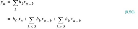
The first term of (8.50) represents the desired data symbol. The second term is due to the precursors of the channel impulse response that occur before the main sample h0 associated with the desired data symbol. The third term is due to the postcursors of the channel impulse response that occur after the main sample h0. The precursors and postcursors of a channel impulse response are illustrated in Figure 8.20. The idea of decision-feedback equalization is to use data decisions made on the basis of precursors of the channel impulse response to take care of the postcursors; for the idea to work, however, the decisions would obviously have to be correct for the DFE to function properly most of the time.
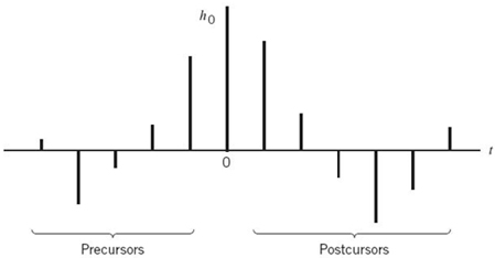
Figure 8.20 Impulse response of a discrete-time channel, depicting the precursors and postcursors.

Figure 8.21 Block diagram of decision-feedback equalizer.
A DFE consists of a feedforward section, a feedback section, and a decision device connected together as shown in Figure 8.21. The feedforward section consists of a TDL filter whose taps are spaced at the reciprocal of the signaling rate. The data sequence to be equalized is applied to this section. The feedback section consists of another TDL filter whose taps are also spaced at the reciprocal of the signaling rate. The input applied to the feedback section consists of the decisions made on previously detected symbols of the input sequence. The function of the feedback section is to subtract out that portion of the intersymbol interference produced by previously detected symbols from the estimates of future samples.
Note that the inclusion of the decision device in the feedback loop makes the equalizer intrinsically nonlinear and, therefore, more difficult to analyze than an ordinary LMS equalizer. Nevertheless, the mean-square error criterion can be used to obtain a mathematically tractable optimization of a DFE. Indeed, the LMS algorithm can be used to jointly adapt both the feedforward tap weights and the feedback tap weights based on a common error signal.
8.10 Broadband Backbone Data Network: Signaling over Multiple Baseband Channels
Up to this point in the chapter, the discussion has focused on signaling over a single band-limited channel and related issues such as adaptive equalization. In order to set the stage for the rest of the chapter devoted to signaling over a linear broadband channel purposely partitioned into a set of subchannels, this section on the broadband backbone data network (PSTN) is intended to provide a transition from the first part of the chapter to the second part.
The PSTN was originally built to provide a ubiquitous structure for the digital transmission of voice signals using PCM, which was discussed previously in Chapter 6. As such, traditionally, the PSTN has been viewed as an analog network. In reality, however, the PSTN has evolved into an almost entirely digital network. We say “almost entirely” because the analog refers to the local network, which stands for short-connections from a home to the central office.
For many decades past, data transmission over the PSTN relied on the use of modems; the term “modem” is a contraction of modulator–demodulator. Despite the enormous effort that was put into the design of modems, they could not cope with the ever-increasing rate of data transmission. This situation prevailed until the advent of digital subscriber line (DSL) technology in the 1990s. The inquisitive reader may well ask the question: How was it that the modem theorists and designers got it wrong while the DSL theorists and designers got it right? Unfortunately, in the development of modems, the telephone channel was treated as one whole entity. On the other hand, the development of DSL abandoned the traditional approach by viewing the telephone channel as a conglomeration of subchannels extending over a wide frequency band and operating in parallel, and with each subchannel treated as a narrowband channel, thereby exploiting Shannon’s information capacity law in a much more effective manner.
It is therefore not surprising that the DSL technology has converted an ordinary telephone line into a broadband communication link, so much so that we may now view the PSTN effectively as a broadband backbone data network, which is being widely used all over the world. The data consist of digital signals generated by computers or Internet service providers (ISPs). Most importantly, the deployment of DSL technology has literally made it possible to increase the rate of data transmission across a telephone channel by orders of magnitude compared with the old modems. This transition from modem to DSL technology is indeed an impressive engineering accomplishment, which resulted from “thinking outside the box.”
With this brief historical account, it is apropos that we devote the rest of the chapter to the underlying theory of the widely used DSL technology.
8.11 Digital Subscriber Lines
The term DSL is commonly used to refer to a family of different technologies that operate over a local loop less than 1.5 km to provide for digital signal transmission between a user terminal (e.g., computer) and the central office (CO) of a telephone company. Through the CO, the user is connected directly to the so-called broadband backbone data network, whereby transmission is maintained in the digital domain. In the course of transmission, the digital signal is switched and routed at regular intervals. Figure 8.22 is a schematic diagram illustrating that typically the data rate upstream (i.e., in the direction of the ISP) is lower than the data rate downstream (i.e., in the direction of the user). It is for this reason that the DSL is said to be asymmetric;6 hence the acronym ADSL.
The twisted wire-pair used in the local loop, the only analog part of the data transmission system as remarked earlier, is inductively loaded. Specifically, extra inductance is purposely supplied by local coils, which are inserted at regular intervals across the wire-pair. This addition is made in order to produce a fairly flat frequency response across the effective voice band. However, the improvement so gained for the transmission of voice signals is attained at the expense of continually increasing attenuation at frequencies higher than 3.4 kHz. Figure 8.23a illustrates the two different frequency bands allocated to a frequency-division multiplexive (FDM)-based ADSL; the way in which two filters, one high-pass and the other low-pass, are used to connect the DSL to the local loop is shown in Figure 8.23b.
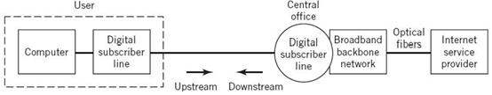
Figure 8.22 Block diagram depicting the operational environment of DSL.
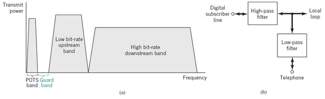
Figure 8.23 (a) Illustrating the different band allocations for an FDM-based ADSL system. (b) Block diagram of splitter performing the function of a multiplexer or demultiplexer.
Note: both filters in the splitter are bidirectional filters.
With access to the wide band represented by frequencies higher than 3.6 kHz, the DSL uses discrete multicarrier transmission (DMT) techniques to convert the twisted wire-pair in the local loop into a broadband communication link; the two terms “multichannel” and “multicarrier” are used interchangeably. The net result is that data rates of 1.5 to 9.0 Mbps downstream in a bandwidth of up to 1 MHz and over a distance of 2.7 to 5.5 km. Very high-bit-rate digital subscriber lines7 (VDSLs) do even better, supporting data rates of 13 to 52 Mbps downstream in a bandwidth of up to 30 MHz and over a distance of 0.3 to 1.5 km. These numbers indicate that the data rates attainable by DSL technology depend on both bandwidth and distance, and the technology continues to improve.
The basic idea behind DMT is rooted in a commonly used engineering paradigm:
Divide and conquer.
According to this paradigm, a difficult problem is solved by dividing it into a number of simpler problems and then combining the solutions to those simple problems. In the context of our present discussion, the difficult problem is that of data transmission over a wideband channel with severe intersymbol interference, and the simpler problems are exemplified by data transmission over relatively straightforward AWGN channels. We may thus describe the essence of DMT theory, as follows:
Data transmission over a difficult channel is transformed through the use of advanced signal processing techniques into the parallel transmission of the given data stream over a large number of subchannels, such that each subchannel may be viewed effectively as an AWGN channel.
Naturally, the overall data rate is the sum of the individual data rates over the subchannels designed to operate in parallel: this new way of thinking on signaling over wideband channels is entirely different from the approach described in the first part of the chapter, in that it builds on ideas described in Chapter 5 on Shannon’s information theory and in Chapter 7 on signaling over AWGN channels.
8.12 Capacity of AWGN Channel Revisited
At the heart of discrete multichannel data transmission theory is Shannon’s information capacity law, discussed in Chapter 5 on information theory. According to this law, the capacity of an AWGN channel (free from ISI) is defined by
where B is the channel bandwidth in hertz and SNR is measured at the channel output. Equation (8.51) teaches us that, for a given SNR, we can transmit data over an AWGN channel of bandwidth B at the maximum rate of B bit/s with arbitrarily small probability of error, provided that we employ an encoding system of sufficiently high complexity. Equivalently, we may express the capacity C in bits per transmission of channel use as
In practice, we usually find that a physically realizable encoding system must transmit data at a rate R less than the maximum possible rate C for it to be reliable. For an implementable system operating at low enough probability of symbol error, we thus need to introduce an SNR gap or just gap, denoted by Γ. The gap is a function of the permissible probability of symbol error Pe and the encoding system of interest. It provides a measure of the “efficiency” of an encoding system with respect to the ideal transmission system of (8.52). With C denoting the capacity of the ideal encoding system and R denoting the capacity of the corresponding implementable encoding system, the gap is defined by
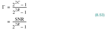
Rearranging (8.53) with R as the focus of interest, we may write
For an encoded PAM or QAM operating at Pe = 10–6, for example, the gap Γ is constant at 8.8 dB. Through the use of codes (e.g., trellis codes to be discussed in Chapter 10), the gap Γ may be reduced to as low as 1 dB.
Let P denote the transmitted signal power and σ2 denote the channel noise variance measured over the bandwidth B. The SNR is therefore

![]()
We may thus finally define the attainable data rate as
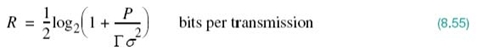
With this modified version of Shannon’s information capacity law at hand, we are ready to describe discrete multichannel modulation in quantitative terms.
8.13 Partitioning Continuous-Time Channel into a Set of Subchannels
To be specific in practical terms, consider a linear wideband channel (e.g., twisted wire-pair) with an arbitrary frequency response H(ƒ). Let the magnitude response of the channel, denoted by |H(ƒ)|, be approximated by a staircase function as illustrated in Figure 8.24, with Δƒ denoting the width of each frequency step (i.e., subchannel). In the limit, as the frequency increment Δƒ approaches zero, the staircase approximation of the channel approaches the actual H(ƒ). Along each step of the approximation, the channel may be assumed to operate as an AWGN channel free from intersymbol interference. The problem of transmitting a single wideband signal is thereby transformed into the transmission of a set of narrowband orthogonal signals. Each orthogonal narrowband signal, with its own carrier, is generated using a spectrally efficient modulation technique such as M-ary QAM, with AWGN being essentially the only primary source of transmission impairment. This scenario, in turn, means that data transmission over each subchannel of bandwidth Δƒ can be optimized by invoking a modified form of Shannon’s information capacity law, with the optimization of each subchannel being performed independently of all the others. Thus, in practical signal-processing terms, we may make the following statement:
The need for complicated equalization of a wideband channel is replaced by the need for multiplexing and demultiplexing the transmission of an incoming data stream over a large number of narrowband subchannels that are continuous and disjoint.
Although the resulting complexity of a DMT system so described is indeed high for a large number of subchannels, implementation of the entire system can be accomplished in a cost-effective manner through the combined use of efficient digital signal-processing algorithms and very-large-scale integration technology.
Figure 8.25 shows a block diagram of the DMT system in its most basic form. The system configured here uses QAM, whose choice is justified by virtue of its spectral efficiency. The incoming binary data stream is first applied to a demultiplexer (not shown in the figure), thereby producing a set of N substreams. Each substream represents a sequence of two-element subsymbols, which, for the symbol interval 0 ≤ t ≤ T, is denoted by
![]()
where an and bn are element values along the two coordinates of subchannel n.
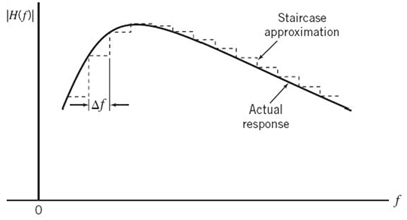
Figure 8.24 Staircase approximation of an arbitrary magnitude response of a channel, |H(ƒ)|; only positive-frequency portion of the response is shown.
Correspondingly, the passband basis functions of the quadrature-amplitude modulators are defined by the following function pairs:
The carrier frequency ƒn of the nth modulator described in (8.56) is an integer multiple of the symbol rate 1/T, as shown by
![]()
and the low-pass function ϕ(t), common to all the subchannels, is the sinc function
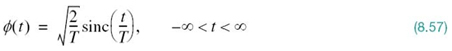
The passband basis functions defined here have the following desirable properties, whose proofs are presented as an end-of-chapter problem.
PROPERTY 1 For each n, the two quadrature-modulated sinc functions form an orthogonal pair, as shown by

This orthogonal relationship provides the basis for formulating the signal constellation for each of the N modulators in the form of a squared lattice.
PROPERTY 2 Recognizing that
![]()
we may completely redefine the passband basis functions in the complex form

where the factor ![]() has been introduced to ensure that the scaled function
has been introduced to ensure that the scaled function![]() has unit energy. Hence, these passband basis functions form an orthonormal set, as shown by
has unit energy. Hence, these passband basis functions form an orthonormal set, as shown by

The asterisk assigned to the second factor on the left-hand side denotes complex conjugation.
Equation (8.60) provides the mathematical basis for ensuring that the N modulator-demodulator pairs operate independently of each other.
PROPERTY 3 The set of channel-output functions remains orthogonal for a linear channel with arbitrary impulse response h(t), where
  denotes convolution.
Thus, in light of these three properties, the original wideband channel is partitioned into an ideal setting of independent subchannels operating in continuous time.
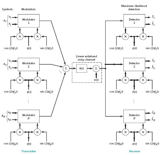
Figure 8.25 Block diagram of DMT system.
Figure 8.25 also includes the corresponding structure of the receiver. It consists of a bank of N coherent detectors, with the channel output being simultaneously applied to the detector inputs, operating in parallel. Each detector is supplied with a locally generated pair of quadrature-modulated sinc functions operating in synchrony with the pair of passband basis function applied to the corresponding modulator in the transmitter.
It is possible for each subchannel to have some residual ISI. However, as the number of subchannels N approaches infinity, the ISI disappears for all practical purposes. From a theoretical perspective, we find that, for a sufficiently large N, the bank of coherent detectors in Figure 8.25 operates as maximum likelihood detectors, operating independently of each other and on a subsymbol-by-subsymbol basis. (Maximum likelihood detection was discussed in Chapter 7.)
To define the detector outputs in response to the input subsymbols, we find it convenient to use complex notation. Let An denote the subsymbol applied to the nth modulator during the symbol interval 0 ≤ t ≤ T, as shown by
The corresponding detector output is expressed as follows:
where Hn is the complex-valued frequency response of the channel evaluated at the subchannel carrier frequency f = fn, that is,
The Wn in (8.62) is a complex-valued random variable produced by the channel noise w(t); the real and imaginary parts of Wn have zero mean and variance N0/2. With knowledge of the measured frequency response H(ƒ) available, we may therefore use (8.62) to compute a maximum likelihood estimate of the transmitted subsymbol An. The estimates ![]() so obtained are finally multiplexed to produce the overall estimate of the original binary data transmitted during the interval 0 ≤ t ≤ T.
so obtained are finally multiplexed to produce the overall estimate of the original binary data transmitted during the interval 0 ≤ t ≤ T.
To summarize, for a sufficiently large N, we may implement the receiver as an optimum maximum likelihood detector that operates as N subsymbol-by-subsymbol detectors. The rationale for building a maximum likelihood receiver in such a simple way is motivated by the following property:
PROPERTY 4 The passband basis functions constitute an orthonormal set and their orthogonality is maintained for any channel impulse response h(t).
Geometric SNR
In the DMT system of Figure 8.25, each subchannel is characterized by an SNR of its own. It would be highly desirable, therefore, to derive a single measure for the performance of the entire system in Figure 8.25.
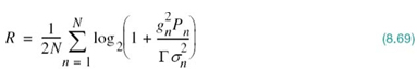
To simplify the derivation of such a measure, we assume that all of the subchannels in Figure 8.25 are represented by one-dimensional constellations. Then, using the modified Shannon information capacity law of (8.55), the channel capacity of the entire system is successively expressed as follows:
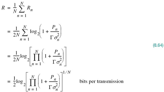
Let (SNR)overall denote the overall SNR of the entire DMT system. Then, in light of (8.54), we may express the rate R as
Accordingly, comparing (8.65) with (8.64) and rearranging terms, we may write
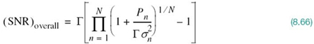
Assuming that the SNR, namely ![]() , is large enough to ignore the two unity terms on the right-hand side of (8.66), we may approximate the overall SNR simply as follows:
, is large enough to ignore the two unity terms on the right-hand side of (8.66), we may approximate the overall SNR simply as follows:

which is independent of the gap Γ. We may thus characterize the overall system by an SNR that is the geometric mean of the SNRs of the individual subchannels.
The geometric form of the SNR of (8.67) can be improved considerably by distributing the available transmit power among the N subchannels on a nonuniform basis. This objective is attained through the use of loading, which is discussed next.
Loading of the DMT System
Equation (8.64) for the bit rate of the entire DMT system ignores the effect of the channel on system performance. To account for this effect, define
Then, assuming that the number of subchannels N is large enough, we may treat gn as a constant over the entire bandwidth Δƒ assigned to subchannel n for all n. In such a case, we may modify the second line of (8.64) for the overall SNR of the system into
where the gn2 and Γ are usually fixed. The noise variance σn2 is Δf N0 for all n, whereΔf is the bandwidth of each subchannel and N0/2 is the noise power spectral density of the subchannel. We may therefore optimize the overall bit rate R through a proper allocation of the total transmit power among the various subchannels. However, for this optimization to be of practical value, we must maintain the total transmit power at some constant value denoted by P, as shown by
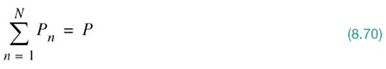
The optimization we therefore have to deal with is a constrained optimization problem, stated as follows:
Maximize the bit rate R for the DMT system through an optimal sharing of the total transmit power P between the N subchannels, subject to the constraint that the total transmit power P is maintained constant.
To solve this optimization problem, we first use the method of Lagrange multipliers8 to set up an objective function (i.e., the Lagrangian) that incorporates (8.69) and the constraint of (8.70) as shown by
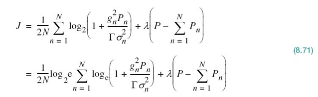
where λ is the Lagrange multiplier; in the second line of (8.71) the logarithm to base 2 has been changed to the natural logarithm written as log2e. Hence, differentiating the Lagrangian J with respect to Pn, then setting the result equal to zero and finally rearranging terms, we get
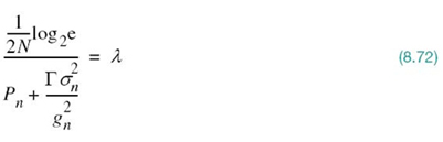
The result of (8.72) indicates that the solution to our constrained optimization problem is to have
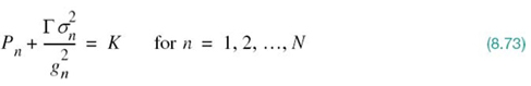
where K is a prescribed constant under the designer’s control. That is, the sum of the transmit power and the noise variance (power) scaled by the ratio Γ/gn2 must be maintained constant for each subchannel. The process of allocating the transmit power P to the individual subchannels so as to maximize the bit rate of the entire multichannel transmission system is called loading; this term is not to be confused with loading coils used in twisted wire-pairs.
8.14 Water-Filling Interpretation of the Constrained Optimization Problem
In solving the constrained optimization problem just described, the two conditions of (8.70) and (8.73) must both be satisfied. The optimum solution so defined has an interesting interpretation, as illustrated in Figure 8.26 for N = 6, assuming that the gap is maintained constant over all the subchannels. To simplify the illustration in Figure 8.26, we have set σn2 = N0Δƒ = 1; that is, the average noise power is unity for all Nsubchannels. Referring to this figure, we may now make three observations:
1. With σn2 = 1, the sum of power Pn allocated to subchannel n and the scaled noise power Г/gn2 satisfies the constraint of (8.73) for four of the subchannels for a prescribed value of the constant K.
2. The sum of power allocations to these four subchannels consumes all the available transmit power, maintained at the constant value P.
3. The remaining two subchannels have been eliminated from consideration because they would each require negative power to satisfy (8.73) for the prescribed value of the constant K; from a physical perspective, this condition is clearly unacceptable.
The interpretation illustrated in Figure 8.26 prompts us to refer to the optimum solution of (8.73), subject to the constraint of (8.70), as the water-filling solution; the principle of water-filling was discussed under Shannon’s information theory in Chapter 5. This terminology follows from analogy of our optimization problem with a fixed amount of water—standing for transmit power—being poured into a container with a number of connected regions, each having a different depth—standing for noise power. In such a scenario, the water distributes itself in such a way that a constant water level is attained across the whole container, hence the term “water filling.”
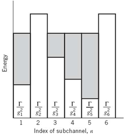
Figure 8.26 Water-filling interpretation of the loading problem.
Returning to the task of how to allocate the fixed transmit power P among the various subchannels of a multichannel data transmission system so as to optimize the bit rate of the entire system, we may proceed along the following pair of steps:
1. Let the total transmit power be fixed at the constant value P as in (8.70).
2. Let K denote the constant value prescribed for the sum, ![]() for all n as in (8.73).
for all n as in (8.73).
On the basis of these two steps, we may then set up the following system of simultaneous equations;
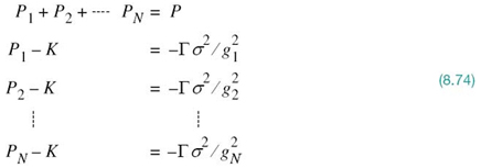
where we have a total of (N + 1) unknowns and (N + 1) equations to solve for them. Using matrix notation, we may rewrite this system of N + K simultaneous equations in the compact form
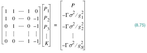
Premultiplying both sides of (8.75) by the inverse of the (N + 1)-by-(N + 1) matrix on the left-hand side of the equation, we obtain solutions for the unknowns P1, P2,…,PN, and K. We should always find that K is positive, but it is possible for some of the P values to be negative. In such a situation, the negative P values are discarded as power cannot be negative for physical reasons.
EXAMPLE 5 Linear Channel with Squared Magnitude Response
Consider a linear channel whose squared magnitude response |H(ƒ)|2 has the piecewise-linear form shown in Figure 8.27. To simplify the example, we have set the gap Г = 1 and the noise variance σ2 = 1.
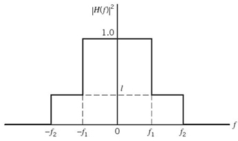
Figure 8.27 Squared magnitude response for Example 5.
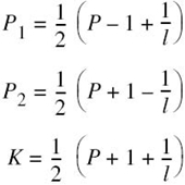
Under this set of values, the application of (8.74) yields
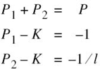
where the new parameter 0 < l < 1 has been introduced to distinguish the third equation from the second one. Solving these three simultaneous equations for P1, P2, and K, we get
Since 0 < l < 1, it follows that P1 > 0, but it is possible for P2 to be negative. This latter condition can arise if
![]()
But then P1 exceeds the prescribed value of transmit power P. Therefore, it follows that, in this example, the only acceptable solution is to have l/(P + 1) < l < 1. Suppose then we have P = 10 and l = 0.1; under these two conditions the desired solution is

The corresponding water-filling picture for the problem at hand is portrayed in Figure 8.28.
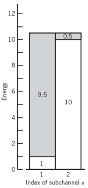
Figure 8.28 Water-filling profile for Example 5.
8.15 DMT System using Discrete Fourier Transform
The material presented in Sections 8.13 and 8.14 provides an insightful introduction to the notion of multicarrier modulation in a DMT system. In particular, the continuous-time channel partitioning induced by the passband (modulated) basis functions of (8.56), or equivalently (8.59) in complex terms, exhibits a highly desirable property described as follows:
Orthogonality of the basis functions, and therefore the channel partitioning, is preserved despite their individual convolutions with the impulse response of the channel.
However, the DSL system so described has two practical shortcomings:
1. The passband basis functions use a sinc function that is nonzero for an infinite time interval, whereas practical considerations favor a finite observation interval.
2. For a finite number of subchannels N the system is suboptimal; optimality of the system is assured only when N approaches infinity.
We may overcome both shortcomings by using DMT, the basic idea of which is to transform a noisy wideband channel into a set of N subchannels operating in parallel. What makes DMT distinctive is the fact that the transformation is performed in discrete time as well as discrete frequency, paving the way for exploiting digital signal processing. Specifically, the transmitter’s input–output behavior of the entire communication system admits a linear matrix representation, which lends itself to implementation using the DFT. In the following we know from Chapter 2 on Fourier analysis of signals and systems that the DFT is the result of discretizing the Fourier transform both in time and frequency.
To exploit this new approach, we first recognize that in a realistic situation the channel has its nonzero impulse response h(t) essentially confined to a finite interval [0, Tb]. So, let the sequence h0, h1,…,hv denote the baseband equivalent impulse response of the channel sampled at the rate 1/Ts, with
where the role of ν is to be clarified. The sampling rate 1/Ts is chosen to be greater than twice the highest frequency component of interest in accordance with the sampling theorem. To continue with the discrete-time description of the system, let sn = s(nTs)denote a sample of the transmitted symbol s(t), wn = w(nTs) denote a sample of the channel noise w(t), and xn = x(nTs) denote the corresponding sample of the channel output (i.e., received signal). The channel performs linear convolution on the incoming symbol sequence {sn} of length N to produce a channel output sequence{xn} of length N +ν. Extension of the channel output sequence by ν samples compared with the channel input sequence is due to the intersymbol interference produced by the channel.
To overcome the effect of ISI, we create a cyclically extended guard interval, whereby each symbol sequence is preceded by a periodic extension of the sequence itself. Specifically, the last νsamples of the symbol sequence are repeated at the beginning of the sequence being transmitted, as shown by
The condition described in (8.77) is called a cyclic prefix. The excess bandwidth factor due to the inclusion of the cyclic prefix is therefore ν/N, where N is the number of transmitted samples after the guard interval.
With the cyclic prefix in place, the matrix description of the channel now takes the new form
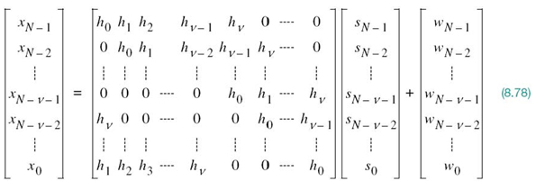
In a compact way, we may describe the discrete-time representation of the channel in the matrix form
where the transmitted symbol vector s, the channel noise vector w, and the received signal vector x are all N-by-1 vectors that are respectively defined as follows:
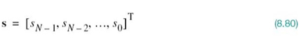
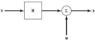
Figure 8.29 Discrete-time representation of multichannel data transmission system.
We may thus simply depict the discrete-time representation of the channel as in Figure 8.29 The N-by-N channel matrix H is itself defined by
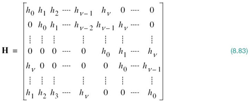
From the definition in (8.83), we readily see that the matrix H has the following structural composition:
Every row of the matrix is obtained by cyclically applying a right-shift to the previous row by one position, with the added proviso that the rightmost element of the previous row spills over in the shifting process to be “circulated” back to the leftmost element of the next row.
Accordingly, the matrix H is referred to as a circulant matrix.
Before proceeding further, it is befitting that we briefly review the DFT and its role in the spectral decomposition of the circulant matrix H.
Discrete Fourier Transform
Consider the N-by-1 vector x of (8.79). Let the DFT of the vector x be denoted by the N-by-1 vector
whose kth element is defined by
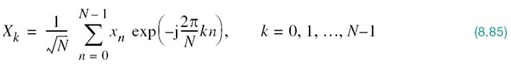
The exponential term exp(–j2Πkn/N) is the kernel of the DFT. Correspondingly, the IDFT (i.e., inverse DFT) of the N-by-1 vector X is defined by
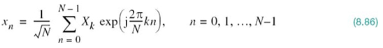
Equations (8.85) and (8.86) follow from discretizing the continuous-time Fourier transform both in time and frequency, as discussed in Chapter 2 with one difference: the DFT in(8.65) and its inverse in (8.66) have the same scaling factor, ![]() for the purpose of symmetry.
for the purpose of symmetry.
Although the DFT and IDFT appear to be similar in their mathematical formulations, their interpretations are different, as discussed previously in Chapter 2. As a reminder, we may interpret the DFT process described in (8.85) as a system of N complex heterodyning and averaging operations, as shown in Figure 2.32a. In the picture depicted in this part of the figure, heterodyning refers to the multiplication of the data sequence xn by one of N complex exponentials, exp(–j2Πkn/N). As such, (8.85) may be viewed as the analysis equation. For the interpretation of (8.86), we may view it as the synthesis equation: specifically, the complex Fourier coefficient Xk is weighted by one of N complex exponentials exp(–j2Πkn/N). At time n, the output xn is formed by summing the weighted complex Fourier coefficients, as shown in Figure 2.32b.
An important property of a circulant matrix, exemplified by the channel matrix H of (8.83), is that it permits the spectral decomposition defined by
where the superscript † denotes Hermitian transposition (i.e., the combination of complex conjugation and ordinary matrix transposition). Descriptions of the matrices Q and ⋀ are presented in the following in that order. The matrix Q is a square matrix defined in terms of the kernel of the N-point DFT as shown by
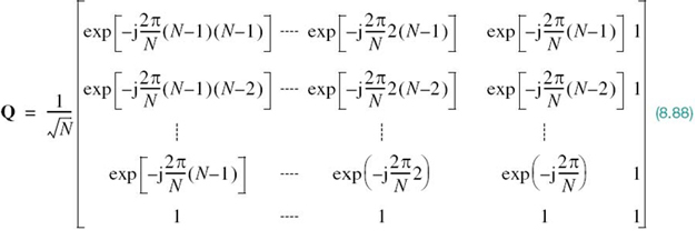
From this definition, we readily see that the klth element of the N-by-N matrix, Q, starting from the bottom right at k = 0 and l = 0 and counting up step-by-step, is
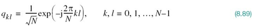
The matrix Q is an orthonormal matrix or unitary matrix, in the sense that it satisfies the condition
where I is the identity matrix. That is, the inverse matrix of Q is equal to the Hermitian transpose of Q.
The matrix ∧ in (8.87) is a diagonal matrix that contains the N DFT values of the sequence h0, h1,…,hν that characterize the channel. Denoting these transform values by λN – 1,…,λ1, λ0, respectively, we may express ∧ as
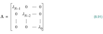
Note that λ used here are not to be confused with the Lagrange multipliers in Section 8.13.
From a system design objective, the DFT has established itself as one of the principal tools of digital signal processing by virtue of its efficient computation using the FFT algorithm, which was also described in Chapter 2. Computationally speaking, the FFT algorithm requires on the order of Nlog2N operations rather than the N2 operations for direct computation of the DFT. For efficient implementation of the FFT algorithm, we should choose the block length N to be an integer power of 2. The computational savings obtained by using the FFT algorithm are made possible by exploiting the special structure of the DFT defined in (8.85). Moreover, these savings become more substantial as we increase the data length N.
Frequency–Domain Description of the Channel
With this brief review of the DFT and its FFT implementations at hand, we are ready to resume our discussion of the DMT system. First, we define
where S is the frequency-domain vector representation of the transmitter output. Each element of the N-by-1 vector S may be viewed as a complex-valued point in a two-dimensional QAM signal constellation. Given the channel output vector x, we define its corresponding frequency-domain representation as
Using (8.87), (8.92), and (8.93), we may rewrite (8.79) in the equivalent form
Hence, using the equality of (8.90) in (8.94) we may reduce the vector to the simple form
where
In expanded (scalar) form, the matrix equation (8.95) reads as follows:
where the set of frequency-domain values ![]() is known for a prescribed channel. Note that Xk is a random variable and wk is a random variable sampled from a white Gaussian noise process.
is known for a prescribed channel. Note that Xk is a random variable and wk is a random variable sampled from a white Gaussian noise process.
For a channel with additive white noise, (8.97) leads us to make the following important statement:
The receiver of a DMT-based DSL is composed of a set of independent processors operating in parallel.
With the λk being all known, we may thus use the block of frequency-domain values ![]() to compute estimates of the corresponding transmitted block of frequency-domain values
to compute estimates of the corresponding transmitted block of frequency-domain values ![]() .
.
DFT-Based DMT System
Equations (8.95), (8.85), (8.86), and (8.97) provide the mathematical basis for the implementation of DMT using the DFT. Figure 8.30 illustrates the block diagram of the system derived from these equations, setting the stage for their practical roles:
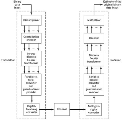
Figure 8.30 Block diagram of the DFT-based DMT system.
1. The transmitter consists of the following functional blocks:
- Demultiplexer, which converts the incoming serial data stream into parallel form.
- Constellation encoder, which maps the parallel data into N/2 multibit subchannels with each subchannel being represented by a QAM signal constellation. Bit allocation among the subchannels is also performed here in accordance with a loading algorithm.
- IDFT, which transforms the frequency-domain parallel data at the constellation encoder output into parallel time-domain data. For efficient implementation of the IDFT using the FFT algorithm, we need to choose N = 2k, where k is a positive integer.
- Parallel-to-serial converter, which converts the parallel time-domain data into serial form. Guard intervals stuffed with cyclic prefixes are inserted into the serial data on a periodic basis before conversion into analog form.
- Digital-to-analog converter (DAC), which converts the digital data into analog form ready for transmission over the channel.
Typically, the DAC includes a transmit filter. Accordingly, the time function h(t) in Figure 8.25 should be redefined as the combined impulse response of the cascade connection of the transmit filter and the channel.
2. The receiver performs the inverse operations of the transmitter, as described here:
- Analog-to-digital converter (ADC), which converts the analog channel output into digital form.
- Serial-to-parallel converter, which converts the resulting bit stream into parallel form. Before this conversion takes place, the guard intervals (cyclic prefixes) are removed.
- DFT, which transforms the time-domain parallel data into frequency-domain parallel data; as with the IDFT, the FFT algorithm is used to implement the DFT.
- Decoder, which uses the DFT output to compute estimates of the original multibit subchannel data supplied to the transmitter.
- Multiplexer, which combines the estimates so computed to produce a reconstruction of the transmitted serial data stream.
To sum up:
Thanks to the computationally efficient FFT algorithm, the DMT has established itself as the standard core technology for the design of asymmetric and very high bit-rate versions of the DSL by virtue of two important operational attributes: effective performance and efficient implementation.
Practical Applications of DMT-based DSL
An important application of DMT is in the transmission of data over two-way channels. Indeed, DMT has been standardized for use on ADSLs using twisted wire-pairs. In ADSL, for example, the DMT provides for the transmission of data downstream (i.e., from an ISP to a subscriber) at the rate of 1.544 Mbits/s and the simultaneous transmission of data upstream (i.e., from the subscriber to the ISP) at 160 kbits/s. This kind of data transmission capability is well suited for handling data-intensive applications such as video-on-demand.
DMT is also a core technology in implementing the asymmetric VDSLs, which differs from all other DSL transmission techniques because of its ability to deliver extremely high data rates. For example, a VDSL can provide data rates of 13 to 26 Mbits/s downstream and 2 to 3 MB/s upstream over twisted wire-pairs that emanate from an optical network unit and connect to the subscriber over distances of less than about 1 km. These high data rates allow the delivery of digital TV, super-fast Web surfing and file transfer, and virtual offices at home.
From a practical perspective, the use of DMT for implementing ADSL and VDSL provides a number of advantages:
- The ability of DMT to maximize the transmitted bit rate, which is provided by tailoring the distribution of information-bearing signals across the channel according to channel attenuation and noise conditions.
- Adaptivity to changing line conditions, which is realized by virtue of the fact that the channel is partitioned into a number of subchannels.
- Reduced sensitivity to impulse noise, which is achieved by spreading its energy over the many subchannels of the receiver. As the name implies, impulse noise is characterized by long, quiet intervals followed by narrow pulses of randomly varying amplitude. In an ADSL or VDSL environment, impulse noise arises due to switching transients coupled to twisted wire-pairs in the central office and to various electrical devices on the user’s premises.
- Effectively, employment of the DMT system eliminates the need for adaptive channel equalization.
8.16 Summary and Discussion
In this chapter devoted to data transmission over band-limited channels, two important aspects of this practical problem were discussed.
In the first part of the chapter, we assumed that the SNR at the channel input is large enough for the effect of channel noise to be ignored. Under this assumption, the issue of dealing with intersymbol interference was viewed as a signal design problem. That is, the overall pulse shape p(t) is configured in such a way that p(t) is zero at the sampling times nTb, where Tb is the reciprocal of the bit rate Rb. In so doing, the intersymbol interference is reduced to zero. Finding the pulse shape that satisfies this requirement is best handled in the frequency domain. The ideal solution is a “brick-wall” spectrum that is constant over the interval –W ≤ f ≤ W where W = 1/2Tb. Tb is the bit duration and W is called the Nyquist bandwidth. Unfortunately, this ideal pulse shape is impractical on two accounts: noncausal behavior and sensitivity to timing errors. To overcome these two practical difficulties, we proposed the use of an RC spectrum that rolls off gradually from a constant value over a prescribed band toward zero in a half-cosine-like manner on either side of the band. We finished this first part of the chapter by introducing the SRRC spectrum, where the overall pulse shaping is split equally between the transmitter and receiver; this latter form of signal design finds application in wireless communication.
Turning next to the second part of the chapter, we discussed another way of tackling data transmission over a wideband channel by applying the engineering principle of “divide and conquer.” Specifically, a telephone channel, using a twisted wire-pair, is partitioned into a large number of narrowband subchannels, such that each noisy subchannel can be handled by applying Shannon’s information-capacity law. Then, through a series of clever mathematical steps, the treatment of a difficult “discrete multicarrier transmission system” is modified into a new “DMT system.” Most importantly, by exploiting the computational efficiency of the FFT algorithm, practical implementation of the DMT assumes a well-structured transceiver (i.e., pair of transmitter and receiver) that is effective in performance and efficient in computational terms. Indeed, the DMT has established itself as the standard core technology for designing the asymmetric and very high bit-rate members of the digital subscriber line family. Moreover, the world-wide deployment of DSL technology has converted an ordinary telephone line into a broadband communication link, so much so that we may now view the PSTN as a broadband backbone data network. Most importantly, this analog-to-digital network conversion has made it possible to transmit data at rates in the megabits per second region, which is a truly a remarkable engineering achievement.
Problems
Nyquist’s Criterion
8.1 The NRZ pulse of Figure P8.1 may be viewed as a very crude form of a Nyquist pulse. Justify this statement by comparing the spectral characteristics of these two pulses.
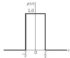
8.2 A binary PAM signal is to be transmitted over a baseband channel with an absolute maximum bandwidth of 75 kHz. The bit duration is 10. Find an RC spectrum that satisfies these requirements.
8.3 An analog signal is sampled, quantized, and encoded into a binary PCM. Specifications of the PCM signal include the following:
- Sampling rate, 8 kHz
- Number of representation levels, 64.
The PCM signal is transmitted over a baseband channel using discrete PAM. Determine the minimum bandwidth required for transmitting the PCM signal if each pulse is allowed to take on the following number of amplitude levels: 2, 4, or 8.
8.4 Consider a baseband binary PAM system that is designed to have an RC spectrum P(ƒ). The resulting pulse p(t) is defined in (8.25). How would this pulse be modified if the system is designed to have a linear phase response?
8.5 Determine the Nyquist pulse whose inverse Fourier transform is defined by the frequency function P(ƒ) defined in (8.26).
8.6 Continuing with the defining condition in Problem 8.5, namely
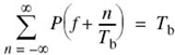
demonstrate that the Nyquist pulse p(t) with the narrowest bandwidth ![]() is described by the sinc function:
is described by the sinc function:
![]()
8.7 A pulse p(t) is said to be orthogonal under T-shifts if it satisfies the condition
![]()
where Tb is the bit duration. In other words, the pulse p(t) is uncorrelated with itself when it is shifted by any integer multiple of Tb. Show that this condition is satisfied by a Nyquist pulse.
8.8 Let P(ƒ) be an integrable function, the inverse Fourier transform of which is given by
![]()
and let Tb be given. The pulse p(t) so defined is a Nyquist pulse of bit duration Tb if, and only if, the Fourier transform P(ƒ) satisfies the condition
Using the Poisson sum formula described in Chapter 2, demonstrate the validity of this statement.
8.9 Let g(t) denote a function, the Fourier transform of which is denoted by G(ƒ). The pulse g(t) is orthogonal under T-shifts in that its Fourier transform G(ƒ) satisfies the condition
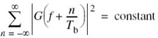
Show that this condition is satisfied by the SRRC shaping pulse.
Partial Response Signaling
8.10 The sinc pulse is the optimum Nyquist pulse, optimum in the sense it produces zero intersymbol interference occupying the minimum bandwidth possible W = 1/2Tb, where Tb is the bit duration. However, as discussed in Section 8.5, the sinc pulse is prone to timing errors; hence the preference for the RC spectrum that requires twice the minimum bandwidth, 2W.
In this problem, we explore a new pulse that achieves the minimum possible bandwidth W = 1/2Tb as the sinc pulse, but at the expense of a deterministic (i.e., controlled) intersymbol interference; being controllable, appropriate measures can be taken at the receiver to account for it.
This new pulse is denoted by g1(t), the Fourier transform of which is denoted by

a. Plot the magnitude and phase spectrum of G1(f).
b. Show that the pulse g1(t) is defined by
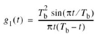
and therefore justify the statement that the tails of g1(t) decay as 1/|t|2, which is faster than the rate of decay 1/|t|, that characterizes the sinc pulse. Comment on this advantage of g1(t) over the sinc pulse.
c. Plot the waveform of g1(t) to demonstrate that g1(t) has only two distinguishable values at the sampling instants; hence the reference to g1(t) as a duobinary code.
d. Signaling over a band-limited channel with the use of a duobinary code is referred to partial-response signaling. Explain why.
8.11 In this problem, we explore another form of partial-response signaling based on the modified duobinary code. Let this second code be represented by the pulse g2(t) whose Fourier transform is defined by
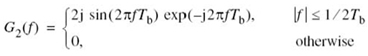
a. Plot the magnitude and phase spectra of G2(ƒ).
b. Show that the modified duobinary pulse is itself defined by
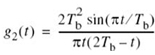
and therefore demonstrate that it has three distinguishable levels at the sampling instants.
c. What is a practical advantage of the modified duobinary code over the duobinary code in terms of transmission over a band-limited channel?
Multichannel Line Codes
8.12 Consider the passband basis functions defined in (8.56), where ϕ(t) is itself defined by (8.57). Demonstrate the validity of Properties 1, 2, and 3 of these passband basis functions.
8.13 The water-filling solution for the loading problem is defined by (8.73) subject to the constraint of (8.70). Using this pair of relations, formulate a recursive algorithm for computing the allocation of the transmit power P among the N subchannels. The algorithm should start with an initial total or sum noise-to-signal ratio NSR(i) = 0 for iteration i = 0, and the subchannels sorted in terms of those with the smallest power allocation to the largest.
8.14 The squared magnitude response of a linear channel, denoted by ![]() is shown in Figure P8.14. Assuming that the gap Г =1 and the noise variance σn2=1 for all subchannels, do the following:
is shown in Figure P8.14. Assuming that the gap Г =1 and the noise variance σn2=1 for all subchannels, do the following:
a.Derive the formulas for the optimum powers P1, P2, and P3, allocated to the three subchannels of frequency bands (0, W1), (W1, W2), and (W2, W).
b.Given that the total transmit power P = 10, l1 = 2/3, and l2 = 1/3, calculate the corresponding values of P1, P2, and P3.
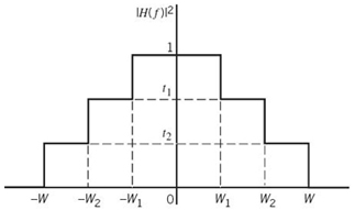
8.15 In this problem we explore the use of singular value decomposition (SVD) as an alternative to the DFT for vector coding. This approach avoids the need for a cyclic prefix, with the channel matrix being formulated as
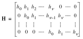
where the sequence h0, h1,…,hv denotes the sampled impulse response of the channel. The SVD of the matrix H is defined by
![]()
where U is an N-by-N unitary matrix and V is an (N + v)-by-(N + v) unitary matrix; that is,
![]()
where I is the identity matrix and the superscript ![]() denotes Hermitian transposition. The ∧ is an N-by-N diagonal matrix with singular values λn, n=1,2,…,N. The 0N, v is an N-by-v matrix of zeros.
denotes Hermitian transposition. The ∧ is an N-by-N diagonal matrix with singular values λn, n=1,2,…,N. The 0N, v is an N-by-v matrix of zeros.
a. Using this decomposition, show that the N subchannels resulting from the use of vector coding are mathematically described by
![]()
The Xn is an element of the matrix product ![]() , where x is the received signal (channel output) vector. An is the nth symbol an + jbn and Wn is a random variable due to channel noise.
, where x is the received signal (channel output) vector. An is the nth symbol an + jbn and Wn is a random variable due to channel noise.
b. Show that the SNR for vector coding as described herein is given by
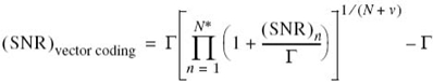
where ![]() is the number of channels for each of which the allocated transmit power is nonnegative, (SNR)n is the SNR of subchannel n, and Γ is a prescribed gap.
is the number of channels for each of which the allocated transmit power is nonnegative, (SNR)n is the SNR of subchannel n, and Γ is a prescribed gap.
c. As the block length N approaches infinity, the singular values approach the magnitudes of the channel Fourier transform. Using this result, comment on the relationship between vector coding and discrete multitone.
Computer Experiments
**8.16 In this computer-oriented problem, consisting of two parts, we demonstrate the effect of nonlinearity on eye patterns.
a. Consider a 4-ary PAM system, operating under idealized conditions: no channel noise and no ISI. the specifications are as follows:
Nyquist bandwidth, W = 0.5 Hz
Roll-off factor, α = 0.5
Symbol duration, T = 2Tb for M = 4 and Tb is the bit duration.
Compute the eye pattern for this noiseless PAM system.
b. Repeat the computation, this time assuming that the channel is nonlinear with the following input–output relationship:
![]()
where s(t) is the channel input and x(t) is the channel output (i.e., received signal); the a is a constant. Compute the eye pattern for the following three nonlinear conditions:
Hence, discuss how varying the constant a affects the shape of the eye pattern for the 4-ary PAM system.
Notes
1. The criterion described in (8.11) or (8.15) was first formulated by Nyquist in the study of telegraph transmission theory; the Nyquist (1928b) paper is a classic. In the literature, this criterion is referred to as Nyquist’s first criterion. In the 1928b paper, Nyquist described another method, referred to in the literature as Nyquist’s second criterion. The second method makes use of the instants of transition between unlike symbols in the received signal rather than centered samples. A discussion of the first and second criteria is presented in Bennett (1970: 78–92) and in the paper by Gibby and Smith (1965). A third criterion attributed to Nyquist is discussed in Sunde (1969); see also the papers by Pasupathy (1974) and Sayar and Pasupathy (1987).
2. The specifications described in Example 1 follow the book by Tranter et al. (2004).
3. The SRRC pulse shaping is discussed in Chennakeshu and Saulnier (1993) in the context of Π/4-shifted differential QPSK for digital cellular radio. It is also discussed in Anderson (2005: 27–29).
4. In a strict sense, an eye pattern that is completely open occupies the range from –1 to +1. On this basis, zero intersymbol interference would correspond to an ideal eye opening of 2. However, for two reasons, convenience of presentation and consistency with the literature, we have chosen an eye opening of unity to refer to the ideal condition of zero intersymbol interference.
5. For a detailed treatment of decision feedback equalizers, see the fifth edition of the classic book on Digital Communications by Proakis and Salehi (2008).
6. The idea of an ADSL is attributed to Lechleider (1989) in having had the insight that such an arrangement offers the possibility of more than doubling the information capacity of a symmetric arrangement.
7. For a detailed discussion of VDSL, see Chapter 7 of the book by Starr et al. (2003); see also the paper by Cioffi et al. (1999).
8. The method of Lagrange multipliers is discussed in Appendix D.