APPENDIX

F   Interleaving

Previous chapters of the book, going back to Chapter 5, have shown us how a digital wireless communication system can be separated by function into source-coding and channel-coding applications on the transmitting side and the corresponding inverse functions on the receiving side. In Chapter 6, we also learned how analog signals can be converted into a digital format. The motivation behind these techniques is to minimize the amount of information that has to be transmitted over a wireless channel. Such minimization has potential benefits in the allocation of two primary resources, namely transmit power and channel bandwidth, available to wireless communications:

1.  Reducing the amount of data that must be transmitted, which usually means that less power has to be consumed; power consumption is always a serious concern for mobile units that are typically battery operated.

2.  Reducing the spectral (or radio-frequency) resources, which are required for satisfactory performance; this reduction enables us to increase the number of users who can share the same but limited channel bandwidth.

Moreover, insofar as channel coding is concerned, forward error-correction (FEC) coding, discussed in Chapter 10, provides a powerful technique for transmitting information-bearing data reliably from a source to a sink across the wireless channel.

However, to obtain the maximum benefit from FEC coding in wireless communications, we require an additional technique known as interleaving.¹ The need for this new technique is justified on the grounds that, in light of the material presented in Chapter 9, we know that wireless channels have memory due to multipath fading that results from the arrival of signals at the receiver via multiple propagation paths of different lengths. Of particular concern is fast fading, which arises out of reflections from objects in the local vicinity of the transmitter, the receiver, or both. The term fast refers to the speed of fluctuations in the received signal due to these reflections, relative to the speeds of other propagation phenomena. Compared with transmit data rates, even fast fading can be relatively slow. That is, fast fading can be approximately constant over a number of transmission symbols, depending upon the data transmission speed and the mobile unit’s velocity. Consequently, fast fading may be viewed as a time-correlated form of channel impairment, the presence of which results in statistical dependence among continuous (sets of) symbol transmissions. That is, instead of being isolated events, transmission errors due to fast fading tend to occur in bursts.

Now, most FEC channel codes are designed to deal with a limited number of bit errors, assumed to be randomly distributed and statistically independent from one bit to the next. To be specific, in Section 10.8 on convolutional decoding, we indicated that the Viterbi algorithm, as powerful as it is, will fail if there are d_free/2 closely spaced bit errors in the received signal, where d_free is the free distance of the convolutional code. Accordingly, in the design of a reliable wireless communication system, we are confronted with two conflicting phenomena:

• a wireless channel that produces bursts of correlated bit errors;
• a convolutional decoder that cannot handle error bursts.

Interleaving is an indispensable technique for resolving these two conflicting phenomena. First and foremost, however, it is important to note that for interleaving we do not need the exact statistical characterization of the wireless channel. Rather, we only require knowledge of the coherence time for fast fading, which is approximately given by (see (9.46))

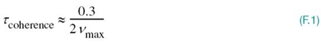
where V_max is the maximum Doppler shift. Consequently, we would expect an error burst to occupy typically a time duration equal to τ_coherence. To deal with bad situations of this kind in wireless communications, we do two things:

• An interleaver (i.e., a device that performs interleaving) is used to randomize the order of encoded bits after the channel encoder in the transmitter.
• A de-interleaver (i.e., a device that performs de-interleaving) is used to undo the randomization before the data reach the channel decoder in the receiver.

Interleaving has the net effect of breaking up any error bursts that may occur during the course of data transmission over the wireless channel and spreading them over the duration of operation of the interleaver. In so doing, the likelihood of a correctable received sequence is significantly improved. In the transmitter, the interleaver is placed after the channel encoder; in the receiver, the de-interleaver is placed before the channel decoder.

Three types of interleaving are commonly used in practice, and are discussed next.

F.1   Block Interleaving

In basic terms, a classical block interleaver acts as a memory buffer, as shown in Figure F.1. Data are written into this N × L rectangular array from the channel encoder in column fashion. Once the array is filled, it is read out in row fashion and its contents are sent to the transmitter. At the receiver, the inverse operation is performed: the contents of the array in the receiver are written row-wise with data; once the array is filled, it is read out column-wise into the decoder. Note that the (N, L) interleaver and de-interleaver described herein are both periodic with the fundamental period T = NL.

Suppose the correlation time or error-burst-length time corresponds to L received bits. Then, at the receiver, we expect that the effect of an error burst would corrupt the equivalent of one row of the de-interleaver block. However, since the de-interleaver block is read columnwise, all of these “bad” bits would be separated by N − 1 “good” bits when the burst is read into the decoder. If N is greater than the constraint length of the convolutional code being employed, then the Viterbi decoder will correct all of the errors in the error burst.

In practice, owing to the frequency of error bursts and the presence of other errors caused by channel noise, the interleaver should ideally be made as large as possible. However, an interleaver introduces delay into the transmission of the message signal, in that we must fill the N × L array before it can be transmitted. This is an issue of particular concern in real-time applications such as voice, because it limits the usable block size of the interleaver and necessitates a compromise solution.

Figure F.1 Block interleaver structure. (a) Data “read in.”(b) Data “read out.”

EXAMPLE 1   Interleaving

Figure F.2a depicts an original sequence of encoded words, with each word consisting of five symbols. Figure F.2b depicts the interleaved version of the encoded sequence, with the symbols shown in reordered positions. An error burst occupying five symbols, caused by channel impairment, is also shown alongside Figure F.2b. Note that the manner in which the encoded symbols are reordered by the interleaver is the same from one word to the next.

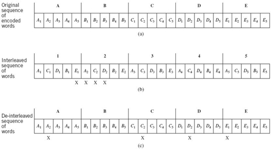
Figure F.2 Interleaving example. (a) Original sequence. (b) Interleaved sequence. (c) De-interleaved sequence.

On de-interleaving in the receiver, the scrambling of symbols is undone, yielding a sequence that resembles the original sequence of encoded symbols, as shown in Figure F.2c. This figure also includes the new positions of the transmission errors. The important point to note here is that the error burst is dispersed as a result of de-interleaving.

This example teaches us the following:

1.  The burst of transmission errors is only acted upon by the de-interleaver.

2.  Insofar as the encoded symbols that are received are error free, the de-interleaver cancels the scrambling action of the interleaver.

F.2 Convolutional Interleaving

The block diagram of a convolutional interleaver/de-interleaver is shown in Figure F.3. Defining the period

the interleaver is referred to as an (L × N) convolutional interleaver, which has properties similar to those of the (L × N) block interleaver.

The sequence of encoded bits to be interleaved in the transmitter is arranged in blocks of L bits. For each block, the encoded bits are sequentially shifted into and out of a bank of N registers by means of two synchronized input and output commutators. The interleaver, depicted in Figure F.3a, is structured as follows:

1.  The zeroth shift register provides no storage; that is, the incoming encoded symbol is transmitted immediately.

2.  Each successive shift register provides a storage capacity of L symbols more than the preceding shift register.

3.  Each shift register is visited regularly on a periodic basis.

With each new encoded symbol, the commutators switch to a new shift register. The new symbol is shifted into the register and the oldest symbol stored in that register is shifted out. After finishing with the (N − 1)th shift register (i.e., the last register), the commutators return to the zeroth shift register. Thus, the switching/shifting procedure is repeated periodically on a regular basis.

The de-interleaver in the receiver also uses N shift registers and a pair of input/output commutators that are synchronized with those in the interleaver. Note, however, the shift registers are stacked in the reverse order to those in the interleaver, as shown in Figure F.3b. The net result is that the de-interleaver in the receiver performs the inverse operation to interleaving in the transmitter, and so it should.

An advantage of convolutional over block interleaving is that in convolutional interleaving the total end-to-end delay is L(N − 1) symbols and the memory requirement is L(N − 1)/2 in both the interleaver and de-interleaver, which are one-half of the corresponding values in a block interleaver/de-interleaver for a similar level of interleaving.

The description of the convolutional interleaver/de-interleaver in Figure F.3b is presented in terms of shift registers. The actual implementation of the system can also be accomplished with a random access memory unit in place of shift registers. This alternative implementation simply requires that access to the memory units be appropriately controlled.

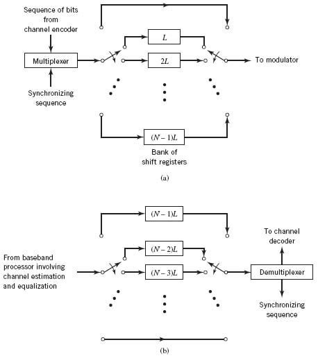
Figure F.3 (a) Convolutional interleaver. (b) Convolutional de-interleaver.

F.3   Random Interleaving

In a random interleaver, a block of N input bits is written into the interleaver in the order in which they are received, but they are read out in a random manner. Typically, the permutation of the input bits is defined by a uniform distribution. Let π(i) denote the permuter location of the ith input bit, where i = 1,2,…N. The set of integers denoted by , defining the order in which the stored input bits are read out of the interleaver, is generated according to the following two-step algorithm:

1.  Choose an integer i₁ from the uniformly distributed set ={1,2,…,N}, with the probability of choosing i₁ being p(i₁) = 1/N. The chosen integer i₁ is set to be π(i).

2.  For k > 1, choose an integer i_k from the uniformly distributed set

with the probability of choosing i_k being p(i_k) = 1/(N − k +1). The chosen integer i_k is set to be π(k). Note that the size of the set _k is progressively reduced for k > 1. When k = N, we are left with a single integer i_N, in which case i_N is set to be π(N).

To be of practical use in communications, random interleavers are configured to be pseudo-random, meaning that within a block of N input bits the permutation is random as described above, but the permutation order is exactly the same from one block to the next. Accordingly, pseudo-random interleavers are designed off-line; they are of particular interest in the construction of turbo codes, discussed in Chapter 10.

       Notes

1. Interleaving of both the block and convolutional types is discussed in some detail in Clark and Cain (1981) and in lesser detail in Sklar (2001). For a treatment of interleaving viewed from the perspective of turbo codes, see the book (Vucetic and Yuan, 2000).