APPENDIX

D  Method of Lagrange Multipliers

D.1  Optimization Involving a Single Equality Constraint

Consider the minimization of a real-valued function ƒ(w) that is a quadratic function of a parameter vector w, subject to the constraint

where s is a prescribed vector and g is a complex constant; the superscript denotes Hermitian transposition. We may redefine the constraint by introducing a new function c(w) that is linear in w, as shown by

In general, the vectors w and s and the function c(w) are all complex. For example, in a beamforming application, the vector w represents a set of complex weights applied to the individual sensor outputs and s represents a steering vector whose elements are defined by a prescribed “look” direction; the function ƒ(w) to be minimized represents the mean-square value of the overall beamformer output. In a harmonic retrieval application, for another example, w represents the tap-weight vector of an FIR filter and s represents a sinusoidal vector whose elements are determined by the angular frequency of a complex sinusoid contained in the filter input; the function ƒ(w) represents the mean-square value of the filter output. In any event, assuming that the issue is one of minimization, we may state the constrained optimization problem as follows:

The method of Lagrange multipliers converts the problem of constrained minimization just described into one of unconstrained minimization by the introduction of Lagrange multipliers. First, we use the real function ƒ(w) and the complex constraint function c(w) to define a new real-valued function

where λ₁ and λ₂ are real Lagrange multipliers and

Now we define a complex Lagrange multiplier:

The Re[∙] and Im[∙] in (D.4) and (D.5) denote real and imaginary operators, respectively. We may then rewrite (D.4) in the form

where the asterisk denotes complex conjugation.

Next, we minimize the function h(w) with respect to the vector w. To do this, we set the conjugate derivative ∂h/ (∂w^∗) equal to the null vector:

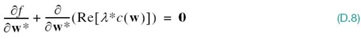
The system of simultaneous equations consisting of (D.8) and the original constraint given in (D.2) defines the optimum solutions for the vector w and the Lagrange multiplier λ. We call (D.8) the adjoint equation and (D.2) the primal equation (Dorny, 1975).