APPENDIX

E  Information Capacity of MIMO Channels

The topic of multiple-input multiple-output (MIMO) links for wireless communications was discussed in Chapter 9 on signaling over fading channels. To get a measure of the transmission efficiency of MIMO links therein, we resorted to the notion of outage capacity, which is naturally of practical interest. However, in light of its mathematical sophistication, we deferred discussion of the information capacity of MIMO links rooted in Shannon’s information theory to this appendix.

To be specific, in this appendix we discuss two different aspects of information capacity:

1. The channel state is known to the receiver but not the transmitter;

2. The channel state is known to both the receiver and the transmitter.

The discussion will proceed in this order.

E.1   Log-Det Capacity Formula of MIMO Channels

Consider a communication channel with multiple antennas.¹ Let the N_t-by-1 vector s denote the transmitted signal vector and the N_r-by-1 vector x denote the received signal vector. These two vectors are related by the input−output relation of the channel:

where H is the channel matrix of the link and w is the additive channel noise vector. The vectors s, w, and x are realizations of the random vectors S, W, and X, respectively.

In what follows in this appendix, the following assumptions are made:

1. The channel is stationary and ergodic.

2. The channel matrix H is made up of iid Gaussian elements.

3. The transmitted signal vector s has zero mean and correlation matrix R_s.

4. The additive channel noise vector w has zero mean and correlation matrix R_w.

5. Both s and w are governed by Gaussian distributions.

In this section, we also assume that the channel state H is known to the receiver but not the transmitter. With both H and x unknown to the transmitter, the primary issue of interest is to determine I(s;x, H), which denotes the mutual information between the transmitted signal vector s and both the received signal vector x and the channel matrix H. Extending the definition of mutual information introduced in Chapter 5 to the problem at hand, we write

where and are the respective spaces pertaining to the random vectors S and X and matrix H.

Using the definition of a joint probability density function (pdf) as the product of a conditional pdf and an ordinary pdf, we write

We may therefore rewrite (E.2) in the equivalent form

where the expectation is with respect to the channel matrix H and

is the conditional mutual information between the transmitted signal vector s and received signal vector x, given the channel matrix H. However, by assumption, the channel state is unknown to the transmitter. Therefore, it follows that, insofar as the receiver is concerned, I(s;x∣H) is a random vector; hence the expectation with respect to H in (E.3). The quantity resulting from this expectation is therefore deterministic, defining the mutual information jointly between the transmitted signal vector s and both the received signal vector x and channel matrix H. The result so obtained is indeed consistent with what we know about the notion of joint mutual information.

Next, applying the vector form of the first line in (5.81) to the mutual information I(s;x∣H), we have

where h(x∣H) is the conditional differential entropy of the channel output x given H, and h(x∣s, H) is the conditional differential entropy of x, given both s and H. Both of these entropies are random quantities, because they both depend on H.

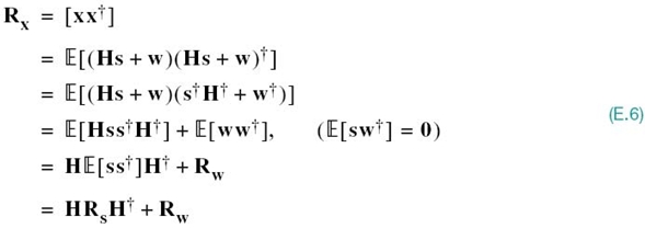
To proceed further, we now invoke the assumed Gaussianity of both s and H, in which case x also assumes a Gaussian description. Under these circumstances, we may use the result of Problem 5.32 to express the entropy of the received signal x of dimension N_r, given H, as

where R_x is the correlation matrix of x and det(R_x) is its determinant. Recognizing that the transmitted signal vector s and channel noise vector w are independent of each other, we find from (E.1) that the correlation matrix of the received signal vector x is given by

where denotes Hermitian transposition,

is the correlation matrix of the transmitted signal vector s, and

is the correlation matrix of the channel noise vector w. Hence, using (E.6) in (E.5), we get

where N_r is the number of elements in the receiving antenna. Next, we note that since the vectors s and w are independent and the sum of w plus Hs equals x as indicated in (E.1), then the conditional differential entropy of x, given both s and H, is simply equal to the differential entropy of the additive channel noise vector w; that is,

The differential entropy h(w) is given by (see Problem 5.32)

Thus, using (E.9), (E.10), and (E.11) in (E.4), we get

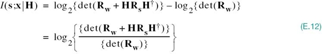
As remarked previously, the conditional mutual information I(s;x∣H) is a random variable. Hence, using (E.12) in (E.3), we finally formulate the ergodic capacity of the MIMO link as the expectation

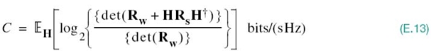
which is subject to the constraint

where P is constant transmit power and tr[∙] denotes the trace operator, which extracts the sum of the diagonal elements of the enclosed matrix.

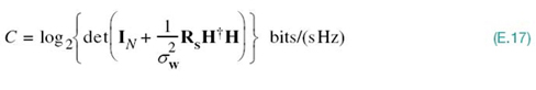
Equation (E.13) is the desired log-det formula for the ergodic capacity of the MIMO link. This formula is of general applicability, in that correlations among the elements of the transmitted signal vector s and among those of the channel noise vector w are permitted. However, the assumptions made in its derivation involve the Gaussianity of s, H, and w.

E.2   MIMO Capacity for Channel Known at the Transmitter

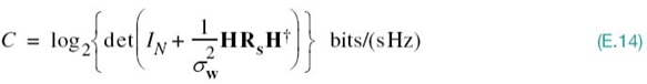
The log-det formula of (E.13) for the ergodic capacity of a MIMO flat-fading channel assumes that the channel state is only known at the receiver. What if the channel state is also known perfectly at the transmitter? Then the channel state becomes known to the entire system, which means that we may treat the channel matrix H as a constant. Hence, unlike the partially known case treated in Section E.1, there is no longer the need for invoking the expectation operator in formulating the log-det capacity. Rather, the problem becomes one of constructing the optimal R_s (i.e., the correlation matrix of the transmitted signal vector s) that maximizes the ergodic capacity. To simplify the construction procedure, we consider a MIMO channel for which the number of elements in the receiving antenna N_r and the number of elements in the transmitting antenna N_t have a common value, denoted by N.

Accordingly, using the assumption of additive white Gaussian noise with variance in the log-det capacity formula of (E.13), we get

We can now formally postulate the optimization problem at hand as follows:

Maximize the ergodic capacity C of (E.14) with respect to the correlation matrix R_s, subject to two constraints, expressed as

1. Nonnegative definite Rs, which is a necessary requirement for a correlation matrix.

2. Global power constraint

where P is the total transmit power.

To proceed with construction of the optimal R_s, we first use the determinant identity:

Application of this identity to (E.14) yields

Diagonalizing the matrix product HH by invoking the eigendecomposition of a Hermitian matrix, we write

where Λ is a diagonal matrix made up of the eigenvalues of, HH and U is a unitary matrix whose columns are the associated eigenvectors.² We may therefore rewrite (E.18) in the equivalent form

where by definition we have used the fact that the matrix product is equal to the identity matrix. Substituting (E.18) into (E.17), we get

Next, applying the determinant identity of (E.16) to the formula, we get

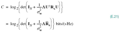
where

Note that the transformed correlation matrix is nonnegative definite. Since = I, we also have

where, in the second line, we used the equality tr[AB] = tr[BA]. It follows, therefore, that maximization of the ergodic capacity of (E.21) can be carried out equally well over the transformed correlation matrix .

One other important point to note is that any nonnegative definite matrix A satisfies the Hadamard inequality

where the a_kk are the diagonal elements of matrix A. Hence, applying this inequality to the determinent term in (E.21), we may write

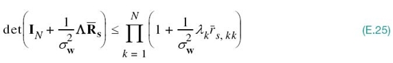
where λ_k is the kth eigenvalue of the matrix product and is the kth diagonal element of the transformed matrix . Equation (E.25) holds only when is a diagonal matrix, which is the very condition that maximizes the ergodic capacity C.

To proceed further, we now use (E.21) and (E.25) with the equality sign to express the ergodic capacity as

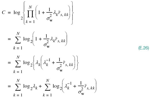
where only the second sum term is clearly adjustable through . We may therefore reformulate the optimization problem at hand as follows:

Given the set of eigenvalues pertaining to the matrix product , determine the optimal set of autocorelations that maximizes the summation

subject to the constraint

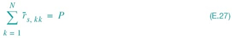
The global power constraint of (E.27) follows from (E.23) and the trace definition of a trace:

Water-Filling Interpretation of (E.26)

The solution to the reformulated optimization problem that was initiated after (E.14) may be determined through the discrete spatial version of the water-filling procedure, which is described in Chapter 5. Effectively, the solution to the water-filling problem says that, in a multiple-channel scenario, we transmit more signal power in the better channels and less signal power in the poorer channels. To be specific, imagine a vessel whose bottom is defined by the set of N dimensionless discrete levels

and pour “water” into the vessel in an amount corresponding to the total transmit power P. The power P is optimally divided among the N eigenmodes of the MIMO link in accordance with their corresponding “water levels” in the vessel, as illustrated in Figure E.1 for a MIMO link with N = 6. The “water-fill level, ” denoted by the dimensionless parameter μ and indicated by the dashed line in the figure, is chosen to satisfy the constraint of (E.27). 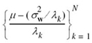On the basis of the spatially discrete water-filling picture portrayed in Figure E.1, we may now finally postulate the optimal to be

The superscript “+” applied to the right parenthesis in (E.29) signifies retaining only those terms in the right-hand side of the equation that are positive (i.e., the terms that pertain to those eigenmodes of the MIMO link for which the water levels lie below the constant μ).

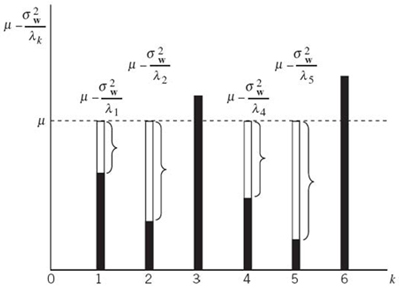
Figure E.1 Water-filling interpretation of the optimization procedure.

We may thus finally state that if the channel matrix H is known to both the transmitter and the receiver of a MIMO link with N_r = N_t = N, then the maximum value of the capacity of the MIMO link is defined by

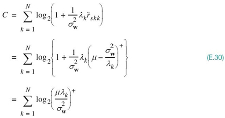
where, as stated previously, the constant μ is chosen to satisfy the global power constraint of (E.27).

       Notes

1. The first detailed derivation of the log-det capacity formula for a stationary MIMO channel was presented by Telatar in an AT&T technical memorandum published in 1995 and republished as a journal paper (Telatar, 1999).

2. Given a complex-valued matrix A, the eigendecomposition of A is defined by .