APPENDIX

A  Advanced Probabilistic Models

In the study of digital communications presented in preceding chapters, the Gaussian, Rayleigh, and Rician distributions featured in the formulation of probabilistic models in varying degrees. In this appendix we describe three relatively advanced distributions:

• the chi distribution;
• the log-normal distribution;
• the Nakagami distribution.

The chi distribution is featured in the study of diversity-on-receive techniques in Chapter 9 on signaling across fading channels. Just as importantly, the log-normal distribution was mentioned in passing in the context of shadowing in wireless communications, also in Chapter 9. The Nakagami distribution is the most advanced of all the three:

• it includes the Rayleigh distribution as a special case;
• its shape is similar to the Rician distribution;
• it is flexible in its applicability.

A.1   The Chi-Square Distribution

A chi-square χ² distributed random variable is produced, for example, when a Gaussian random variable is passed through a squaring device. Viewed in this manner, there are two kinds of χ² distributions:

1.  Central χ² distribution, which is produced when the Gaussian random variable has zero mean.

2.  Noncentral χ² distribution, which is produced when the Gaussian random variable has a nonzero mean.

In this appendix, we will discuss only the central form of the distribution.

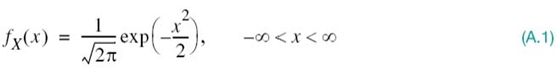
Consider, then, a standard Gaussian random variable X, which has zero mean and unit variance, as shown by

Let the variable X be applied to a square-law device, producing a new random variable Y, whose sample value is defined by

or, equivalently,

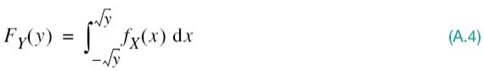
The cumulative distribution function of the random variable Y produced at the output of the square-law device is therefore defined by

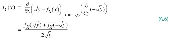
Differentiating F_Y(y) with respect to y yields the probability density function (pdf):

Substituting (A.1) into (A.5), we get

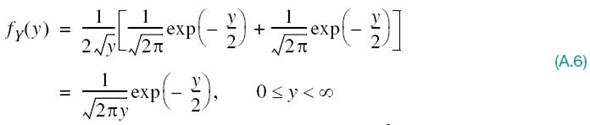
The distribution described in (A.6) is called the chi-square (χ²) distribution with one degree of freedom.

The first two moments of Y are given by

and its variance is

Note, however, that these values are based on the standard Gaussian distribution with zero mean and unit variance. For the general case of an ordinary Gaussian distribution with zero mean and variance σ², the mean, mean-square value, and variance of the X² random variable Y are, respectively, as follows:

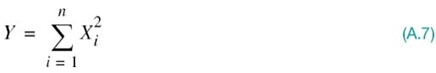
In its most general setting, derivation of the chi-square distribution follows from a set of iid random variables denoted by , on the basis of which a new random variable is defined as follows:

On this basis, the pdf of the random variable Y is defined by

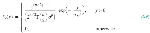
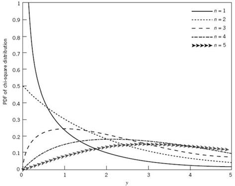
Figure A.1 The chi-square distribution for varying order n.

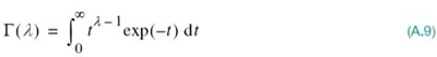
where Γ (λ) is Euler’s gamma function, defined by (Abramowitz and Stegun, 1965)

As such, the random variable Y is said to have the chi-square distribution of order n. When n = 1, Γ (1/2) = , and we get the special case described in (A.6); this special case of the χ² distribution is also referred to as the one-sided exponential distribution. Figure A.1 plots the χ² distribution for varying orders: n = 1, 2, 3, 4, 5.

A.2   The Log-Normal Distribution

To proceed next with the log-normal distribution, let X and Y be two random variables that are related to each other through the logarithmic transformation

where ln is the natural logarithm. Conversely, we have

In light of this logarithmic transformation, the random variable X is said to be log-normally distributed if the other random variable Y is normally (i.e., Gaussian) distributed.

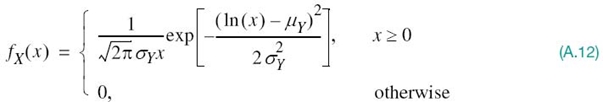
Assuming that the Gaussian-distributed Y has nonzero mean μ_Y and variance , then a straightforward transformation based on (A.11) yields the log-normal distribution:

By the same token, a probability model based on the log-normal distribution of (A.12) is called the log-normal model.

Unlike the chi-square distribution, the log-normal distribution has two adjustable parameters of its own, the nonzero mean μ_Y and variance , both of which are inherited from the Gaussian distributed random variable Y. Note also that the mean and variance of the log-normally distributed random variable X, represented by the sample value x in (A.12), are respectively different from the exponential functions of μ_Y and .

As already noted, the log-normal distribution of (A.12) is derived via the logarithmic transformation of a Gaussian-distribution. Recognizing that power plays a key role in the study of communications, there is special merit in introducing a new random variable related to X:

which is measured in decibels. Conversely, x is expressed in terms of z as follows:

Hence, using (A.14) in (A.13), we get

where the constant is

Equation (A.15) shows that both Y and Z are Gaussian distributed, differing by the scaling factor c.

Accordingly, the mean and variance of the Gaussian-distributed random variable Z are respectively defined by

Equivalently, we may write

To visualize the log-normal distribution defined in (A.12), we propose to proceed as follows:¹

1. The mean μ_Y is maintained at the constant value, μ_Y = 0 dB.

2. The standard deviation σ_Y (that is, the square root of the variance ) is assigned three different values: σ_Y = 1, 5, 10 dB.

With decibel as the logarithmic measure of interest, the new variable x in the log-normal distribution of (A.12) is also measured in decibels. Thus, using the assigned values of μ_Y and σ_Y under points (1) and (2) in (A.12), we get the plots displayed in Figure A.2.

Examining Figure A.2, we make two observations that are of particular interest:

1. The log-normal distribution exhibits long tails for σ_Z ≥ 6 dB; hence its appropriateness as a model for the shadow-fading phenomenon in wireless communications. From a practical perspective, a standard deviation lying in the range 6 ≤ σ_Z ≤ 8 dB is typical for shadowing, in which case we see that the distribution of Figure A.2 is quite asymmetric with a small “modal” value. In other words, 6 ≤ σ_Z ≤ 8 dB is the modeor the most likely range of shadowing.

2. When the standard deviation σ_Z is reduced below this range, the log-normal distribution tends to become more symmetric and, therefore, Gaussian, centered roughly around x = 1 dB.

Useful Properties of the Log-Normal Distribution

Over and above having the characteristic of long tails, the log-normal distribution has two other useful properties:²

PROPERTY 1  The product (or quotient) of log-normal variables is log-normal.

This property follows from the fact that the exponents of the random variable Y or Z add (or subtract). Since the exponents are Gaussian distributed, they remain Gaussian after the addition (or subtraction); hence the validity of Property 1.

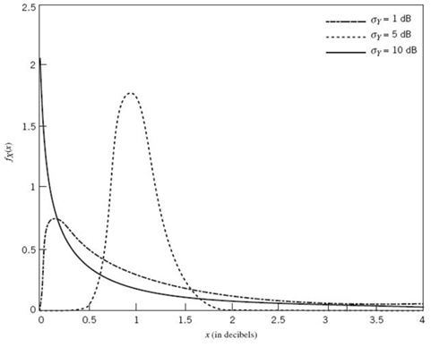
Figure A.2 The log-normal distribution.

As a corollary to this property, we may also state:

The amplitude and power of a log-normal random variable are both log-normal.

PROPERTY 2  The product of a large number of iid random variables is asymptotically log-normal.

This property is the counterpart of the central limit theorem, involving the addition of a large number of iid random variables. The reason for this second property is rather obvious for two reasons:

• First, the example of the random variables involved in forming the product add.
• Second, applying the central limit theorem to the addition of the example, the result asymptotically converges to a Gaussian distribution; hence the validity of Property 2.

A.3   The Nakagami Distribution

As different as the distributions covered until this point are, namely the Rayleigh and Rician distributions derived in Chapter 4, as well as the chi-square and log-normal distributions derived in this appendix, all four of them share a common factor:

They are derived from the Gaussian distribution through respective transformations.

In the last part of this appendix we describe another distribution, namely the Nakagami distribution, which is different from all the others in the following sense:

Through the use of simulation, the Nakagami distribution can be fitted directly to real-life data.

Indeed, it is for this important reason (and a few others that will be discussed) that the Nakagami distribution is commonly used as a model for wireless communications.

To be specific, a random variable X whose pdf is described by the equation

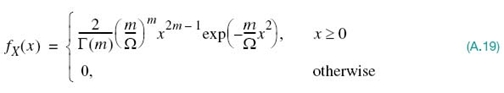
is said to have the Nakagami-m distribution. The random variable X is itself referred to as a Nakagami-distributed random variable (Nakagami, 1960).

The two parameters that characterize this distribution are defined as follows:

1. The parameter Ω, which is the mean-square value of the random variable X; that is,

2. The second parameter, m, called the fading figure, is defined by the ratio:

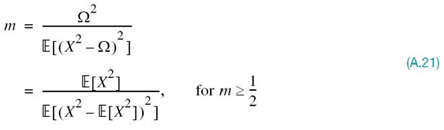
Note the restriction that is placed on m for (A.21) to hold. Close examination of the definitions embodied in (A.20) and (A.21) reveals that the statistical characterization of the fading figure m involves two moments:

• the mean-square value of the random variable X in the numerator and
• the variance of the squared random variable X² in the denominator.

It follows, therefore, that the fading figure m is dimensionless.

For visualization, the Nakagami-m distribution is plotted in Figure A.3 for varying values of m. Two observations from these plots are noteworthy:

1. For m = 1/2, the Nakagami-m distribution reduces to the Rayleigh distribution; in other words:

The Rayleigh distribution is a special case of the Nakagami distribution.

2. The Nakagami and Rician distributions have a similar shape.

To elaborate on point 2, for m > 1 we find that the fading figure m can be computed from the dimensionless Rice factor K (discussed in Chapter 4), as shown in (Stüber, 1996):

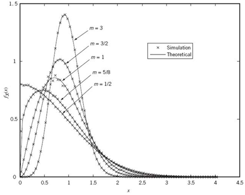
Figure A.3 The Nakagami-m distribution, presenting theoretical and simulation results for varying fading figure m.

Conversely,

A cautionary note is in order, however. Although the Nakagami-m and Rician distributions appear to have good agreement insofar as their shapes are concerned, they have different slopes at the origin, x = 0; this difference has a significant impact on the achievable diversity, with the advantage residing in the Nakagami distribution (Molisch, 2011).

From a practical perspective, the Nakagami-m distribution has the following attributes, in accordance with (A.20) and (A.21):

The two parameters, Ω and m, lend themselves to computation from experimentally measured data in a relatively straightforward manner.

This succinct statement re-emphasizes the point we made at the beginning of this subsection:

Through the use of simulation, real-life data can be fitted into the Nakagami distribution.

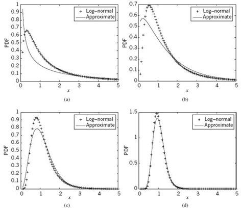
Figure A.4 A set of sample functions of log-normal distribution and its approximation with the Nakagami distribution as the fading figure m is increased.

Indeed, with this important point in mind, the plots presented in Figure A.3 actually include points (denoted by crosses) that pertain to an arbitrarily selected wireless data.³

Figure A.4 provides further demonstration of the inherent flexibility of the Nakagami-m distribution in approximating the log-normal distribution. It is clearly shown that the approximation gets gradually better as the fading figure m is increased.

It is not surprising, therefore, to find that the Nakagami-m distribution outperforms the Rayleigh and Rician distributions, particularly so in urban wireless communication environments.⁴

       Notes

1. The visualization procedure described herein for the log-normal distribution follows Cavers (2000).

Two other procedures for visualizing the log-normal distribution are described in the literature, as summarized here:

• In Proakis and Salehi (2008), the standard deviation σ_Y = 1 and the mean μ_Y are varied, with both μ_Y and σ_Y measured in volts.
• In Goldstein (2005), a new random variable Ψ defined as the ratio of transmit-to-receive power, is used in place of x, and a new formula for the log-normal distribution is derived. In so doing, the use of power measured in decibels plays a prominent role in a new formulation of the log-normal distribution. However, this new formulation takes values for 0 ≤ ψ < ∞, which raises a physically unacceptable scenario; specifically, for ψ < 1, the receive-power assumes a value greater than the transmit-power.
• Fortunately, the probability of this unacceptable scenario arising is very small, provided that the mean μ_ψ, expressed in decibels, is positive and large. It is thus claimed that the log-normal model based on the random variable ψ captures the underlying physical model very accurately when the mean μ_ψ is very large compared to 0 dB.

2. The properties of the log-normal distribution described herein follow Cavers (2000).

3. The procedure used to compute the simulated points in the plots presented in Figure A.3 follows Matthaiou and Laurenson (2007).

4. This note provides additional noteworthy material on the Nakagami-mdistribution. In Turin et al. (1972) and Suzuki (1977), it is demonstrated that the Nakagami-m distribution provides the best statistical fit to measured data in urban wireless environments.

Two other papers of interest are Braun and Dersch (1991), in which a physical interpretation of the Nakagami-m distribution is presented, and Abdi et al., (2000), in which the statistical characteristics of the Nakagami and Rician distributions are summarized.

Moreover, there are three other papers on the Nakagami distribution that deserve attention. Given a set of real-life fading-channel data, various papers have been published on how to estimate the parameter m in the Nakagami model. In Zhang (2002), numerical results are presented to show that none of the previously published results exceed the classical one by Greenwood and Durand (1960). The correlated Rayleigh fading lends itself readily to simulate a fading channel by virtue of its relationship to a complex Gaussian process. Unfortunately, this is not so with the Nakagami distribution. In Zhang (2000), a decomposition technique is described for the efficient generation of a correlated Nakagami fading channel.

In Zhang (2003), a generic correlated Nakagami-m model is described using a multiple joint characteristic function, which allows for an arbitrary covariance matrix and distinct real fading parameters.