CHAPTER

6

Conversion of Analog Waveforms into Coded Pulses

6.1    Introduction

In continuous-wave (CW) modulation, which was studied briefly in Chapter 2, some parameter of a sinusoidal carrier wave is varied continuously in accordance with the message signal. This is in direct contrast to pulse modulation, which we study in this chapter. In pulse modulation, some parameter of a pulse train is varied in accordance with the message signal. On this basis, we may distinguish two families of pulse modulation:

1. Analog pulse modulation, in which a periodic pulse train is used as the carrier wave and some characteristic feature of each pulse (e.g., amplitude, duration, or position) is varied in a continuous manner in accordance with the corresponding sample value of the message signal. Thus, in analog pulse modulation, information is transmitted basically in analog form but the transmission takes place at discrete times.

2. Digital pulse modulation, in which the message signal is represented in a form that is discrete in both time and amplitude, thereby permitting transmission of the message in digital form as a sequence of coded pulses; this form of signal transmission has no CW counterpart.

The use of coded pulses for the transmission of analog information-bearing signals represents a basic ingredient in digital communications. In this chapter, we focus attention on digital pulse modulation, which, in basic terms, is described as the conversion of analog waveforms into coded pulses. As such, the conversion may be viewed as the transition from analog to digital communications.

Three different kinds of digital pulse modulation are studied in the chapter:

1. Pulse-code modulation (PCM), which has emerged as the most favored scheme for the digital transmission of analog information-bearing signals (e.g., voice and video signals). The important advantages of PCM are summarized thus:

• robustness to channel noise and interference;
• efficient regeneration of the coded signal along the transmission path;
• efficient exchange of increased channel bandwidth for improved signal-to-quantization noise ratio, obeying an exponential law;
• a uniform format for the transmission of different kinds of baseband signals, hence their integration with other forms of digital data in a common network;
• comparative ease with which message sources may be dropped or reinserted in a multiplex system;
• secure communication through the use of special modulation schemes or encryption.

These advantages, however, are attained at the cost of increased system complexity and increased transmission bandwidth. Simply stated:

There is no free lunch.

For every gain we make, there is a price to pay.

2. Differential pulse-code modulation (DPCM), which exploits the use of lossy data compression to remove the redundancy inherent in a message signal, such as voice or video, so as to reduce the bit rate of the transmitted data without serious degradation in overall system response. In effect, increased system complexity is traded off for reduced bit rate, therefore reducing the bandwidth requirement of PCM.

3. Delta modulation (DM), which addresses another practical limitation of PCM: the need for simplicity of implementation when it is a necessary requirement. DM satisfies this requirement by intentionally “oversampling” the message signal. In effect, increased transmission bandwidth is traded off for reduced system complexity. DM may therefore be viewed as the dual of DPCM.

Although, indeed, these three methods of analog-to-digital conversion are quite different, they do share two basic signal-processing operations, namely sampling and quantization:

• the process of sampling, followed by
• pulse-amplitude modulation (PAM) and finally
• amplitude quantization

are studied in what follows in this order.

6.2    Sampling Theory

The sampling process is usually described in the time domain. As such, it is an operation that is basic to digital signal processing and digital communications. Through use of the sampling process, an analog signal is converted into a corresponding sequence of samples that are usually spaced uniformly in time. Clearly, for such a procedure to have practical utility, it is necessary that we choose the sampling rate properly in relation to the bandwidth of the message signal, so that the sequence of samples uniquely defines the original analog signal. This is the essence of the sampling theorem, which is derived in what follows.

 Frequency-Domain Description of Sampling

Consider an arbitrary signal g(t) of finite energy, which is specified for all time t. A segment of the signal g(t) is shown in Figure 6.1a. Suppose that we sample the signal g(t) instantaneously and at a uniform rate, once every T_s seconds. Consequently, we obtain an infinite sequence of samples spaced T_s seconds apart and denoted by {g(nT_s)}, where n takes on all possible integer values, positive as well as negative. We refer to T_s as the sampling period, and to its reciprocal f_s = 1/T_s as the sampling rate. For obvious reasons, this ideal form of sampling is called instantaneous sampling.

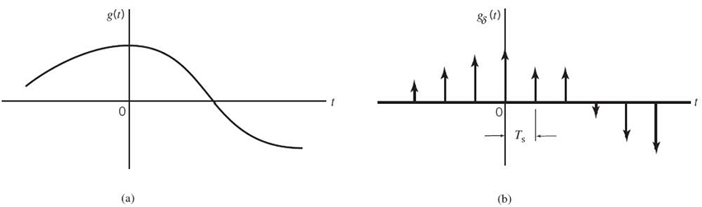
Figure 6.1  The sampling process. (a) Analog signal. (b) Instantaneously sampled version of the analog signal.

Let g_δ(t) denote the signal obtained by individually weighting the elements of a periodic sequence of delta functions spaced T_s seconds apart by the sequence of numbers {g(nT_s)}, as shown by (see Figure 6.1b):

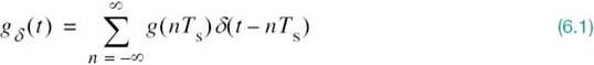
We refer to g_δ(t) as the ideal sampled signal. The term δ(t – nT_s) represents a delta function positioned at time t = nT_s. From the definition of the delta function, we recall from Chapter 2 that such an idealized function has unit area. We may therefore view the multiplying factor g(nT_s) in (6.1) as a “mass” assigned to the delta function δ(t – nT_s). A delta function weighted in this manner is closely approximated by a rectangular pulse of duration Δt and amplitude g(nT_s)/Δt; the smaller we make Δt the better the approximation will be.

Referring to the table of Fourier-transform pairs in Table 2.2, we have

where G(f) is the Fourier transform of the original signal g(t) and f_s is the sampling rate. Equation (6.2) states:

The process of uniformly sampling a continuous-time signal of finite energy results in a periodic spectrum with a frequency equal to the sampling rate.

Another useful expression for the Fourier transform of the ideal sampled signal g_δ(t) may be obtained by taking the Fourier transform of both sides of (6.1) and noting that the Fourier transform of the delta function δ(t – nT_s) is equal to exp(–j2πnfT_s). Letting G_δ(f) denote the Fourier transform of g_δ(t), we may write

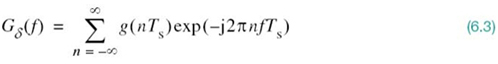
Equation (6.3) describes the discrete-time Fourier transform. It may be viewed as a complex Fourier series representation of the periodic frequency function G_δ(f), with the sequence of samples {g(nT_s)} defining the coefficients of the expansion.

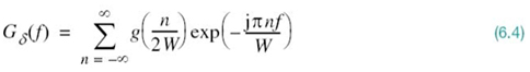
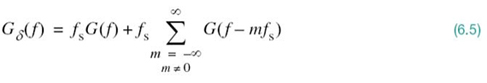
The discussion presented thus far applies to any continuous-time signal g(t) of finite energy and infinite duration. Suppose, however, that the signal g(t) is strictly band limited, with no frequency components higher than W hertz. That is, the Fourier transform G(f) of the signal g(t) has the property that G(f) is zero for | f | ≥ W, as illustrated in Figure 6.2a; the shape of the spectrum shown in this figure is merely intended for the purpose of illustration. Suppose also that we choose the sampling period T_s = 1/2W. Then the corresponding spectrum G_δ(f) of the sampled signal g_δ(t) is as shown in Figure 6.2b. Putting T_s = 1/2W in (6.3) yields

Isolating the term on the right-hand side of (6.2), corresponding to m = 0, we readily see that the Fourier transform of g_δ(t) may also be expressed as

Suppose, now, we impose the following two conditions:

1.  G(f) = 0 for | f | ≥ W.

2.  f_s = 2W.

We may then reduce (6.5) to

Substituting (6.4) into (6.6), we may also write

Equation (6.7) is the desired formula for the frequency-domain description of sampling. This formula reveals that if the sample values g(n/2W) of the signal g(t) are specified for all n, then the Fourier transform G(f) of that signal is uniquely determined. Because g(t) is related to G(f) by the inverse Fourier transform, it follows, therefore, that g(t) is itself uniquely determined by the sample values g(n/2W) for –∞ < n < ∞. In other words, the sequence {g(n/2W)} has all the information contained in the original signal g(t).

Figure 6.2  (a) Spectrum of a strictly band-limited signal g(t). (b) Spectrum of the sampled version of g(t) for a sampling period T_s = 1/2W.

Consider next the problem of reconstructing the signal g(t) from the sequence of sample values {g(n/2W)}. Substituting (6.7) in the formula for the inverse Fourier transform

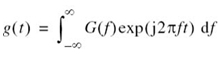
and interchanging the order of summation and integration, which is permissible because both operations are linear, we may go on to write

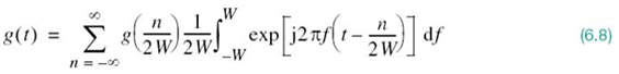
The definite integral in (6.8), including the multiplying factor 1/2W, is readily evaluated in terms of the sinc function, as shown by

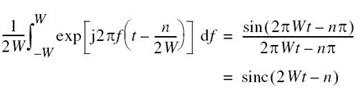
Accordingly, (6.8) reduces to the infinite-series expansion

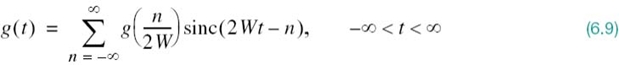
Equation (6.9) is the desired reconstruction formula. This formula provides the basis for reconstructing the original signal g(t) from the sequence of sample values {g(n/2W)}, with the sinc function sinc(2Wt) playing the role of a basis function of the expansion. Each sample, g(n/2W), is multiplied by a delayed version of the basis function, sinc(2Wt – n), and all the resulting individual waveforms in the expansion are added to reconstruct the original signal g(t).

The Sampling Theorem

Equipped with the frequency-domain description of sampling given in (6.7) and the reconstruction formula of (6.9), we may now state the sampling theorem for strictly band-limited signals of finite energy in two equivalent parts:

1.  A band-limited signal of finite energy that has no frequency components higher than W hertz is completely described by specifying the values of the signal instants of time separated by 1/2W seconds.

2.  A band-limited signal of finite energy that has no frequency components higher than W hertz is completely recovered from a knowledge of its samples taken at the rate of 2W samples per second.

Part 1 of the theorem, following from (6.7), is performed in the transmitter. Part 2 of the theorem, following from (6.9), is performed in the receiver. For a signal bandwidth of W hertz, the sampling rate of 2W samples per second, for a signal bandwidth of W hertz, is called the Nyquist rate; its reciprocal 1/2W (measured in seconds) is called the Nyquist interval; see the classic paper (Nyquist, 1928b).

 Aliasing Phenomenon

Derivation of the sampling theorem just described is based on the assumption that the signal g(t) is strictly band limited. In practice, however, a message signal is not strictly band limited, with the result that some degree of undersampling is encountered, as a consequence of which aliasing is produced by the sampling process. Aliasing refers to the phenomenon of a high-frequency component in the spectrum of the signal seemingly taking on the identity of a lower frequency in the spectrum of its sampled version, as illustrated in Figure 6.3. The aliased spectrum, shown by the solid curve in Figure 6.3b, pertains to the undersampled version of the message signal represented by the spectrum of Figure 6.3a.

To combat the effects of aliasing in practice, we may use two corrective measures:

1.  Prior to sampling, a low-pass anti-aliasing filter is used to attenuate those high-frequency components of the signal that are not essential to the information being conveyed by the message signal g(t).

2.  The filtered signal is sampled at a rate slightly higher than the Nyquist rate.

The use of a sampling rate higher than the Nyquist rate also has the beneficial effect of easing the design of the reconstruction filter used to recover the original signal from its sampled version. Consider the example of a message signal that has been anti-alias (low-pass) filtered, resulting in the spectrum shown in Figure 6.4a. The corresponding spectrum of the instantaneously sampled version of the signal is shown in Figure 6.4b, assuming a sampling rate higher than the Nyquist rate. According to Figure 6.4b, we readily see that design of the reconstruction filter may be specified as follows:

• The reconstruction filter is low-pass with a passband extending from –W to W, which is itself determined by the anti-aliasing filter.
• The reconstruction filter has a transition band extending (for positive frequencies) from W to (f_s – W), where f_s is the sampling rate.

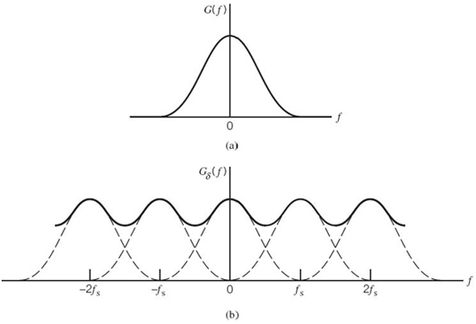
Figure 6.3  (a) Spectrum of a signal. (b) Spectrum of an under-sampled version of the signal exhibiting the aliasing phenomenon.

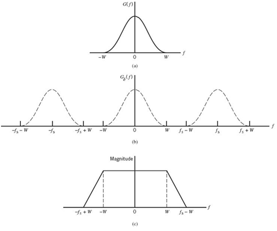
Figure 6.4  (a) Anti-alias filtered spectrum of an information-bearing signal. (b) Spectrum of instantaneously sampled version of the signal, assuming the use of a sampling rate greater than the Nyquist rate. (c) Magnitude response of reconstruction filter.

EXAMPLE 1  Sampling of Voice Signals

As an illustrative example, consider the sampling of voice signals for waveform coding. Typically, the frequency band, extending from 100 Hz to 3.1 kHz, is considered to be adequate for telephonic communication. This limited frequency band is accomplished by passing the voice signal through a low-pass filter with its cutoff frequency set at 3.1 kHz; such a filter may be viewed as an anti-aliasing filter. With such a cutoff frequency, the Nyquist rate is f_s=2 × 3.1 = 6.2 kHz. The standard sampling rate for the waveform coding of voice signals is 8 kHz. Putting these numbers together, design specifications for the reconstruction (low-pass) filter in the receiver are as follows:

Cutoff frequency	3.1 kHz
Transition band	6.2 to 8 kHz
Transition-band width	1.8 kHz.

6.3    Pulse-Amplitude Modulation

Now that we understand the essence of the sampling process, we are ready to formally define PAM, which is the simplest and most basic form of analog pulse modulation. It is formally defined as follows:

PAM is a linear modulation process where the amplitudes of regularly spaced pulses are varied in proportion to the corresponding sample values of a continuous message signal.

The pulses themselves can be of a rectangular form or some other appropriate shape.

The waveform of a PAM signal is illustrated in Figure 6.5. The dashed curve in this figure depicts the waveform of a message signal m(t), and the sequence of amplitude-modulated rectangular pulses shown as solid lines represents the corresponding PAM signal s(t). There are two operations involved in the generation of the PAM signal:

1.  Instantaneous sampling of the message signal m(t) every T_s seconds, where the sampling rate f_s = 1/T_s is chosen in accordance with the sampling theorem.

2.  Lengthening the duration of each sample so obtained to some constant value T.

In digital circuit technology, these two operations are jointly referred to as “sample and hold.” One important reason for intentionally lengthening the duration of each sample is to avoid the use of an excessive channel bandwidth, because bandwidth is inversely proportional to pulse duration. However, care has to be exercised in how long we make the sample duration T, as the following analysis reveals.

Let s(t) denote the sequence of flat-top pulses generated in the manner described in Figure 6.5. We may express the PAM signal as a discrete convolution sum:

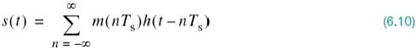
where T_s is the sampling period and m(nT_s) is the sample value of m(t) obtained at time t = nT_s. The h(t) is a Fourier-transformal pulse. With spectral analysis of s(t) in mind, we would like to recast (6.10) in the form of a convolution integral. To this end, we begin by invoking the sifting property of a delta function (discussed in Chapter 2) to express the delayed version of the pulse shape h(t) in (6.10) as

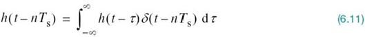
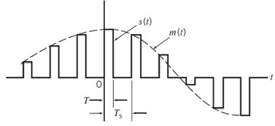
Figure 6.5  Flat-top samples, representing an analog signal.

Hence, substituting (6.11) into (6.10), and interchanging the order of summation and integration, we get

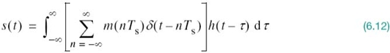
Referring to (6.1), we recognize that the expression inside the brackets in (6.12) is simply the instantaneously sampled version of the message signal m(t), as shown by

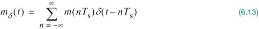
Accordingly, substituting (6.13) into (6.12), we may reformulate the PAM signal s(t) in the desired form

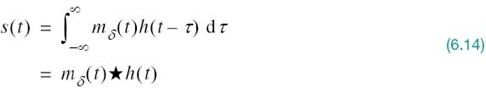
which is the convolution of the two time functions; convolution of the two time functions; m_δ(t)and h(t).

The stage is now set for taking the Fourier transform of both sides of (6.14) and recognizing that the convolution of two time functions is transformed into the multiplication of their respective Fourier transforms; we get the simple result

where S(f) = F[s(t)], M_δ(f) = F[m_δ(t)], and H(f) = F[h(t)]. Adapting (6.2) to the problem at hand, we note that the Fourier transform M_δ(f) is related to the Fourier transform M(f) of the original message signal m(t) as follows:

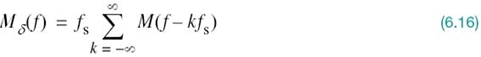
where f_s is the sampling rate. Therefore, the substitution of (6.16) into (6.15) yields the desired formula for the Fourier transform of the PAM signal s(t), as shown by

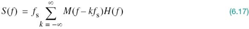
Given this formula, how do we recover the original message signal m(t)? As a first step in this reconstruction, we may pass s(t) through a low-pass filter whose frequency response is defined in Figure 6.4c; here, it is assumed that the message signal is limited to bandwidth W and the sampling rate f_s is larger than the Nyquist rate 2W. Then, from (6.17) we find that the spectrum of the resulting filter output is equal to M(f)H(f). This output is equivalent to passing the original message signal m(t) through another low-pass filter of frequency response H(f).

Equation (6.17) applies to any Fourier-transformable pulse shape h(t).

Consider now the special case of a rectangular pulse of unit amplitude and duration T, as shown in Figure 6.6a; specifically:

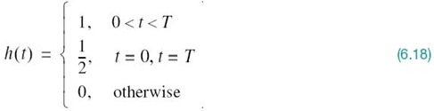
Correspondingly, the Fourier transform of h(t) is given by

which is plotted in Figure 6.6b. We therefore find from (6.17) that by using flat-top samples to generate a PAM signal we have introduced amplitude distortion as well as a delay of T/2. This effect is rather similar to the variation in transmission with frequency that is caused by the finite size of the scanning aperture in television. Accordingly, the distortion caused by the use of PAM to transmit an analog information-bearing signal is referred to as the aperture effect.

To correct for this distortion, we connect an equalizer in cascade with the low-pass reconstruction filter, as shown in Figure 6.7. The equalizer has the effect of decreasing the in-band loss of the reconstruction filter as the frequency increases in such a manner as to

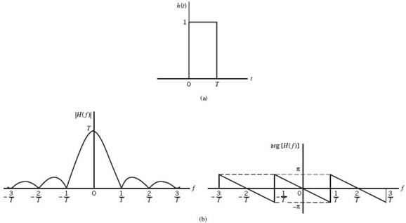
Figure 6.6  (a) Rectangular pulse h(t). (b) Transfer function H(f), made up of the magnitude |H(f)| and phase arg[H(f)].

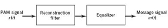
Figure 6.7  System for recovering message signal m(t) from PAM signal s(t).

compensate for the aperture effect. In light of (6.19), the magnitude response of the equalizer should ideally be

The amount of equalization needed in practice is usually small. Indeed, for a duty cycle defined by the ratio T/T_s ≤ 0.1, the amplitude distortion is less than 0.5%. In such a situation, the need for equalization may be omitted altogether.

 Practical Considerations

The transmission of a PAM signal imposes rather stringent requirements on the frequency response of the channel, because of the relatively short duration of the transmitted pulses. One other point that should be noted: relying on amplitude as the parameter subject to modulation, the noise performance of a PAM system can never be better than baseband-signal transmission. Accordingly, in practice, we find that for transmission over a communication channel PAM is used only as the preliminary means of message processing, whereafter the PAM signal is changed to some other more appropriate form of pulse modulation.

With analog-to-digital conversion as the aim, what would be the appropriate form of modulation to build on PAM? Basically, there are three potential candidates, each with its own advantages and disadvantages, as summarized here:

1.  PCM, which, as remarked previously in Section 6.1, is robust but demanding in both transmission bandwidth and computational requirements. Indeed, PCM has established itself as the standard method for the conversion of speech and video signals into digital form.

2.  DPCM, which provides a method for the reduction in transmission bandwidth but at the expense of increased computational complexity.

3.  DM, which is relatively simple to implement but requires a significant increase in transmission bandwidth.

Before we go on, a comment on terminology is in order. The term “modulation” used herein is a misnomer. In reality, PCM, DM, and DPCM are different forms of source coding, with source coding being understood in the sense described in Chapter 5 on information theory. Nevertheless, the terminologies used to describe them have become embedded in the digital communications literature, so much so that we just have to live with them.

Despite their basic differences, PCM, DPCM and DM do share an important feature: the message signal is represented in discrete form in both time and amplitude. PAM takes care of the discrete-time representation. As for the discrete-amplitude representation, we resort to a process known as quantization, which is discussed next.

6.4    Quantization and its Statistical Characterization

Typically, an analog message signal (e.g., voice) has a continuous range of amplitudes and, therefore, its samples have a continuous amplitude range. In other words, within the finite amplitude range of the signal, we find an infinite number of amplitude levels. In actual fact, however, it is not necessary to transmit the exact amplitudes of the samples for the following reason: any human sense (the ear or the eye) as ultimate receiver can detect only finite intensity differences. This means that the message signal may be approximated by a signal constructed of discrete amplitudes selected on a minimum error basis from an available set. The existence of a finite number of discrete amplitude levels is a basic condition of waveform coding exemplified by PCM. Clearly, if we assign the discrete amplitude levels with sufficiently close spacing, then we may make the approximated signal practically indistinguishable from the original message signal. For a formal definition of amplitude quantization, or just quantization for short, we say:

Quantization is the process of transforming the sample amplitude m(nT_s) of a message signal m(t) at time t = nT_s into a discrete amplitude v(nT_s) taken from a finite set of possible amplitudes.

This definition assumes that the quantizer (i.e., the device performing the quantization process) is memoryless and instantaneous, which means that the transformation at time t = nT_s is not affected by earlier or later samples of the message signal m(t). This simple form of scalar quantization, though not optimum, is commonly used in practice.

When dealing with a memoryless quantizer, we may simplify the notation by dropping the time index. Henceforth, the symbol m_k is used in place of m(kT_s), as indicated in the block diagram of a quantizer shown in Figure 6.8a. Then, as shown in Figure 6.8b, the signal amplitude m is specified by the index k if it lies inside the partition cell

where

and L is the total number of amplitude levels used in the quantizer. The discrete amplitudes m_k, k = 1,2,…,L, at the quantizer input are called decision levels or decision thresholds. At the quantizer output, the index k is transformed into an amplitude v_k that represents all amplitudes of the cell J_k; the discrete amplitudes v_k, k = 1,2,…,L, are called representation levels or reconstruction levels. The spacing between two adjacent representation levels is called a quantum or step-size. Thus, given a quantizer denoted by g(·), the quantized output v equals v_k if the input sample m belongs to the interval J_k. In effect, the mapping (see Figure 6.8a)

defines the quantizer characteristic, described by a staircase function.

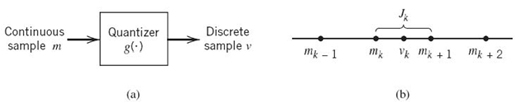
Figure 6.8  Description of a memoryless quantizer.

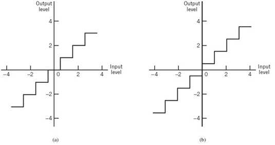
Figure 6.9  Two types of quantization: (a) midtread and (b) midrise.

Quantizers can be of a uniform or nonuniform type. In a uniform quantizer, the representation levels are uniformly spaced; otherwise, the quantizer is nonuniform. In this section, we consider only uniform quantizers; nonuniform quantizers are considered in Section 6.5. The quantizer characteristic can also be of midtread or midrise type. Figure 6.9a shows the input–output characteristic of a uniform quantizer of the midtread type, which is so called because the origin lies in the middle of a tread of the staircaselike graph. Figure 6.9b shows the corresponding input–output characteristic of a uniform quantizer of the midrise type, in which the origin lies in the middle of a rising part of the staircaselike graph. Despite their different appearances, both the midtread and midrise types of uniform quantizers illustrated in Figure 6.9 are symmetric about the origin.

   Quantization Noise

Inevitably, the use of quantization introduces an error defined as the difference between the continuous input sample m and the quantized output sample v. The error is called quantization noise.¹ Figure 6.10 illustrates a typical variation of quantization noise as a function of time, assuming the use of a uniform quantizer of the midtread type.

Let the quantizer input m be the sample value of a zero-mean random variable M. (If the input has a nonzero mean, we can always remove it by subtracting the mean from the input and then adding it back after quantization.) A quantizer, denoted by g(·), maps the input random variable M of continuous amplitude into a discrete random variable V; their respective sample values m and v are related by the nonlinear function g(·) in (6.22). Let the quantization error be denoted by the random variable Q of sample value q. We may thus write

or, correspondingly,

With the input M having zero mean and the quantizer assumed to be symmetric as in Figure 6.9, it follows that the quantizer output V and, therefore, the quantization error Q will also have zero mean. Thus, for a partial statistical characterization of the quantizer in terms of output signal-to-(quantization) noise ratio, we need only find the mean-square value of the quantization error Q.

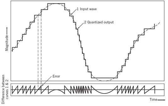
Figure 6.10  Illustration of the quantization process.

Consider, then, an input m of continuous amplitude, which, symmetrically, occupies the range [–m_max, m_max]. Assuming a uniform quantizer of the midrise type illustrated in Figure 6.9b, we find that the step size of the quantizer is given by

where L is the total number of representation levels. For a uniform quantizer, the quantization error Q will have its sample values bounded by –Δ/2 ≤ q ≤ Δ/2. If the step size Δ is sufficiently small (i.e., the number of representation levels L is sufficiently large), it is reasonable to assume that the quantization error Q is a uniformly distributed random variable and the interfering effect of the quantization error on the quantizer input is similar to that of thermal noise, hence the reference to quantization error as quantization noise. We may thus express the probability density function of the quantization noise as

For this to be true, however, we must ensure that the incoming continuous sample does not overload the quantizer. Then, with the mean of the quantization noise being zero, its variance is the same as the mean-square value; that is,

Substituting (6.26) into (6.27), we get

Typically, the L-ary number k, denoting the kth representation level of the quantizer, is transmitted to the receiver in binary form. Let R denote the number of bits per sample used in the construction of the binary code. We may then write

or, equivalently,

Hence, substituting (6.29) into (6.25), we get the step size

Thus, the use of (6.31) in (6.28) yields

Let P denote the average power of the original message signal m(t). We may then express the output signal-to-noise ratio of a uniform quantizer as

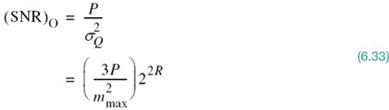
Equation (6.33) shows that the output signal-to-noise ratio of a uniform quantizer (SNR)_O increases exponentially with increasing number of bits per sample R, which is intuitively satisfying.

EXAMPLE 2  Sinusoidal Modulating Signal

Consider the special case of a full-load sinusoidal modulating signal of amplitude A_m, which utilizes all the representation levels provided. The average signal power is (assuming a load of 1 Ω)

The total range of the quantizer input is 2A_m, because the modulating signal swings between –A_m and A_m. We may, therefore, set m_max = A_m, in which case the use of (6.32) yields the average power (variance) of the quantization noise as

Thus, the output signal-to-noise of a uniform quantizer, for a full-load test tone, is

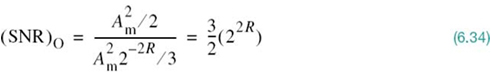
Expressing the signal-to-noise (SNR) in decibels, we get

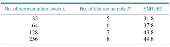
The corresponding values of signal-to-noise ratio for various values of L and R, are given in Table 6.1. For sinusoidal modulation, this table provides a basis for making a quick estimate of the number of bits per sample required for a desired output signal-to-noise ratio.

Table 6.1  Signal-to-(quantization) noise ratio for varying number of representation levels for sinusoidal modulation

 Conditions of Optimality of Scalar Quantizers

In designing a scalar quantizer, the challenge is how to select the representation levels and surrounding partition cells so as to minimize the average quantization power for a fixed number of representation levels.

To state the problem in mathematical terms: consider a message signal m(t) drawn from a stationary process and whose dynamic range, denoted by –A ≤ m ≤ A, is partitioned into a set of L cells, as depicted in Figure 6.11. The boundaries of the partition cells are defined by a set of real numbers m₁, m₂,…,m_{L – 1} that satisfy the following three conditions:

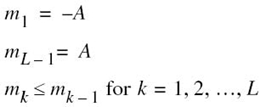
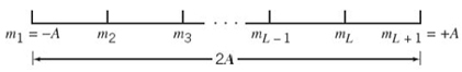
Figure 6.11  Illustrating the partitioning of the dynamic range –A ≤ m ≤ A of a message signal m(t) into a set of L cells.

The kth partition cell is defined by (6.20), reproduced here for convenience:

Let the representation levels (i.e., quantization values) be denoted by v_k, k = 1,2,…,L. Then, assuming that d(m, v_k) denotes a distortion measure for using v_k to represent all those values of the input m that lie inside the partition cell J_k, the goal is to find the two sets and that minimize the average distortion

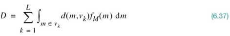
where f_M(m) is the probability density function of the random variable M with sample value m.

A commonly used distortion measure is defined by

in which case we speak of the mean-square distortion. In any event, the optimization problem stated herein is nonlinear, defying an explicit, closed-form solution. To get around this difficulty, we resort to an algorithmic approach for solving the problem in an iterative manner.

Structurally speaking, the quantizer consists of two components with interrelated design parameters:

• An encoder characterized by the set of partition cells ; this is located in the transmitter.
• A decoder characterized by the set of representation levels ; this is located in the receiver.

Accordingly, we may identify two critically important conditions that provide the mathematical basis for all algorithmic solutions to the optimum quantization problem. One condition assumes that we are given a decoder and the problem is to find the optimum encoder in the transmitter. The other condition assumes that we are given an encoder and the problem is to find the optimum decoder in the receiver. Henceforth, these two conditions are referred to as condition I and II, respectively.

Condition I:   Optimality of the Encoder for a Given Decoder

The availability of a decoder means that we have a certain codebook in mind. Let the codebook be defined by

Given the codebook , the problem is to find the set of partition cells that minimizes the mean-square distortion D. That is, we wish to find the encoder defined by the nonlinear mapping

such that we have

For the lower bound specified in (6.41) to be attained, we require that the nonlinear mapping of (6.40) be satisfied only if the condition

The necessary condition described in (6.42) for optimality of the encoder for a specified codebook is recognized as the nearest-neighbor condition. In words, the nearest neighbor condition requires that the partition cell J_k should embody all those values of the input m that are closer to v_k than any other element of the codebook . This optimality condition is indeed intuitively satisfying.

Condition II:   Optimality of the Decoder for a Given Encoder

Consider next the reverse situation to that described under condition I, which may be stated as follows: optimize the codebook for the decoder, given that the set of partition cells characterizing the encoder is fixed. The criterion for optimization is the average (mean-square) distortion:

The probability density function f_M(m) is clearly independent of the codebook . Hence, differentiating D with respect to the representation level v_k, we readily obtain

Setting ∂D/∂v_k equal to zero and then solving for v_k, we obtain the optimum value

The denominator in (6.45) is just the probability p_k that the random variable M with sample value m lies in the partition cell J_k, as shown by

Accordingly, we may interpret the optimality condition of (6.45) as choosing the representation level v_k to equal the conditional mean of the random variable M, given that M lies in the partition cell J_k. We can thus formally state that the condition for optimality of the decoder for a given encoder as follows:

where is the expectation operator. (Equation 6.47) is also intuitively satisfying.

Note that the nearest neighbor condition (I) for optimality of the encoder for a given decoder was proved for a generic average distortion. However, the conditional mean requirement (condition II) for optimality of the decoder for a given encoder was proved for the special case of a mean-square distortion. In any event, these two conditions are necessary for optimality of a scalar quantizer. Basically, the algorithm for designing the quantizer consists of alternately optimizing the encoder in accordance with condition I, then optimizing the decoder in accordance with condition II, and continuing in this manner until the average distortion D reaches a minimum. The optimum quantizer designed in this manner is called the Lloyd–Max quantizer.²

6.5     Pulse-Code Modulation

With the material on sampling, PAM, and quantization presented in the preceding sections, the stage is set for describing PCM, for which we offer the following definition:

PCM is a discrete-time, discrete-amplitude waveform-coding process, by means of which an analog signal is directly represented by a sequence of coded pulses.

Specifically, the transmitter consists of two components: a pulse-amplitude modulator followed by an analog-to-digital (A/D) converter. The latter component itself embodies a quantizer followed by an encoder. The receiver performs the inverse of these two operations: digital-to-analog (D/A) conversion followed by pulse-amplitude demodulation. The communication channel is responsible for transporting the encoded pulses from the transmitter to the receiver.

Figure 6.12, a block diagram of the PCM, shows the transmitter, the transmission path from the transmitter output to the receiver input, and the receiver.

It is important to realize, however, that once distortion in the form of quantization noise is introduced into the encoded pulses, there is absolutely nothing that can be done at the receiver to compensate for that distortion. The only design precaution that can be taken is to choose a number of representation levels in the receiver that is large enough to ensure that the quantization noise is imperceptible for human use at the receiver output.

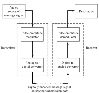
Figure 6.12  Block diagram of PCM system.

 Sampling in the Transmitter

The incoming message signal is sampled with a train of rectangular pulses short enough to closely approximate the instantaneous sampling process. To ensure perfect reconstruction of the message signal at the receiver, the sampling rate must be greater than twice the highest frequency component W of the message signal in accordance with the sampling theorem. In practice, a low-pass anti-aliasing filter is used at the front end of the pulse-amplitude modulator to exclude frequencies greater than W before sampling and which are of negligible practical importance. Thus, the application of sampling permits the reduction of the continuously varying message signal to a limited number of discrete values per second.

 Quantization in the Transmitter

The PAM representation of the message signal is then quantized in the analog-to-digital converter, thereby providing a new representation of the signal that is discrete in both time and amplitude. The quantization process may follow a uniform law as described in Section 6.4. In telephonic communication, however, it is preferable to use a variable separation between the representation levels for efficient utilization of the communication channel. Consider, for example, the quantization of voice signals. Typically, we find that the range of voltages covered by voice signals, from the peaks of loud talk to the weak passages of weak talk, is on the order of 1000 to 1. By using a nonuniform quantizer with the feature that the step size increases as the separation from the origin of the input–output amplitude characteristic of the quantizer is increased, the large end-steps of the quantizer can take care of possible excursions of the voice signal into the large amplitude ranges that occur relatively infrequently. In other words, the weak passages needing more protection are favored at the expense of the loud passages. In this way, a nearly uniform percentage precision is achieved throughout the greater part of the amplitude range of the input signal. The end result is that fewer steps are needed than would be the case if a uniform quantizer were used; hence the improvement in channel utilization.

Assuming memoryless quantization, the use of a nonuniform quantizer is equivalent to passing the message signal through a compressor and then applying the compressed signal to a uniform quantizer, as illustrated in Figure 6.13a. A particular form of compression law that is used in practice is the so-called μ-law,³ which is defined by

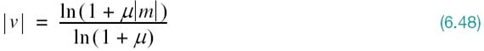
where ln, i.e., log_e, denotes the natural logarithm, m and v are the input and output voltages of the compressor, and μ is a positive constant. It is assumed that m and, therefore, v are scaled so that they both lie inside the interval [–1, 1]. The μ-law is plotted for three different values of μ in Figure 6.14a. The case of uniform quantization corresponds to μ = 0. For a given value of μ, the reciprocal slope of the compression curve that defines the quantum steps is given by the derivative of the absolute value |m| with respect to the corresponding absolute value |v|; that is,

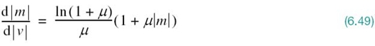
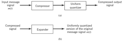
Figure 6.13  (a) Nonuniform quantization of the message signal in the transmitter. (b) Uniform quantization of the original message signal in the receiver.

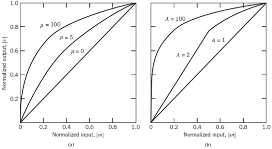
Figure 6.14  Compression laws: (a) μ-law; (b) A-law.

From (6.49) it is apparent that the μ-law is neither strictly linear nor strictly logarithmic. Rather, it is approximately linear at low input levels corresponding to μ|m| ≪ 1 and approximately logarithmic at high input levels corresponding to μ|m| ≫ 1.

Another compression law that is used in practice is the so-called A-law, defined by

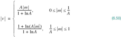
where A is another positive constant. Equation (6.50) is plotted in Figure 6.14b for varying A. The case of uniform quantization corresponds to A = 1. The reciprocal slope of this second compression curve is given by the derivative of |m| with respect to |v|, as shown by

To restore the signal samples to their correct relative level, we must, of course, use a device in the receiver with a characteristic complementary to the compressor. Such a device is called an expander. Ideally, the compression and expansion laws are exactly the inverse of each other. With this provision in place, we find that, except for the effect of quantization, the expander output is equal to the compressor input. The cascade combination of a compressor and an expander, depicted in Figure 6.13, is called a compander.

For both the μ-law and A-law, the dynamic range capability of the compander improves with increasing μ and A, respectively. The SNR for low-level signals increases at the expense of the SNR for high-level signals. To accommodate these two conflicting requirements (i.e., a reasonable SNR for both low- and high-level signals), a compromise is usually made in choosing the value of parameter μ for the μ-law and parameter A for the A-law. The typical values used in practice are μ = 255 for the μ–law and A = 87.6 for the A-law.⁴

 Encoding in the Transmitter

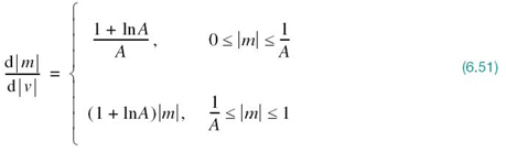
Through the combined use of sampling and quantization, the specification of an analog message signal becomes limited to a discrete set of values, but not in the form best suited to transmission over a telephone line or radio link. To exploit the advantages of sampling and quantizing for the purpose of making the transmitted signal more robust to noise, interference, and other channel impairments, we require the use of an encoding process to translate the discrete set of sample values to a more appropriate form of signal. Any plan for representing each of this discrete set of values as a particular arrangement of discrete events constitutes a code. Table 6.2 describes the one-to-one correspondence between representation levels and codewords for a binary number system for R = 4 bits per sample. Following the terminology of Chapter 5, the two symbols of a binary code are customarily denoted as 0 and 1. In practice, the binary code is the preferred choice for encoding for the following reason:

The maximum advantage over the effects of noise encountered in a communication system is obtained by using a binary code because a binary symbol withstands a relatively high level of noise and, furthermore, it is easy to regenerate.

The last signal-processing operation in the transmitter is that of line coding, the purpose of which is to represent each binary codeword by a sequence of pulses; for example, symbol 1 is represented by the presence of a pulse and symbol 0 is represented by absence of the pulse. Line codes are discussed in Section 6.10. Suppose that, in a binary code, each codeword consists of R bits. Then, using such a code, we may represent a total of 2^R distinct numbers. For example, a sample quantized into one of 256 levels may be represented by an 8-bit codeword.

 Inverse Operations in the PCM Receiver

The first operation in the receiver of a PCM system is to regenerate (i.e., reshape and clean up) the received pulses. These clean pulses are then regrouped into codewords and decoded (i.e., mapped back) into a quantized pulse-amplitude modulated signal. The decoding process involves generating a pulse the amplitude of which is the linear sum of all the pulses in the codeword. Each pulse is weighted by its place value (2⁰, 2¹, 2²,…, 2^{R – 1}) in the code, where R is the number of bits per sample. Note, however, that whereas the analog-to-digital converter in the transmitter involves both quantization and encoding, the digital-to-analog converter in the receiver involves decoding only, as illustrated in Figure 6.12.

Table 6.2  Binary number system for T = 4 bits/sample

The final operation in the receiver is that of signal reconstruction. Specifically, an estimate of the original message signal is produced by passing the decoder output through a low-pass reconstruction filter whose cutoff frequency is equal to the message bandwidth W. Assuming that the transmission link (connecting the receiver to the transmitter) is error free, the reconstructed message signal includes no noise with the exception of the initial distortion introduced by the quantization process.

 PCM Regeneration along the Transmission Path

The most important feature of a PCM systems is its ability to control the effects of distortion and noise produced by transmitting a PCM signal through the channel, connecting the receiver to the transmitter. This capability is accomplished by reconstructing the PCM signal through a chain of regenerative repeaters, located at sufficiently close spacing along the transmission path.

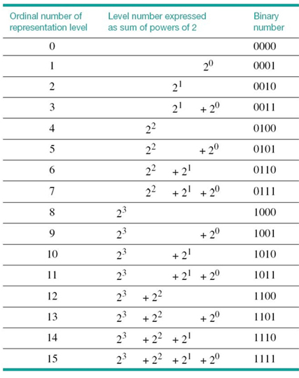
Figure 6.15  Block diagram of regenerative repeater.

As illustrated in Figure 6.15, three basic functions are performed in a regenerative repeater: equalization, timing, and decision making. The equalizer shapes the received pulses so as to compensate for the effects of amplitude and phase distortions produced by the non-ideal transmission characteristics of the channel. The timing circuitry provides a periodic pulse train, derived from the received pulses, for sampling the equalized pulses at the instants of time where the SNR ratio is a maximum. Each sample so extracted is compared with a predetermined threshold in the decision-making device. In each bit interval, a decision is then made on whether the received symbol is 1 or 0 by observing whether the threshold is exceeded or not. If the threshold is exceeded, a clean new pulse representing symbol 1 is transmitted to the next repeater; otherwise, another clean new pulse representing symbol 0 is transmitted. In this way, it is possible for the accumulation of distortion and noise in a repeater span to be almost completely removed, provided that the disturbance is not too large to cause an error in the decision-making process. Ideally, except for delay, the regenerated signal is exactly the same as the signal originally transmitted. In practice, however, the regenerated signal departs from the original signal for two main reasons:

1.  The unavoidable presence of channel noise and interference causes the repeater to make wrong decisions occasionally, thereby introducing bit errors into the regenerated signal.

2.  If the spacing between received pulses deviates from its assigned value, a jitter is introduced into the regenerated pulse position, thereby causing distortion.

The important point to take from this subsection on PCM is the fact that regeneration along the transmission path is provided across the spacing between individual regenerative repeaters (including the last stage of regeneration at the receiver input) provided that the spacing is short enough. If the transmitted SNR ratio is high enough, then the regenerated PCM data stream is the same as the transmitted PCM data stream, except for a practically negligibly small bit error rate (BER). In other words, under these operating conditions, performance degradation in the PCM system is essentially confined to quantization noise in the transmitter.

6.6   Noise Considerations in PCM Systems

The performance of a PCM system is influenced by two major sources of noise:

1.  Channel noise, which is introduced anywhere between the transmitter output and the receiver input; channel noise is always present, once the equipment is switched on.

2.  Quantization noise, which is introduced in the transmitter and is carried all the way along to the receiver output; unlike channel noise, quantization noise is signal dependent, in the sense that it disappears when the message signal is switched off.

Naturally, these two sources of noise appear simultaneously once the PCM system is in operation. However, the traditional practice is to consider them separately, so that we may develop insight into their individual effects on the system performance.

The main effect of channel noise is to introduce bit errors into the received signal. In the case of a binary PCM system, the presence of a bit error causes symbol 1 to be mistaken for symbol 0, or vice versa. Clearly, the more frequently bit errors occur, the more dissimilar the receiver output becomes compared with the original message signal. The fidelity of information transmission by PCM in the presence of channel noise may be measured in terms of the average probability of symbol error, which is defined as the probability that the reconstructed symbol at the receiver output differs from the transmitted binary symbol on the average. The average probability of symbol error, also referred to as the BER, assumes that all the bits in the original binary wave are of equal importance. When, however, there is more interest in restructuring the analog waveform of the original message signal, different symbol errors may be weighted differently; for example, an error in the most significant bit in a codeword (representing a quantized sample of the message signal) is more harmful than an error in the least significant bit.

To optimize system performance in the presence of channel noise, we need to minimize the average probability of symbol error. For this evaluation, it is customary to model the channel noise as an ideal additive white Gaussian noise (AWGN) channel. The effect of channel noise can be made practically negligible by using an adequate signal energy-to-noise density ratio through the provision of short-enough spacing between the regenerative repeaters in the PCM system. In such a situation, the performance of the PCM system is essentially limited by quantization noise acting alone.

From the discussion of quantization noise presented in Section 6.4, we recognize that quantization noise is essentially under the designer’s control. It can be made negligibly small through the use of an adequate number of representation levels in the quantizer and the selection of a companding strategy matched to the characteristics of the type of message signal being transmitted. We thus find that the use of PCM offers the possibility of building a communication system that is rugged with respect to channel noise on a scale that is beyond the capability of any analog communication system; hence its use as a standard against which other waveform coders (e.g., DPCM and DM) are compared.

 Error Threshold

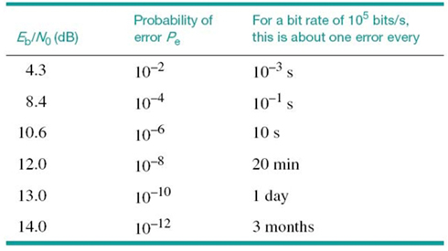
The underlying theory of BER calculation in a PCM system is deferred to Chapter 8. For the present, it suffices to say that the average probability of symbol error in a binary encoded PCM receiver due to AWGN depends solely on E_b/N₀, which is defined as the ratio of the transmitted signal energy per bit E_b, to the noise spectral density N₀. Note that the ratio E_b/N₀ is dimensionless even though the quantities E_b and N₀ have different physical meaning. In Table 6.3, we present a summary of this dependence for the case of a binary PCM system, in which symbols 1 and 0 are represented by rectangular pulses of equal but opposite amplitudes. The results presented in the last column of the table assume a bit rate of 10⁵ bits/s.

From Table 6.3 it is clear that there is an error threshold (at about 11 dB). For E_b/N₀ below the error threshold the receiver performance involves significant numbers of errors, and above it the effect of channel noise is practically negligible. In other words, provided that the ratio E_b/N₀ exceeds the error threshold, channel noise has virtually no effect on the receiver performance, which is precisely the goal of PCM. When, however, E_b/N₀ drops below the error threshold, there is a sharp increase in the rate at which errors occur in the receiver. Because decision errors result in the construction of incorrect codewords, we find that when the errors are frequent, the reconstructed message at the receiver output bears little resemblance to the original message signal.

Table 6.3  Influence of E_b/N₀ on the probability of error

An important characteristic of a PCM system is its ruggedness to interference, caused by impulsive noise or cross-channel interference. The combined presence of channel noise and interference causes the error threshold necessary for satisfactory operation of the PCM system to increase. If, however, an adequate margin over the error threshold is provided in the first place, the system can withstand the presence of relatively large amounts of interference. In other words, a PCM system is robust with respect to channel noise and interference, providing further confirmation to the point made in the previous section that performance degradation in PCM is essentially confined to quantization noise in the transmitter.

 PCM Noise Performance Viewed in Light of the Information Capacity Law

Consider now a PCM system that is known to operate above the error threshold, in which case we would be justified to ignore the effect of channel noise. In other words, the noise performance of the PCM system is essentially determined by quantization noise acting alone. Given such a scenario, how does the PCM system fare compared with the information capacity law, derived in Chapter 5?

To address this question of practical importance, suppose that the system uses a codeword consisting of n symbols with each symbol representing one of M possible discrete amplitude levels; hence the reference to the system as an “M-ary” PCM system. For this system to operate above the error threshold, there must be provision for a large enough noise margin.

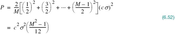
For the PCM system to operate above the error threshold as proposed, the requirement for a noise margin that is sufficiently large to maintain a negligible error rate due to channel noise. This, in turn, means there must be a certain separation between the M discrete amplitude levels. Call this separation cσ, where c is a constant and σ² = N₀B is the noise variance measured in a channel bandwidth B. The number of amplitude levels M is usually an integer power of 2. The average transmitted power will be least if the amplitude range is symmetrical about zero. Then, the discrete amplitude levels, normalized with respect to the separation cσ, will have the values ±1/2, ±3/2,…, ±(M – 1)/2. We assume that these M different amplitude levels are equally likely. Accordingly, we find that the average transmitted power is given by

Suppose that the M-ary PCM system described herein is used to transmit a message signal with its highest frequency component equal to W hertz. The signal is sampled at the Nyquist rate of 2W samples per second. We assume that the system uses a quantizer of the midrise type, with L equally likely representation levels. Hence, the probability of occurrence of any one of the L representation levels is 1/L. Correspondingly, the amount of information carried by a single sample of the signal is log₂ L bits. With a maximum sampling rate of 2W samples per second, the maximum rate of information transmission of the PCM system measured in bits per second is given by

Since the PCM system uses a codeword consisting of n code elements with each one having M possible discrete amplitude values, we have Mⁿ different possible codewords. For a unique encoding process, therefore, we require

Clearly, the rate of information transmission in the system is unaffected by the use of an encoding process. We may, therefore, eliminate L between (6.53) and (6.54) to obtain

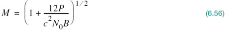
Equation (6.52) defines the average transmitted power required to maintain an M-ary PCM system operating above the error threshold. Hence, solving this equation for the number ofdiscrete amplitude levels, we may express the numberM in terms of the average transmitted power P and channel noise variance σ² = N₀B as follows:

Therefore, substituting (6.56) into (6.55), we obtain

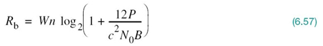
The channel bandwidth B required to transmit a rectangular pulse of duration 1/(2nW), representing a symbol in the codeword, is given by

where κ is a constant with a value lying between 1 and 2. Using the minimum possible value κ = 1, we find that the channel bandwidth B = nW. We may thus rewrite (6.57) as

which defines the upper bound on the information capacity realizable by an M-ary PCM system.

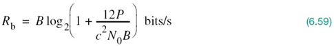
From Chapter 5 we recall that, in accordance with Shannon’s information capacity law, the ideal transmission system is described by the formula

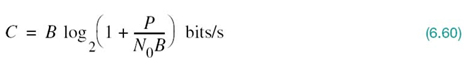
The most interesting point derived from the comparison of (6.59) with (6.60) is the fact that (6.59) is of the right mathematical form in an information-theoretic context. To be more specific, we make the following statement:

Power and bandwidth in a PCM system are exchanged on a logarithmic basis, and the information capacity of the system is proportional to the channel bandwidth B.

As a corollary, we may go on to state:

When the SNR ratio is high, the bandwidth-noise trade-off follows an exponential law in PCM.

From the study of noise in analog modulation systems,⁵ it is known that the use of frequency modulation provides the best improvement in SNR ratio. To be specific, when the carrier-to-noise ratio is high enough, the bandwidth-noise trade-off follows a square law in frequency modulation (FM). Accordingly, in comparing the noise performance of FM with that of PCM we make the concluding statement:

PCM is more efficient than FM in trading off an increase in bandwidth for improved noise performance.

Indeed, this statement is further testimony for the PCM being viewed as a standard for waveform coding.

6.7  Prediction-Error Filtering for Redundancy Reduction

When a voice or video signal is sampled at a rate slightly higher than the Nyquist rate, as usually done in PCM, the resulting sampled signal is found to exhibit a high degree of correlation between adjacent samples. The meaning of this high correlation is that, in an average sense, the signal does not change rapidly from one sample to the next. As a result, the difference between adjacent samples has a variance that is smaller than the variance of the original signal. When these highly correlated samples are encoded, as in the standard PCM system, the resulting encoded signal contains redundant information. This kind of signal structure means that symbols that are not absolutely essential to the transmission of information are generated as a result of the conventional encoding process described in Section 6.5. By reducing this redundancy before encoding, we obtain a more efficient coded signal, which is the basic idea behind DPCM. Discussion of this latter form of waveform coding is deferred to the next section. In this section we discuss prediction-error filtering, which provides a method for reduction and, therefore, improved waveform coding.

 Theoretical Considerations

To elaborate, consider the block diagram of Figure 6.16a, which includes:

• a direct forward path from the input to the output;
• a predictor in the forward direction as well; and
• a comparator for computing the difference between the input signal and the predictor output.

The difference signal, so computed, is called the prediction error. Correspondingly, a filter that operates on the message signal to produce the prediction error, illustrated in Figure 6.16a, is called a prediction-error filter.

To simplify the presentation, let

denote a sample of the message signal m(t) taken at time t = nT_s. Then, with m̂_n denoting the corresponding predictor output, the prediction error is defined by

where e_n is the amount by which the predictor fails to predict the input sample m_n exactly. In any case, the objective is to design the predictor so as to minimize the variance of the prediction error e_n. In so doing, we effectively end up using a smaller number of bits to represent e_n than the original message sample m_n; hence, the need for a smaller transmission bandwidth.

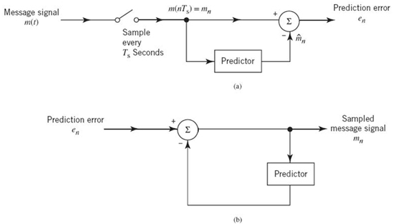
Figure 6.16  Block diagram of (a) prediction-error filter and (b) its inverse.

The prediction-error filter operates on the message signal on a sample-by-sample basis to produce the prediction error. With such an operation performed in the transmitter, how do we recover the original message signal from the prediction error at the receiver? To address this fundamental question in a simple-minded and yet practical way, we invoke the use of linerarity. Let the operator L denote the action of the predictor, as shown by

Accordingly, we may rewrite (6.62) in operator form as follows:

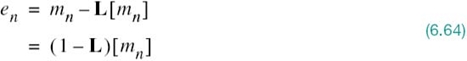
Under the assumption of linearity, we may invert (6.64) to recover the message sample from the prediction error, as shown by

Equation (6.65) is immediately recognized as the equation of a feedback system, as illustrated in Figure 6.16b. Most importantly, in functional terms, this feedback system may be viewed as the inverse of prediction-error filtering.

 Discrete-Time Structure for Prediction

To simplify the design of the linear predictor in Figure 6.16, we propose to use a discrete-time structure in the form of a finite-duration impulse response (FIR) filter, which is well known in the digital signal-processing literature. The FIR filter was briefly discussed in Chapter 2.

Figure 6.17 depicts an FIR filter, consisting of two functional components:

• a set of p unit-delay elements, each of which is represented by z^–1; and
• a corresponding set of adders used to sum the scaled versions of the delayed inputs,

The overall linearly predicted output is thus defined by the convolution sum

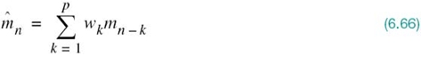
where p is called the prediction order. Minimization of the prediction-error variance is achieved by a proper choice of the FIR filter-coefficients as described next.

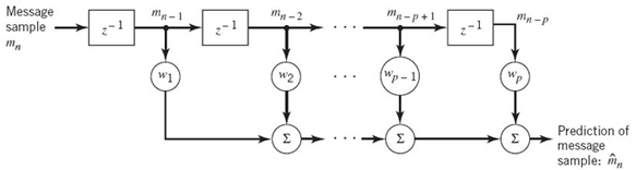
Figure 6.17  Block diagram of an FIR filter of order p.

First, however, we make the following assumption:

The message signal m(t) is drawn from a stationary stochastic processor M(t) with zero mean.

This assumption may be satisfied by processing the message signal on a block-by-block basis, with each block being just long enough to satisfy the assumption in a pseudo-stationary manner. For example, a block duration of 40 ms is considered to be adequate for voice signals.

With the random variable M_n assumed to have zero mean, it follows that the variance of the prediction error e_n is the same as its mean-square value. We may thus define

as the index of performance. Substituting (6.65) and (6.66) into (6.67) and then expanding terms, the index of performance is expressed as follows:

Moreover, under the above assumption of pseudo-stationarity, we may go on to introduce the following second-order statistical parameters for m_n treated as a sample of the stochastic process M(t) at t = nT_s:

1.  Variance

2.  Autocorrelation function

Note that to simplify the notation in (6.67) to (6.70), we have applied the expectation operator to samples rather than the corresponding random variables.

In any event, using (6.69) and (6.70), we may reformulate the index of performance of (6.68) in the new form involving statistical parameters:

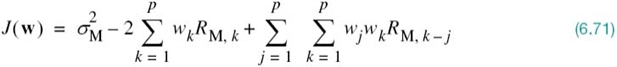
Differentiating this index of performance with respect to the filter coefficients, setting the resulting expression equal to zero, and then rearranging terms, we obtain the following system of simultaneous equations:

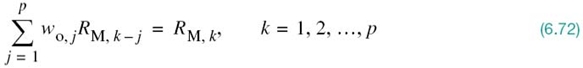
where w_o, _j is the optimal value of the jth filter coefficient w_j. This optimal set of equations is the discrete-time version of the celebrated Wiener–Hopf equations for linear prediction.

With compactness of mathematical exposition in mind, we find it convenient to formulate the Wiener–Hopf equations in matrix form, as shown by

where

is the p-by-1 optimum coefficient vector of the FIR predictor,

is the p-by-1 autocorrelation vector of the original message signal, excluding the mean-square value represented by R_{M, 0}, and

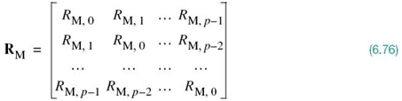
is the p-by-y correlation matrix of the original message signal, including R_{M, 0}.⁶

Careful examination of (6.76) reveals the Toeplitz property of the autocorrelation matrix R_M, which embodies two distinctive characteristics:

1.  All the elements on the main diagonal of the matrix R_M are equal to the mean-square value or, equivalently under the zero-mean assumption, the variance of the message sample m_n, as shown by

2.  The matrix is symmetric about the main diagonal.

This Toeplitz property is a direct consequence of the assumption that message signal m(t) is the sample function of a stationary stochastic process. From a practical perspective, the Toeplitz property of the autocorrelation matrix R_M is important in that all of its elements are uniquely defined by the autocorrelation sequence . Moreover, from the defining equation (6.75), it is clear that the autocorrelation vector r_M is uniquely defined by the autocorrelation sequence . We may therefore make the following statement:

The p filter coefficients of the optimized linear predictor, configured in the form of an FIR filter, are uniquely defined by the variance and the autocorrelation sequence , which pertain to the message signal m(t) drawn from a weakly stationary process.

Typically, we have

Under this condition, we find that the autocorrelation matrix R_M is also invertible; that is, the inverse matrix exists. We may therefore solve (6.73) for the unknown value of the optimal coefficient vector w_o using the formula⁷

Thus, given the variance and autocorrelation sequence , we may uniquely determine the optimized coefficient vector of the linear predictor, w_o, defining an FIR filter of order p; and with it our design objective is satisfied.

To complete the linear prediction theory presented herein, we need to find the minimum mean-square value of prediction error, resulting from the use of the optimized predictor. We do this by first reformulating (6.71) in the matrix form:

where the superscript T denotes matrix transposition, is the inner product of the p-by-1 vectors w_o and r_M, and the matrix product is a quadratic form. Then, substituting the optimum formula of (6.77) into (6.78), we find that the minimum mean-square value of prediction error is given by

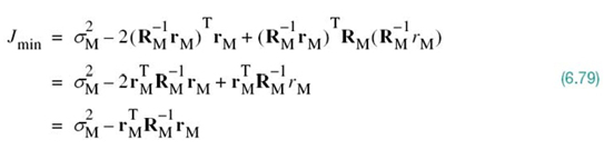
where we have used the property that the autocorrelation matrix of a weakly stationary process is symmetric; that is,

By definition, the quadratic form is always positive. Accordingly, from (6.79) it follows that the minimum value of the mean-square prediction error J_min is always smaller than the variance of the zero-mean message sample m_n that is being predicted. Through the use of linear prediction as described herein, we have thus satisfied the objective:

To design a prediction-error filter the output of which has a smaller variance than the variance of the message sample applied to its input, we need to follow the optimum formula of (6.77).

This statement provides the rationale for going on to describe how the bandwidth requirement of the standard PCM can be reduced through redundancy reduction. However, before proceeding to do so, it is instructive that we consider an adaptive implementation of the linear predictor.

 Linear Adaptive Prediction

The use of (6.77) for calculating the optimum weight vector of a linear predictor requires knowledge of the autocorrelation function R_{m, k} of the message signal sequence where p is the prediction order. What if knowledge of this sequence is not available? In situations of this kind, which occur frequently in practice, we may resort to the use of an adaptive predictor.

The predictor is said to be adaptive in the following sense:

• Computation of the tap weights w_k, k = 1,2,…,p, proceeds in an iterative manner, starting from some arbitrary initial values of the tap weights.
• The algorithm used to adjust the tap weights (from one iteration to the next) is “self-designed, ” operating solely on the basis of available data.

The aim of the algorithm is to find the minimum point of the bowl-shaped error surface that describes the dependence of the cost function J on the tap weights. It is, therefore, intuitively reasonable that successive adjustments to the tap weights of the predictor be made in the direction of the steepest descent of the error surface; that is, in a direction opposite to the gradient vector whose elements are defined by

This is indeed the idea behind the method of deepest descent. Let w_{k, n} denote the value of the kth tap weight at iteration n. Then, the updated value of this weight at iteration n + 1 is defined by

where μ is a step-size parameter that controls the speed of adaptation and the factor 1/2 is included for convenience of presentation. Differentiating the cost function J of (6.68) with respect to w_k, we readily find that

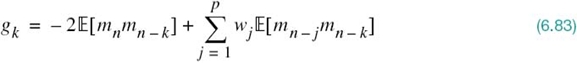
From a practical perspective, the formula for the gradient g_k in (6.83) could do with further simplification that ignores the expectation operator. In effect, instantaneous values are used as estimates of autocorrelation functions. The motivation for this simplification is to permit the adaptive process to proceed forward on a step-by-step basis in a self-organized manner. Clearly, by ignoring the expectation operator in (6.83), the gradient g_k takes on a time-dependent value, denoted by g_{k, n}. We may thus write

where ŵ_{j, n} is an estimate of the filter coefficient w_{j, n} at time n.

The stage is now set for substituting (6.84) into (6.82), where in the latter equation ŵ_{k, n} is substituted for w_{k, n}; this change is made to account for dispensing with the expectation operator:

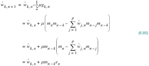
where e_n is the new prediction error defined by

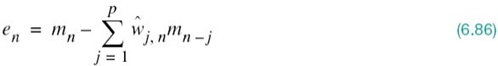
Note that the current value of the message signal, m_n, plays a role as the desired response for predicting the value of m_n given the past values of the message signal: m_{n – 1}, m_{n – 2}, …, m_{n – p}.

In words, we may express the adaptive filtering algorithm of (6.85) as follows:

The algorithm just described is the popular least-mean-square (LMS) algorithm, formulated for the purpose of linear prediction. The reason for popularity of this adaptive filtering algorithm is the simplicity of its implementation. In particular, the computational complexity of the algorithm, measured in terms of the number of additions and multiplications, is linear in the prediction order p. Moreover, the algorithm is not only computationally efficient but it is also effective in performance.

The LMS algorithm is a stochastic adaptive filtering algorithm, stochastic in the sense that, starting from the initial condition defined by , it seeks to find the minimum point of the error surface by following a zig-zag path. However, it never finds this minimum point exactly. Rather, it continues to execute a random motion around the minimum point of the error surface (Haykin, 2013).

6.8    Differential Pulse-Code Modulation

DPCM, the scheme to be considered for channel-bandwidth conservation, exploits the idea of linear prediction theory with a practical difference:

In the transmitter, the linear prediction is performed on a quantized version of the message sample instead of the message sample itself, as illustrated in Figure 6.18.

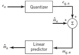
Figure 6.18  Block diagram of a differential quantizer.

The resulting process is referred to as differential quantization. The motivation behind the use of differential quantization follows from two practical considerations:

1.  Waveform encoding in the transmitter requires the use of quantization.

2.  Waveform decoding in the receiver, therefore, has to process a quantized signal.

In order to cater to both requirements in such a way that the same structure is used for predictors in both the transmitter and the receiver, the transmitter has to perform prediction-error filtering on the quantized version of the message signal rather than the signal itself, as shown in Figure 6.19. Then, assuming a noise-free channel, the predictors in the transmitter and receiver operate on exactly the same sequence of quantized message samples.

To demonstrate this highly desirable and distinctive characteristic of differential PCM, we see from Figure 6.19a that

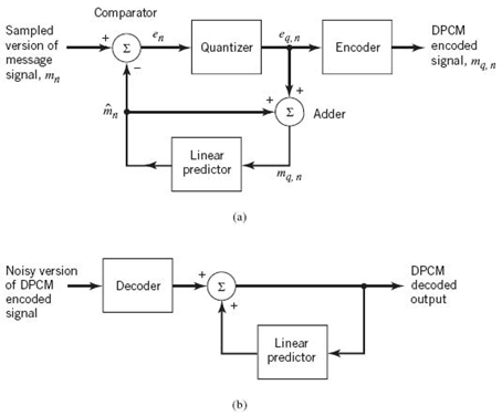
Figure 6.19  DPCM system: (a) transmitter; (b) receiver.

where q_n is the quantization noise produced by the quantizer operating on the prediction error e_n. Moreover, from Figure 6.19a, we readily see that

where m̂_n is the predicted value of the original message sample m_n; thus, (6.88) is in perfect agreement with Figure 6.18. Hence, the use of (6.87) in (6.88) yields

We may now invoke (6.88) of linear prediction theory to rewrite (6.89) in the equivalent form:

which describes a quantized version of the original message sample m_n.

With the differential quantization scheme of Figure 6.19a at hand, we may now expand on the structures of the transmitter and receiver of DPCM.

 DPCM Transmitter

Operation of the DPCM transmitter proceeds as follows:

1.  Given the predicted message sample m̂_n, the comparator at the transmitter input computes the prediction error e_n, which is quantized to produce the quantized version of e_n in accordance with (6.87).

2.  With m̂_n and e_{q, n} at hand, the adder in the transmitter produces the quantized version of the original message sample m_n, namely m_{q, n}, in accordance with (6.88).

3. The required one-step prediction m̂_n is produced by applying the sequence of quantized samples to a linear FIR predictor of order p.

This multistage operation is clearly cyclic, encompassing three steps that are repeated at each time step n. Moreover, at each time step, the encoder operates on the quantized prediction error e_{q, n} to produce the DPCM-encoded version of the original message sample m_n. The DPCM code so produced is a lossy-compressed version of the PCM code;it is “lossy” because of the prediction error.

 DPCM Receiver

The structure of the receiver is much simpler than that of the transmitter, as depicted in Figure 6.19b. Specifically, first, the decoder reconstructs the quantized version of the prediction error, namely e_{q, n}. An estimate of the original message sample m_n is then computed by applying the decoder output to the same predictor used in the transmitter of Figure 6.19a. In the absence of channel noise, the encoded signal at the receiver input is identical to the encoded signal at the transmitter output. Under this ideal condition, we find that the corresponding receiver output is equal to m_{q, n}, which differs from the original signal sample m_n only by the quantization error q_n incurred as a result of quantizing the prediction error e_n.

From the foregoing analysis, we thus observe that, in a noise-free environment, the linear predictors in the transmitter and receiver of DPCM operate on the same sequence of samples, m_{q, n}. It is with this point in mind that a feedback path is appended to the quantizer in the transmitter of Figure 6.19a.

 Processing Gain

The output SNR of the DPCM system, shown in Figure 6.19, is, by definition,

where is the variance of the original signal sample m_n, assumed to be of zero mean, and is the variance of the quantization error q_n, also of zero mean. We may rewrite (6.91) as the product of two factors, as shown by

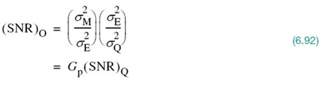
where, in the first line, is the variance of the prediction error e_n. The factor (SNR)_Q introduced in the second line is the signal-to-quantization noise ratio, which is itself defined by

The other factor G_p is the processing gain produced by the differential quantization scheme; it is formally defined by

The quantity G_p, when it is greater than unity, represents a gain in signal-to-noise ratio, which is due to the differential quantization scheme of Figure 6.19. Now, for a given message signal, the variance is fixed, so that G_p is maximized by minimizing the variance of the prediction error e_n. Accordingly, the objective in implementing the DPCM should be to design the prediction filter so as to minimize the prediction-error variance, .

In the case of voice signals, it is found that the optimum signal-to-quantization noise advantage of the DPCM over the standard PCM is in the neighborhood of 4–11dB. Based on experimental studies, it appears that the greatest improvement occurs in going from no prediction to first-order prediction, with some additional gain resulting from increasing the order p of the prediction filter up to 4 or 5, after which little additional gain is obtained. Since 6 dB of quantization noise is equivalent to 1 bit per sample by virtue of the results presented in Table 6.1 for sinusoidal modulation, the advantage of DPCM may also be expressed in terms of bit rate. For a constant signal-to-quantization noise ratio, and assuming a sampling rate of 8 kHz, the use of DPCM may provide a saving of about 8–16 kHz (i.e., 1 to 2 bits per sample) compared with the standard PCM.

6.9    Delta Modulation

In choosing DPCM for waveform coding, we are, in effect, economizing on transmission bandwidth by increasing system complexity, compared with standard PCM. In otherwords, DPCM exploits the complexity–bandwidth tradeoff. However, in practice, the need may arise for reduced system complexity compared with the standard PCM. To achieve this other objective, transmission bandwidth is traded off for reduced system complexity, which is precisely the motivation behind DM. Thus, whereas DPCM exploits the complexity–bandwidth tradeoff, DM exploits the bandwidth–complexity tradeoff. We may, therefore, differentiate between the standard PCM, the DPCM, and the DM along the lines described in Figure 6.20. With the bandwidth–complexity tradeoff being at the heart of DM, the incoming message signal m(t) is oversampled, which requires the use of a sampling rate higher than the Nyquist rate. Accordingly, the correlation between adjacent samples of the message signal is purposely increased so as to permit the use of a simple quantizing strategy for constructing the encoded signal.

 DM Transmitter

In the DM transmitter, system complexity is reduced to the minimum possible by using the combination of two strategies:

1.  Single-bit quantizer, which is the simplest quantizing strategy; as depicted in Figure 6.21, the quantizer acts as a hard limiter with only two decision levels, namely, ±Δ.

2.  Single unit-delay element, which is the most primitive form of a predictor; in other words, the only component retained in the FIR predictor of Figure 6.17 is the front-end block labeled z^–1, which acts as an accumulator.

Thus, replacing the multilevel quantizer and the FIR predictor in the DPCM transmitter of Figure 6.19a in the manner described under points 1 and 2, respectively, we obtain the block diagram of Figure 6.21a for the DM transmitter.

From this figure, we may express the equations underlying the operation of the DM transmitter by the following set of equations (6.95)–(6.97):

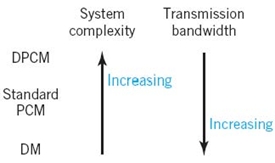
Figure 6.20  Illustrating the tradeoffs between standard PCM, DPCM, and DM.

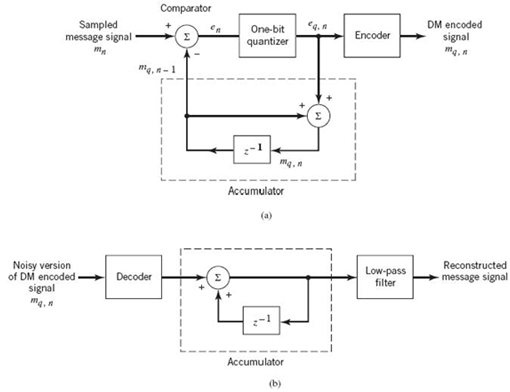
Figure 6.21  DM system: (a) transmitter; (b) receiver.

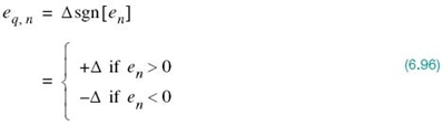
According to (6.95) and (6.96), two possibilities may naturally occur:

1.  The error signal e_n (i.e., the difference between the message sample m_n and its approximation m̂_n) is positive, in which case the approximation m̂_n = m_{q, n – 1} is increased by the amount Δ in this first case, the encoder sends out symbol 1.

2.  The error signal e_n is negative, in which case the approximation m̂_n = m_{q, n – 1} is reduced by the amount Δ in this second case, the encoder sends out symbol 0.

From this description it is apparent that the delta modulator produces a staircase approximation to the message signal, as illustrated in Figure 6.22a. Moreover, the rate of data transmission in DM is equal to the sampling rate f_s = 1/T_s, as illustrated in the binary sequence of Figure 6.22b.

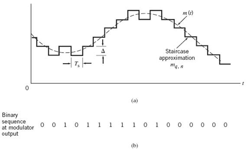
Figure 6.22  Illustration of DM.

 DM Receiver

Following a procedure similar to the way in which we constructed the DM transmitter of Figure 6.21a, we may construct the DM receiver of Figure 6.21b as a special case of the DPCM receiver of Figure 6.19b. Working through the operation of the DM receiver, we find that reconstruction of the staircase approximation to the original message signal is achieved by passing the sequence of positive and negative pulses (representing symbols 1 and 0, respectively) through the block labeled “accumulator.”

Under the assumption that the channel is distortionless, the accumulated output is the desired m_{q, n} given that the decoded channel output is e_{q, n}. The out-of-band quantization noise in the high-frequency staircase waveform in the accumulator output is suppressed by passing it through a low-pass filter with a cutoff frequency equal to the message bandwidth.

 Quantization Errors in DM

DM is subject to two types of quantization error: slope overload distortion and granular noise. We will discuss the case of slope overload distortion first.

Starting with (6.97), we observe that this equation is the digital equivalent of integration, in the sense that it represents the accumulation of positive and negative increments of magnitude Δ. Moreover, denoting the quantization error applied to the message sample m_n by q_n, we may express the quantized message sample as

With this expression for m_{q, n} at hand, we find from (6.98) that the quantizer input is

Thus, except for the delayed quantization error q_n –1, the quantizer input is a first backward difference of the original message sample. This difference may be viewed as a digital approximation to the quantizer input or, equivalently, as the inverse of the digital integration process carried out in the DM transmitter. If, then, we consider the maximum slope of the original message signal m(t), it is clear that in order for the sequence of samples {m_{q, n}} to increase as fast as the sequence of message samples {m_n} in a region of maximum slope of m(t), we require that the condition

be satisfied. Otherwise, we find that the step-size Δ is too small for the staircase approximation m_q(t) to follow a steep segment of the message signal m(t), with the result that m_q(t) falls behind m(t), as illustrated in Figure 6.23. This condition is called slope overload, and the resulting quantization error is called slope-overload distortion (noise). Note that since the maximum slope of the staircase approximation m_q(t) is fixed by the step size Δ, increases and decreases in m_q(t) tend to occur along straight lines. For this reason, a delta modulator using a fixed step size is often referred to as a linear delta modulator.

In contrast to slope-overload distortion, granular noise occurs when the step size Δ is too large relative to the local slope characteristics of the message signal m(t), thereby causing the staircase approximation m_q(t) to hunt around a relatively flat segment of m(t);this phenomenon is also illustrated in the tail end of Figure 6.23. Granular noise is analogous to quantization noise in a PCM system.

 Adaptive DM

From the discussion just presented, it is appropriate that we need to have a large step size to accommodate a wide dynamic range, whereas a small step size is required for the accurate representation of relatively low-level signals. It is clear, therefore, that the choice of the optimum step size that minimizes the mean-square value of the quantization error in a linear delta modulator will be the result of a compromise between slope-overload distortion and granular noise. To satisfy such a requirement, we need to make the delta modulator “adaptive, ” in the sense that the step size is made to vary in accordance with the input signal. The step size is thereby made variable, such that it is enlarged during intervals when the slope-overload distortion is dominant and reduced in value when the granular (quantization) noise is dominant.

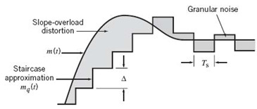
Figure 6.23  Illustration of the two different forms of quantization error in DM.

6.10  Line Codes

In this chapter, we have described three basic waveform-coding schemes: PCM, DPCM, and DM. Naturally, they differ from each other in several ways: transmission–bandwidth requirement, transmitter–receiver structural composition and complexity, and quantization noise. Nevertheless, all three of them have a common need: line codes for electrical representation of the encoded binary streams produced by their individual transmitters, so as to facilitate transmission of the binary streams across the communication channel.

Figure 6.24 displays the waveforms of five important line codes for the example data stream 01101001. Figure 6.25 displays their individual power spectra (for positive frequencies) for randomly generated binary data, assuming that first, symbols 0 and 1 are equiprobable, second, the average power is normalized to unity, and third, the frequency f is normalized with respect to the bit rate 1/T_b. In what follows, we describe the five line codes involved in generating the coded waveforms of Figure 6.24.

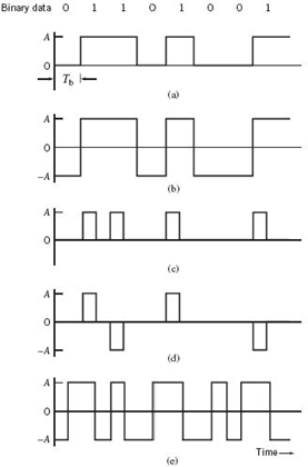
Figure 6.24  Line codes for the electrical representations of binary data: (a) unipolar nonreturn-to-zero (NRZ) signaling; (b) polar NRZ signaling; (c) unipolar return-to-zero (RZ) signaling; (d) bipolar RZ signaling; (e) split-phase or Manchester code.

Figure 6.25  Power spectra of line codes: (a) unipolar NRZ signal; (b) polar NRZ signal; (c) unipolar RZ signal; (d) bipolar RZ signal; (e) Manchester-encoded signal. The frequency is normalized with respect to the bit rate 1/T_b, and the average power is normalized to unity.

 Unipolar NRZ Signaling

In this line code, symbol 1 is represented by transmitting a pulse of amplitude A for the duration of the symbol, and symbol 0 is represented by switching off the pulse, as in Figure 6.24a. The unipolar NRZ line code is also referred to as on–off signaling. Disadvantages of on–off signaling are the waste of power due to the transmitted DC level and the fact that the power spectrum of the transmitted signal does not approach zero at zero frequency.

 Polar NRZ Signaling

In this second line code, symbols 1 and 0 are represented by transmitting pulses of amplitudes +A and –A, respectively, as illustrated in Figure 6.24b. The polar NRZ line code is relatively easy to generate, but its disadvantage is that the power spectrum of the signal is large near zero frequency.

 Unipolar RZ Signaling

In this third line code, symbol 1 is represented by a rectangular pulse of amplitude A and half-symbol width and symbol 0 is represented by transmitting no pulse, as illustrated in Figure 6.24c. An attractive feature of the unipolar RZ line code is the presence of delta functions at f = 0, ±1/T_b in the power spectrum of the transmitted signal; the delta functions can be used for bit-timing recovery at the receiver. However, its disadvantage is that it requires 3 dB more power than polar RZ signaling for the same probability of symbol error.

 Bipolar RZ Signaling

This line code uses three amplitude levels, as indicated in Figure 6.24(d). Specifically, positive and negative pulses of equal amplitude (i.e., +A and –A) are used alternately for symbol 1, with each pulse having a half-symbol width; no pulse is always used for symbol 0. A useful property of the bipolar RZ signaling is that the power spectrum of the transmitted signal has no DC component and relatively insignificant low-frequency components for the case when symbols 1 and 0 occur with equal probability. The bipolar RZ line code is also called alternate mark inversion (AMI) signaling.

 Split-Phase (Manchester Code)

In this final method of signaling, illustrated in Figure 6.24e, symbol 1 is represented by a positive pulse of amplitude A followed by a negative pulse of amplitude –A, with both pulses being half-symbol wide. For symbol 0, the polarities of these two pulses are reversed. A unique property of the Manchester code is that it suppresses the DC component and has relatively insignificant low-frequency components, regardless of the signal statistics. This property is essential in some applications.

6.11  Summary and Discussion

In this chapter we introduced two fundamental and complementary processes:

• Sampling, which operates in the time domain; the sampling process is the link between an analog waveform and its discrete-time representation.
• Quantization, which operates in the amplitude domain; the quantization process is the link between an analog waveform and its discrete-amplitude representation.

The sampling process builds on the sampling theorem, which states that a strictly band-limited signal with no frequency components higher than W Hz is represented uniquely by a sequence of samples taken at a uniform rate equal to or greater than the Nyquist rate of 2W samples per second. The quantization process exploits the fact that any human sense, as ultimate receiver, can only detect finite intensity differences.

The sampling process is basic to the operation of all pulse modulation systems, which may be classified into analog pulse modulation and digital pulse modulation. The distinguishing feature between them is that analog pulse modulation systems maintain a continuous amplitude representation of the message signal, whereas digital pulse modulation systems also employ quantization to provide a representation of the message signal that is discrete in both time and amplitude.

Analog pulse modulation results from varying some parameter of the transmitted pulses, such as amplitude, duration, or position, in which case we speak of PAM, pulse-duration modulation, or pulse-position modulation, respectively. In this chapter we focused on PAM, as it is used in all forms of digital pulse modulation.

Digital pulse modulation systems transmit analog message signals as a sequence of coded pulses, which is made possible through the combined use of sampling and quantization. PCM is an important form of digital pulse modulation that is endowed with some unique system advantages, which, in turn, have made it the standard method of modulation for the transmission of such analog signals as voice and video signals. The advantages of PCM include robustness to noise and interference, efficient regeneration of the coded pulses along the transmission path, and a uniform format for different kinds of baseband signals.

Indeed, it is because of this list of advantages unique to PCM that it has become the method of choice for the construction of public switched telephone networks (PSTNs). In this context, the reader should carefully note that the telephone channel viewed from the PSTN by an Internet service provider, for example, is nonlinear due to the use of companding and, most importantly, it is entirely digital. This observation has a significant impact on the design of high-speed modems for communications between a computer user and server, which will be discussed in Chapter 8.

DM and DPCM are two other useful forms of digital pulse modulation. The principal advantage of DM is the simplicity of its circuitry, which is achieved at the expense of increased transmission bandwidth. In contrast, DPCM employs increased circuit complexity to reduce channel bandwidth. The improvement is achieved by using the idea of prediction to reduce redundant symbols from an incoming data stream. A further improvement in the operation of DPCM can be made through the use of adaptivity to account for statistical variations in the input data. By so doing, bandwidth requirement may be reduced significantly without serious degradation in system performance.⁸

   Problems

     Sampling Process

6.1  In natural sampling, an analog signal g(t) is multiplied by a periodic train of rectangular pulses c(t), each of unit area. Given that the pulse repetition frequency of this periodic train is f_s and the duration of each rectangular pulse is T (with f_sT ≪ 1), do the following:

a. Find the spectrum of the signal s(t) that results from the use of natural sampling; you may assume that time t = 0 corresponds to the midpoint of a rectangular pulse in c(t).

b. Show that the original signal g(t) may be recovered exactly from its naturally sampled version, provided that the conditions embodied in the sampling theorem are satisfied.

6.2  Specify the Nyquist rate and the Nyquist interval for each of the following signals:

a. g(t) = sinc(200t).

b. g(t) = sinc²(200t).

c. g(t) = sinc(200t) + sinc²(200t).

6.3  Discussion of the sampling theorem presented in Section 6.2 was confined to the time domain. Describe how the sampling theorem can be applied in the frequency domain.

Pulse-Amplitude Modulation

6.4  Figure P6.4 shows the idealized spectrum of a message signal m(t). The signal is sampled at a rate equal to 1 kHz using flat-top pulses, with each pulse being of unit amplitude and duration 0.1ms. Determine and sketch the spectrum of the resulting PAM signal.

Figure P6.4

6.5  In this problem, we evaluate the equalization needed for the aperture effect in a PAM system. The operating frequency f = f_s/2, which corresponds to the highest frequency component of the message signal for a sampling rate equal to the Nyquist rate. Plot 1/sinc(0.5T/T_s) versus T/T_s, and hence find the equalization needed when T/T_s = 0.1.

6.6  Consider a PAM wave transmitted through a channel with white Gaussian noise and minimum bandwidth B_T = 1/2T_s, where T_s is the sampling period. The noise is of zero mean and power spectral density N₀/2. The PAM signal uses a standard pulse g(t) with its Fourier transform defined by

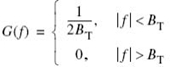
By considering a full-load sinusoidal modulating wave, show that PAM and baseband-signal transmission have equal SNRs for the same average transmitted power.

6.7  Twenty-four voice signals are sampled uniformly and then time-division multiplexed (TDM). The sampling operation uses flat-top samples with 1 μs duration. The multiplexing operation includes provision for synchronization by adding an extra pulse of sufficient amplitude and also 1 μs duration. The highest frequency component of each voice signal is 3.4 kHz.

a. Assuming a sampling rate of 8 kHz, calculate the spacing between successive pulses of the multiplexed signal.

b. Repeat your calculation assuming the use of Nyquist rate sampling.

6.8  Twelve different message signals, each with a bandwidth of 10 kHz, are to be multiplexed and transmitted. Determine the minimum bandwidth required if the multiplexing/modulation method used is time-division multiplexing (TDM), which was discussed in Chapter 1.

Pulse-Code Modulation

6.9  A speech signal has a total duration of 10 s. It is sampled at the rate of 8 kHz and then encoded. The signal-to-(quantization) noise ratio is required to be 40 dB. Calculate the minimum storage capacity needed to accommodate this digitized speech signal.

6.10  Consider a uniform quantizer characterized by the input-output relation illustrated in Figure 6.9a. Assume that a Gaussian-distributed random variable with zero mean and unit variance is applied to this quantizer input.

a. What is the probability that the amplitude of the input lies outside the range –4 to +4?

b. Using the result of part a, show that the output SNR of the quantizer is given by

where R is the number of bits per sample. Specifically, you may assume that the quantizer input extends from –4 to +4. Compare the result of part b with that obtained in Example 2.

6.11  A PCM system uses a uniform quantizer followed by a 7-bit binary encoder. The bit rate of the system is equal to 50 × 10⁶ bits/s.

a. What is the maximum message bandwidth for which the system operates satisfactorily?

b. Determine the output signal-to-(quantization) noise when a full-load sinusoidal modulating wave of frequency 1 MHz is applied to the input.

6.12  Show that with a nonuniform quantizer the mean-square value of the quantization error is approximately equal to , where Δ_i is the ith step size and p_i is the probability that the input signal amplitude lies within the ith interval. Assume that the step size Δ_i is small compared with the excursion of the input signal.

6.13  

a. A sinusoidal signal with an amplitude of 3.25 V is applied to a uniform quantizer of the midtread type whose output takes on the values 0, ±1, ±2, ±3 V. Sketch the waveform of the resulting quantizer output for one complete cycle of the input.

b. Repeat this evaluation for the case when the quantizer is of the midrise type whose output takes on the values 0.5, ±1.5, ±2.5, ±3.5 V.

6.14  The signal

is transmitted using a 40-bit binary PCM system. The quantizer is of the midrise type, with a step size of 1V. Sketch the resulting PCM wave for one complete cycle of the input. Assume a sampling rate of four samples per second, with samples taken at t(s) = ±1/8, ±3/8, ±5/8,…

6.15  Figure P6.15 shows a PCM signal in which the amplitude levels of +1V and –1V are used to represent binary symbols 1 and 0, respectively. The codeword used consists of three bits. Find the sampled version of an analog signal from which this PCM signal is derived.

Figure P6.15

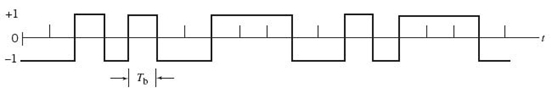
6.16  Consider a chain of (n – 1) regenerative repeaters, with a total of n sequential decisions made on a binary PCM wave, including the final decision made at the receiver. Assume that any binary symbol transmitted through the system has an independent probability p₁ of being inverted by any repeater. Let p_n represent the probability that a binary symbol is in error after transmission through the complete system.

a. Show that

b. If p₁ is very small and n is not too large, what is the corresponding value of p_n?

6.17  Discuss the basic issues involved in the design of a regenerative repeater for PCM.

Linear Prediction

6.18  A one-step linear predictor operates on the sampled version of a sinusoidal signal. The sampling rate is equal to 10f₀, where f₀ is the frequency of the sinusoid. The predictor has a single coefficient denoted by w₁.

a. Determine the optimum value of w₁ required to minimize the prediction-error variance.

b. Determine the minimum value of the prediction error variance.

6.19  A stationary process X(t) has the following values for its autocorrelation function:

a. Calculate the coefficients of an optimum linear predictor involving the use of three unit-time delays.

b. Calculate the variance of the resulting prediction error.

6.20  Repeat the calculations of Problem 6.19, but this time use a linear predictor with two unit-time delays. Compare the performance of this second optimum linear predictor with that considered in Problem 6.19.

Differential Pulse-Code Modulation

6.21  A DPCM system uses a linear predictor with a single tap. The normalized autocorrelation function of the input signal for a lag of one sampling interval is 0.75. The predictor is designed to minimize the prediction-error variance. Determine the processing gain attained by the use of this predictor.

6.22  Calculate the improvement in processing gain of a DPCM system using the optimized three-tap linear predictor. For this calculation, use the autocorrelation function values of the input signal specified in Problem 6.19.

6.23  In this problem, we compare the performance of a DPCM system with that of an ordinary PCM system using companding.

For a sufficiently large number of representation levels, the signal-to-(quantization) noise ratio of PCM systems, in general, is defined by

where 2ⁿ is the number of representation levels. For a companded PCM system using the μ-law, the constant α is itself defined by

For a DPCM system, on the other hand, the constant α lies in the range –3 < α < 15 dBs. The formulas quoted herein apply to telephone-quality speech signals.

Compare the performance of the DPCM system against that of the μ-companded PCM system with μ = 255 for each of the following scenarios:

a. The improvement in (SNR)_O realized by DPCM over companded PCM for the same number of bits per sample.

b. The reduction in the number of bits per sample required by DPCM, compared with the companded PCM for the same (SNR)_O.

6.24  In the DPCM system depicted in Figure P6.24, show that in the absence of channel noise, the transmitting and receiving prediction filters operate on slightly different input signals.

Figure P6.24

6.25  Figure P6.25 depicts the block diagram of adaptive quantization for DPCM. The quantization is of a backward estimation kind because samples of the quantization output and prediction errors are used to continuously derive backward estimates of the variance of the message signal. This estimate computed at time n is denoted by . Given this estimate, the step size is varied so as to match the actual variance of the message sample m_n, as shown by

where is the estimate of the standard deviation and ϕ is a constant. An attractive feature of the adaptive scheme in Figure P6.25 is that samples of the quantization output and the prediction error are used to compute the predictor’s coefficients.

Modify the block diagram of the DPCM transmitter in Figure P6.19a so as to accommodate adaptive prediction with backward estimation.

Figure P6.25

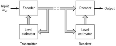
Delta Modulation

6.26  Consider a test signal m(t) defined by a hyperbolic tangent function:

where A and β are constants. Determine the minimum step size Δ for DM of this signal, which is required to avoid slope-overload distortion.

6.27  Consider a sine wave of frequency f_m and amplitude A_m, which is applied to a delta modulator of step size Δ. Show that slope-overload distortion will occur if

where T_s is the sampling period. What is the maximum power that may be transmitted without slope-overload distortion?

6.28  A linear delta modulator is designed to operate on speech signals limited to 3.4 kHz. The specifications of the modulator are as follows:

• Sampling rate = 10f_Nyquist, where f_Nyquist is the Nyquist rate of the speech signal.
• Step size Δ = 100 mV.

The modulator is tested with a 1kHz sinusoidal signal. Determine the maximum amplitude of this test signal required to avoid slope-overload distortion.

6.29  In this problem, we derive an empirical formula for the average signal-to-(quantization) noise ratio of a DM system with a sinusoidal signal of amplitude A and frequency f_m as the test signal. Assume that the power spectral density of the granular noise generated by the system is governed by the formula

where f_s is the sampling rate and Δ is the step size. (Note that this formula is basically the same as that for the power spectral density of quantization noise in a PCM system with Δ/2 for PCM being replaced by Δ for DM.) The DM system is designed to handle analog message signals limited to bandwidth W.

a. Show that the average quantization noise power produced by the system is

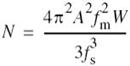
where it is assumed that the step size Δ has been chosen in accordance with the formula used in Problem 6.28 so as to avoid slope-overload distortion.

b. Hence, determine the signal-to-(quantization) noise ratio of the DM system for a sinusoidal input.

6.30  Consider a DM system designed to accommodate analog message signals limited to bandwidth W = 5 kHz. A sinusoidal test signal of amplitude A = 1V and frequency f_m = 1 kHz is applied to the system. The sampling rate of the system is 50 kHz.

a. Calculate the step size Δ required to minimize slope overload distortion.

b. Calculate the signal-to-(quantization) noise ratio of the system for the specified sinusoidal test signal.

For these calculations, use the formula derived in Problem 6.29.

6.31  Consider a low-pass signal with a bandwidth of 3 kHz. A linear DM system with step size Δ = 0.1V is used to process this signal at a sampling rate 10 times the Nyquist rate.

a. Evaluate the maximum amplitude of a test sinusoidal signal of frequency 1kHz, which can be processed by the system without slope-overload distortion.

b. For the specifications given in part a, evaluate the output SNR under (i) prefiltered and (ii) postfiltered conditions.

6.32  In the conventional form of DM, the quantizer input may be viewed as an approximate to the derivative of the incoming message signal m(t). This behavior leads to a drawback of DM: transmission disturbances (e.g., noise) result in an accumulation error in the demodulated signal. This drawback can be overcome by integrating the message signal m(t) prior to DM, resulting in three beneficial effects:

a. Low frequency content of m(t) is pre-emphasized.

b. Correlation between adjacent samples of m(t) is increased, tending to improve overall system performance by reducing the variance of the error signal at the quantizer input.

c. Design of the receiver is simplified.

Such a DM scheme is called delta–sigma modulation.

Construct a block diagram of the delta–sigma modulation system in such a way that it provides an interpretation of the system as a “smoothed” version of 1-bit PCM in the following composite sense:

• smoothness implies that the comparator output is integrated prior to quantization, and
• 1-bit modulation merely restates that the quantizer consists of a hard limiter with only two representation levels.

Explain how the receiver of the delta–sigma modulation system is simplified, compared with conventional DM.

Line Codes

6.33  In this problem, we derive the formulas used to compute the power spectra of Figure 6.25 for the five line codes described in Section 6.10. In the case of each line code, the bit duration is T_b and the pulse amplitude A is conditioned to normalize the average power of the line code to unity as indicated in Figure 6.25. Assume that the data stream is randomly generated and symbols 0 and 1 are equally likely.

Derive the power spectral densities of these line codes as summarized here:

a. Unipolar NRZ signals:

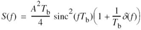
b. Polar NRZ signals:

c. Unipolar RZ signals:

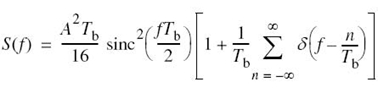
d. Bipolar RZ signals:

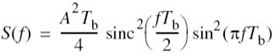
e. Manchester-encoded signals:

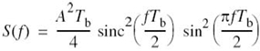
Hence, confirm the spectral plots displayed in Figure 6.25.

6.34  A randomly generated data stream consists of equiprobable binary symbols 0 and 1. It is encoded into a polar NRZ waveform with each binary symbol being defined as follows:

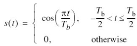
a. Sketch the waveform so generated, assuming that the data stream is 00101110.

b. Derive an expression for the power spectral density of this signal and sketch it.

c. Compare the power spectral density of this random waveform with that defined in part b of Problem 6.33.

6.35  Given the data stream 1110010100, sketch the transmitted sequence of pulses for each of the following line codes:

a. unipolar NRZ

b. polar NRZ

c. unipolar RZ

d. bipolar RZ

e. Manchester code.

Computer Experiments

**6.36  A sinusoidal signal of frequency f₀ = 10⁴/2πHz is sampled at the rate of 8 kHz and then applied to a sample-and-hold circuit to produce a flat-topped PAM signal s(t) with pulse duration T = 500 μs.

a. Compute the waveform of the PAM signal s(t).

b. Compute |S(f)|, denoting the magnitude spectrum of the PAM signal s(t).

c. Compute the envelope of |S(f)|. Hence confirm that the frequency at which this envelope goes through zero for the first time is equal to (1/T) = 20 kHz.

**6.37 In this problem, we use computer simulation to compare the performance of a companded PCM system using the μ-law against that of the corresponding system using a uniform quantizer. The simulation is to be performed for a sinusoidal input signal of varying amplitude.

With a companded PCM system in mind, Table 6.4 describes the 15-segment pseudo-linear characteristic that consists of 15 linear segments configured to approximate the logarithmic μ-law of (6.48), with μ = 255. This approximation is constructed in such a way that the segment endpoints in Table 6.4 lie on the compression curve computed from (6.48).

Table 6.4  The 15-segment companding characteristic (μ = 255)

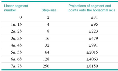
a. Using the μ-law described in Table 6.4, plot the output signal-to-noise ratio as a function of the input signal-to-noise ratio, both ratios being expressed in decibels.

b. Compare the results of your computation in part (a) with a uniform quantizer having 256 representation levels.

**6.38  In this experiment we study the linear adaptive prediction of a signal x_n governed by the following recursion:

where v_n is drawn from a discrete–time white noise process of zero mean and unit variance. (A process generated in this manner is referred to as an autoregressive process of order two.) Specifically, the adaptive prediction is performed using the normalized LMS algorithm defined by

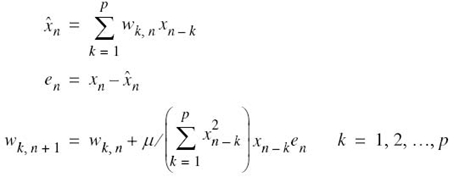
where p is the prediction order and μ is the normalized step-size parameter. The important point to note here is that μ is dimensionless and stability of the algorithm is assured by choosing it in accordance with the formula

The algorithm is initiated by setting

The learning curve of the algorithm is defined as a plot of the mean-square error versus the number of iterations n for specified parameter values, which is obtained by averaging the plot of versus n over a large number of different realizations of the algorithm.

a. Plot the learning curves for the adaptive prediction of x_n for a fixed prediction order p = 5 and three different values of step-size parameter: μ = 0.0075, 0.05, and 0.5.

b. What observations can you make from the learning curves of part a?

**6.39  In this problem, we study adaptive delta modulation, the underlying principle of which is two-fold:

1.  If successive errors are of opposite polarity, then the delta modulator is operating in the granular mode, in which case the step size Δ is reduced.

2.  If, on the other hand, the successive errors are of the same polarity, then the delta modulator is operating in the slope-overload mode, in which case the step size Δ is increased.

Parts a and b of Figure P6.39 depict the block diagrams of the transmitter and receiver of the adaptive delta modulator, respectively, in which the step size, Δ, is increased or decreased by a factor of 50% at each iteration of the adaptive process, as shown by:

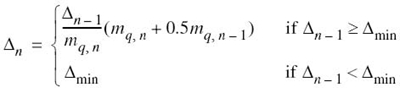
where Δ_n is the step size at iteration (time step) n of the adaptation algorithm, and m_{q, n} is the 1-bit quantizer output that equals ±1.

Specifications: The input signal applied to the transmitter is sinusoidal as shown by

where A = 10 and f_m = f_s /100 where f_s is the sampling frequency; the step size Δ_n = 1 for all n ; Δ_min = 1/8.

a. Using the above-described adaptation algorithm, use a computer to plot the resulting waveform for one complete cycle of the sinusoidal modulating signal, and also display the coded modulator output in the transmitter.

b. For the same specifications, repeat the computation using linear modulation.

c. Comment on the results obtained in parts a and b of the problem.

Figure P6.39

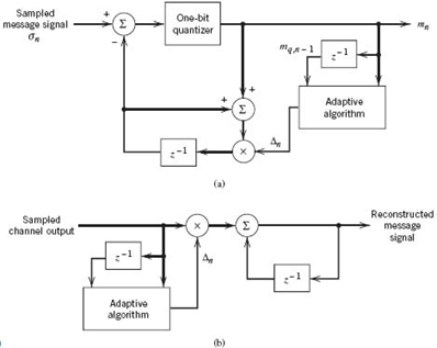
        Notes

1. For an exhaustive study of quantization noise in signal processing and communications, see Widrow and Kollar (2008).

2. The two necessary conditions of (3.42) and (3.47) for optimality of a scalar quantizer were reported independently by Lloyd (1957) and Max (1960), hence the name “Lloyd–Max quantizer.” The derivation of these two optimality conditions presented in this chapter follows the book by Gersho and Gray (1992).

3. The μ-law is used in the USA, Canada, and Japan. On the other hand, in Europe, the A-law is used for signal compression.

4. In actual PCM systems, the companding circuitry does not produce an exact replica of the nonlinear compression curves shown in Figure 6.14. Rather, it provides a piecewise linear approximation to the desired curve. By using a large enough number of linear segments, the approximation can approach the true compression curve very closely; for detailed discussion of this issue, see Bellamy (1991).

5. For a discussion of noise in analog modulation systems with particular reference to FM, see Chapter 4 of Communication Systems (Haykin, 2001).

6. To simplify notational matters, R_M is used to denote the autocorrelation matrix in (6.70) rather than R_MM as in Chapter 4 on Stochastic Processes. To see the rationale for this simplification, the reader is referred to (6.79) for simplicity. For the same reason, henceforth the practice adopted in this chapter will be continued for the rest of the book, dealing with autocorrelation matrices and power spectral density.

7. An optimum predictor that follows (6.77) is said to be a special case of the Wiener filter.

8. For a detailed discussion of adaptive DPCM involving the use of adaptive quantization with forward estimation as well as backward estimation, the reader is referred to the classic book (Jayant and Noll, 1984).