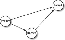
Bayesian networks consist of nodes representing random variables and arcs or links representing the causal relationship between variables. Figure 13-1 shows an example Bayesian network. Imagine a game in which an NPC can encounter a chest that can be locked or unlocked. Whether it is locked depends on whether it contains treasure or whether it is trapped.

Figure 13-1. Example Bayesian network

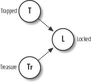
In this example, the nodes labeled T, Tr, and L represent random variables (often referred to as events in the probabilistic sense). The arrows connecting each node represent causal relationships. You can think of nodes at the tail of the arrows as parents and nodes at the head of the arrows as children. Here, parents cause children. For example, Figure 13-1 shows that Locked is caused by Trapped or Treasure or both Trapped and Treasure. You should be aware that this causal relationship is probabilistic and not certain. For example, the chest being Trapped does not necessarily always cause the chest to be Locked. There’s a certain probability that Trapped might cause Locked, but it’s possible that Trapped might not cause Locked.

You measure the strength of the connections between events in terms of probabilities. Each node has an associated conditional probability table that gives the probability of any outcome of the child event given all possible combinations of outcomes of its parents. For our purposes, we’re going to consider discrete events only. What we mean here is that any event, any variable, can take on any one of a set of discrete values. These values are assumed to be mutually exclusive and exhaustive. For example, Locked can take on values of TRUE or FALSE.

Let’s assume that Trapped can be either TRUE or FALSE. Let’s also assume Treasure can be either TRUE or FALSE. If Locked can take on the values TRUE or FALSE, we need a conditional probability table for Locked that gives the probability of Locked being TRUE given every combination of values for Trapped and Treasure, and the probability of Locked being false given every combination of values for Trapped and Treasure. Table 13-1 summarizes the conditional probability table for Locked in this case.

In this table, the first two columns show all combinations of values for Trapped and Treasure. The third column shows the probability that Locked=TRUE given each combination of values for Trapped and Treasure, while the last column shows the probability that Locked=FALSE given each combination of values for Trapped and Treasure. The tilde symbol, ∼, as used here indicates the conjugate of a binary event. If P(T) is the probability of Trapped being equal to TRUE, P(∼T) is the probability of Trapped being equal to FALSE. Note that each of the three events considered here are binary in that they each can take on only one of two values. This yields the 2 × 4 set of conditional probabilities for Locked, as shown in Table 13-1.

As the number of possible values for these events gets larger, or as the number of parent nodes for a given child node goes up, the number of entries in the conditional probability table for the child node increases exponentially. This is one of the biggest deterrents for using Bayesian methods in games. Not only does it become difficult to determine all of these conditional probabilities, but also as the size of the network increases, the computational requirements become prohibitive for real-time games. (Technically Bayesian networks are considered NP-hard, which means they are computationally too expensive for large numbers of nodes.)

Keep in mind that every child node will require a conditional probability table. So-called root nodes, nodes that don’t have parents—events Trapped and Treasure in this example—don’t have conditional probability tables. Instead, they have what are called prior probability tables which contain the probabilities of these events taking on each of their possible values. The term prior used here means that these are probabilities for root nodes before we make adjustments to the probabilities given new information somewhere else in the network. Updated probabilities given new information are called posterior probabilities. We’ll see examples of this sort of calculation later.

The complexity we discussed here is a major incentive for keeping Bayesian networks for use in games simple and specific. For example, theoretically you could construct a Bayesian network to control every aspect of an NPC unit. You could have nodes in the network representing decisions to chase or evade, and still other nodes to represent turn left, turn right, and so on. The trouble with this approach is that the networks become incredibly complex and difficult to set up, solve, and test. Further, the required conditional probability tables become so large that you’d have to resort to some form of training to figure them out rather than specify them. We don’t advocate this approach.

As we mentioned in Chapter 1, and as we’ll discuss in Chapter 14 on neural networks, we recommend that you use Bayesian methods for very specific decision-making problems and leave the other AI tasks to other methods that are better suited for them. Why use a Bayesian network to steer a chasing unit when reliable, easy, and robust deterministic methods are available for that task? Use the Bayesian network to decide whether to chase or evade and let other algorithms take over to handle the actual chasing or evading.

You can make three basic types of reasoning or inference using Bayesian networks. For this discussion, we’ll refer to the simple networks shown in Figure 13-2.

Figure 13-2. Simple networks

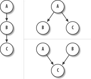
The network on the left is called a causal chain, in this case a three-node chain. The network on the upper right is called a common cause network. It’s also more commonly referred to as a naïve Bayesian network or Bayesian classifier. The network on the lower right is called a common effect network. The three basic types of reasoning are as follows:

The structure on the lower right in Figure 13-2 implies that events A and B are independent of each other. There’s no causal link between A and B. However, if we learn something about C and then something about A or B, we do affect the probability of A or B. In our example, learning that C is true and that B also is true lowers the probability that A is true even though A and B are independent events.

Now consider the network shown on the left in Figure 13-2. In this case, we see that A causes B which in turn causes C. If we learn the state of B, we can make inferences on the state of C irrespective of the state of A. A has no influence on our belief of event C if we know the state of B. In Bayesian lingo, node B blocks A from affecting C.

Another form of independence present in Bayesian networks is d-separation. Look back at the network shown in Figure 13-1. Instead of one node blocking another node, as in the previous discussion, you could have a situation in which a node blocks clusters of nodes. In Figure 13-1, C causes D and D causes E and F, but A and B cause C. However, if we learn the state of C, A and B have no effect on D and thus no effect on E and F. Likewise, if we learn something about the state of D, nodes A, B, and C become irrelevant to E and F. Identifying these independence situations is helpful when trying to solve Bayesian networks because we can treat parts of a network separately, simplifying some computations.

Actually solving, or making inferences, using Bayesian networks involves calculating probabilities using the rules we discussed in Chapter 12. We’re going to show you how to do this for simple networks in the examples that follow. We should point out, though, that some general-purpose methods for solving complex Bayesian networks we aren’t going to cover. These networks include the popular message passing algorithm (see the second reference cited at the end of this chapter) as well as other approximate stochastic methods. Many of these methods don’t seem appropriate for real-time games because computation requirements are large. Here, again, we recommend that you keep Bayesian networks simple if you’re going to use them in games. Of course, you don’t have to listen to us, but by keeping them simple, you can use them where they are best suited for specific tasks and let other methods do their job. This will make your testing and debugging job easier because you can isolate the complicated AI code from the rest of your AI code.

Sometimes it’s helpful to look at problems in the form of tree diagrams as well. The tree diagram for this problem is very simple, as shown in Figure 13-4.

Figure 13-4. Tree diagram

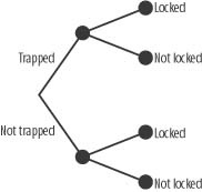
Looking at this tree diagram, it is clear that a chest can be locked in two possible ways and can be unlocked in two possible ways. Each branch in the tree has a corresponding probability associated with it. These are the same probabilities shown in Tables 13-2 and 13-3. This diagram illustrates the compactness of Bayesian network-style graphs as opposed to tree diagrams for visualizing causal relationships. This is important for more complicated problems with greater numbers of events and possible states for each event. In such cases, tree diagrams can become unwieldy in terms of visualizing the relationships between each event.

We can determine the probabilities we need—those shown in Tables 13-2 and 13-3—by gathering statistics during the game. For example, every time an NPC encounters a chest and opens it, the frequencies of the chest being trapped versus not trapped can be updated. The NPC effectively learns these probabilities through experience. You can have each NPC learn based on its own experience, or you can have groups of NPCs learn collectively. You also can collect statistics on the frequencies of chests being locked given they are trapped and locked given they are not trapped to determine the conditional probabilities. Because we are using discrete probabilities and because each event has two states, you’ll have to develop a four-element conditional probability table as we discussed earlier. In a game, it is plausible that any given chest can exist in any one of the four states we illustrated in Figure 13-4. For example, a player can put his valuables in a chest and lock it without trapping it because he might not have the skill or materials required to set traps. Or a player can possess skill and materials to trap the chest as well as lock it, and so on. Therefore, we can’t assume that a chest always will be trapped or always will be locked, and so forth.

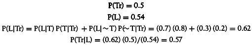
In this example, we’re going to use diagnostic inference. What we aim to do is answer the question, given an NPC encounters a chest what is the probability that the chest is trapped? If the NPC does not observe that the chest is locked, the probability that the chest is trapped is simply p _T. However, if the NPC observes the state of the chest being locked, we can revise the probability of the chest being trapped given this new information. We’ll use Bayes’ rule to make this revision. Bayes’ rule yields the following:

Here P(T) represents the probability that Trapped=TRUE, P(L) represents the probability of Locked=TRUE, and P(L|T) represents the probability that Locked=TRUE given that Trapped=TRUE. In English, Bayes’ rule for this problem says that the probability that the chest is trapped given that the chest is locked is equal to the probability that the chest is locked given that it is trapped times the probability that the chest is trapped divided by the probability that the chest is locked. P(L|T) is taken from the conditional probability table. P(T) also is known from the probability table. However, we must calculate P(L)—the probability that the chest is locked. Looking at the tree diagram in Figure 13-4, we see that the chest can be locked in two ways: 1) given the chest is trapped; or 2) given the chest is not trapped. We can use probability rule 4 from Chapter 12 to determine P(L). In this case, P(L) is as follows:

Again, in words, this says that the probability of the chest being locked is equal to the probability of the chest being locked given that it is trapped times the probability of the chest being trapped plus the probability of the chest being locked given that it is not trapped times the probability of the chest being not trapped. Here the tilde symbol, ∼, indicates the conjugate state. For example, if P(T) represents the probability that the event Trapped=TRUE, P(∼T) represents the probability that the event Trapped=FALSE.

Notice that we use rule 6 from Chapter 12 to determine the probability of Locked=TRUE and Trapped=TRUE—that is, P(L|T) P(T). The same rule applies when determining the probability of Locked=TRUE and Trapped=FALSE—that is, P(L|∼T) P(∼T). This also is the conditional probability formula we saw in Chapter 12 in the section “Conditional Probability.”

Let’s consider some real numbers now. Say a given NPC in your game has experience opening 100 chests and of those 100 chests 37 were trapped. Of the 37 trapped chests, 29 were locked. Of the 63 chests that were not trapped, 18 were locked. With this information we can calculate the following probabilities:

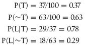
Given these probabilities, we can see that there’s a 37% chance that a given chest is trapped. Now, if the NPC also notices that the chest is locked—that is, Locked=TRUE—the probability that the chest is trapped is revised as follows:

Thus, the observation that the chest is indeed locked increases the NPC’s belief that the chest is trapped. In this case, P(T) goes from 37% to 61%. In Bayesian network lingo, the 37% probability is the prior probability, while the revised probability of 61% is the posterior probability.

Now suppose the NPC observes that the chest was not locked. In this case, we have:

where:

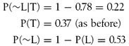
therefore:

This implies that the chest is less likely to be trapped because the NPC was able to observe that it was unlocked.

Now that you have these probabilities, how can your NPC use them to decide whether to open the chest? Let’s go back to the first scenario in which the NPC observed that the chest was locked and the posterior probability of the chest being trapped was determined to be 0.61. Does 61% imply a high probability that the chest is trapped, or perhaps a moderate probability, or maybe even a low probability? We could set up some Boolean logic if-then rules to decide, but clearly this is a good job for fuzzy rules, as we discussed in detail in Chapter 10.

We can set up fuzzy membership functions such as the ones shown in Figure 13-5 for the probability that the chest is trapped.

Figure 13-5. Trapped membership functions

Then we can use fuzzy rules to determine what to do. For example, we can have rules to account for conditions and actions such as the following:

Even better, however, is to consider other relevant information as well. For example, presumably a trapped chest causes some damage to the NPC if it is triggered; therefore, it seems reasonable to consider the NPC’s health in his decision as to whether to open the chest given his belief that it is trapped. Taking this approach, we can set up rules such as the following:

These are just a few examples of the sort of rules you can set up. The benefit of using this Bayesian approach in conjunction with fuzzy rules is that you can give the NPCs the ability to make rational decisions without having to cheat. Further, you give them the ability to make decisions in the face of uncertainty. Moreover, NPCs can adapt to players’ actions using this approach. For example, initially players can lock their chests without trapping them. However, proficient thief NPCs might learn to loot aggressively given the low risk of being hurt while opening a chest. If players start trapping their chests, NPCs can adapt to be less aggressive at looting and more selective as to which chests they open. Further, players might attempt to bluff NPCs by locking chests but not trapping them, or vice versa, and the NPC will adapt accordingly. This brings up another possibility: what if players try to fool NPCs by locking and trapping chests without putting anything of value in the chests? Players might do this to weaken NPCs before attacking them. Because stealing loot is the incentive for opening a chest, it would be cool to allow NPCs to assess the likelihood of the chest being trapped and it containing loot. NPCs could take both factors into account before deciding to open a chest. We’ll consider this case in the next example.

We should point out that the model shown in Figure 13-6 is a simplified model. It is plausible that a chest can be locked given that it contains treasure independent of whether the chest is trapped. This implies a causal link from the Treasure node to the Locked node as well. This is illustrated in Figure 13-7.

Figure 13-7. Alternative model

In this alternative case, you also have to set up conditional probabilities of the chest being locked given the various states of it containing treasure. Although you easily can do this and still solve the network by hand calculations, we’re going to stick with the simple model in our discussion.

We’re going to stick with the model shown in Figure 13-6 for the remainder of this example. To determine the probability that the chest is trapped given it is locked, we proceed in a manner similar to the previous example. However, now we have conditional probabilities for the Trapped event—namely, the probabilities that the chest is trapped given that it contains treasure and that it does not contain treasure. With this in mind, we apply Bayes’ rule as follows:

P(L|T), the probability that the chest is locked given it is trapped, comes from the conditional probability table for the Locked event. This time, however, P(T) is not given, but we can calculate it as follows:

In words, the probability of the chest being trapped is equal to the probability of it being trapped given it contains treasure plus the probability it is trapped given it does not contain treasure. Now, P(L) is as follows:

We’ve already calculated P(T), and P(∼T) is simply 1-P(T), so all we need to do now is look up P(L|T) and P(L|∼T) in the conditional probability table for Locked to determine P(L). Then we can substitute these values in Bayes’ rule to determine P(T |L).

To find the probability of treasure given that the chest is locked, we need to apply Bayes’ rule again as follows:

Notice, however, that Locked is blocked from Treasure given Trapped. Therefore, we can write P(L|Tr) as follows:

This is the case because our simple model assumes that a trapped chest causes a locked chest.

We’ve already calculated P(L) from the previous step, and P(Tr) is given, so we have everything we need to determine P(Tr |L).

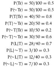
Let’s consider some numbers now. Say a given NPC in your game has experience opening 100 chests, and of those, 50 of them contained treasure. Out of these 50, 40 of them were trapped and of these 40 trapped chests, 28 were locked. Now, of the 10 untrapped chests, three were locked. Further, of the 50 chests containing no treasure, 20 were trapped. With this information, we can calculate the following probabilities:

Let’s assume your NPC approaches a chest. Without observing whether the chest is locked, the NPC would believe that there’s a 50% chance that the chest contained treasure. Now let’s assume the NPC observes that the chest is locked. What is the probability that the chest is trapped and what is the probability that it contains treasure? We can use the formulas shown earlier to determine these probabilities. In this case, we have:

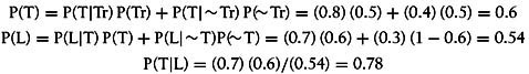
Now we can find P(Tr |L) as follows:

In this example, we see that the observation of the chest being locked raises the probability of the chest being trapped from 60% to 78%. Further, the probability of the chest containing treasure is raised from 50% to 57%.

With this information, you can use fuzzy logic in a manner similar to the previous example to decide for the NPC whether to open the chest. For example, you can set up fuzzy membership functions for the events that the chest is trapped and has treasure and then construct a set of rules along these lines:

These are just a couple of the cases you’d probably want to include in your rules set. Using this approach, your NPC can make decisions considering several factors, even in the face of uncertainty.

The Bayesian network for this simple example looks like that shown in Figure 13-8.

Figure 13-8. Attack mode network

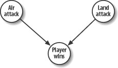
Notice that we have two causes for the player-winning result: air and land attacks. We assume these events are not mutually exclusive—that is, the player can make a land attack, or an air attack, or both. Each event node can take on one of two values: true or false. For example, Air Attack could be true or false,Land Attack could be true or false, and so on.

If instead we allowed only a land or air attack but not both, the network would look like that shown in Figure 13-9.

Figure 13-9. Alternative attack network

In this case, Attack Mode could take on values such as Air Attack or Land Attack. Here, the values are mutually exclusive. For this discussion, we’ll stick with the more general case shown earlier.

As we mentioned earlier, we’ll have to collect some statistics to estimate the probabilities we’re going to need for our inference calculations. The statistics we need to collect as the game is played over and over are as follows:

We can use this data to calculate the following probabilities:

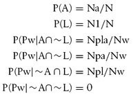
The first two probabilities are the probabilities that the player launches an air attack and the player launches a land attack, respectively. The last four probabilities are conditional probabilities that the player wins the game given all combinations of the Air Attack and Land Attack events. In these formulas, L represents Land Attack, A represents Air Attack, and Pw represents Player Wins. Note also that we assume the probability of the player winning a game is 0 if he does not launch any attack.

With this information, we can determine the probability of the player winning a new game. To do this, we sum the probabilities of all the ways in which a player can win. In this case, the player can win in any of four different ways. These calculations use the joint probability formula for each scenario. The formula is as follows:

The possible ways in which the player can win are summarized in Table 13-7, along with all relevant probability data.

This table looks a little complicated, but it’s really fairly straightforward. The first two columns represent the possible combinations of state for Air Attack and Land Attack. The first column contains the probabilities for each state of Air Attack—true or false—while the second column contains the probabilities for each state of Land Attack—true or false. The third column shows the conditional probability that Player Wins = TRUE given each combination of states for Air Attack and Land Attack. The fourth column, P(Pw), represents the joint probability of the events Air Attack, Land Attack, and Player Wins. You find each entry in this column by simply multiplying the values contained in the first three columns and placing the product in the fourth column. Summing the entries in the fourth column yields the marginal probability of the player winning.

Take a look at the fifth column. The fifth column contains the normalized probabilities for Player Wins. You find the entries in this column by dividing each entry in the fourth column by the sum of the entries in the fourth column. This makes the sum of all the entries in the fifth column add up to 1. (It’s like normalizing a vector to make a vector of unit length.) The results contained in the fifth column basically tell us which combination of states of Air Attack and Land Attack is most likely given that the player wins.

Let’s consider some numbers. We’ll assume we have enough statistics to generate the probabilities shown in the first three columns of Table 13-8.

These numbers indicate that the player wins about 27% of the games played. (This is taken from the sum of the fourth column.) Also, inspection of the fifth column indicates that if the player wins, the most probable mode of attack is an air attack without a land attack. Thus, it would be prudent in this example for the computer to give priority to its air defense systems and to target the player’s aircraft construction resources.

Now let’s assume that for a new game, the player will attack by air and we want to find the probability that he will win in this case. Our probability table now looks like that shown in Table 13-9.

All we’ve done here is replace P(A) by 1.0 and P(∼A) by 0.0 and recalculate the fourth and fifth columns. In this case, we get a new marginal probability that the player wins reflecting our assumption that the player attacks by air. Here, we see the probability that the player wins increases to 37%. Moreover, we see that if the player wins, there’s an 82% chance he won by launching an air attack. This further reinforces our conclusion earlier that the computer should give priority to air defenses and target the player’s air offensive resources. We can make further what-if scenarios if we want. We can, for example, set P(L) to 1.0 and get a new P(Pw) corresponding to an assumed land attack, and so on.

The Bayesian network we’re going to use for this example is shown in Figure 13-10.

Figure 13-10. Strike network

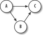
In this model, we call the first strike in the combination event A, the second strike event B, and the third strike event C. We assume that the second strike thrown, event B, in any combination is dependent on the first strike thrown, event A. Further, we assume that the third strike thrown, event C, is dependant on both the first and second strikes thrown, events A and B. Combinations can be anything—punch, punch, high kick; or low kick, low kick, high kick; and so on.

Ordinarily we would need to calculate probabilities for A and conditional probabilities for B given A, and conditional probabilities for C given A and B. However, in this example we’re always going to observe A and B rendering their prior probabilities irrelevant. Therefore, we need only calculate conditional probabilities for C given every combination of A and B. Because three states exist for each strike event A and B, we’ll have to track nine possible combinations of A and B.

We’ll again take a frequency approach to determining these conditional probabilities. After every strike thrown by the player, we’ll increment a counter for that strike given the two prior strikes thrown. We’ll end up with a conditional probability table that looks like the one shown in Table 13-10.

This table shows the probability of strike C taking on each of the three values—punch, low kick, or high kick—given every combination of strikes thrown in A and B. The probabilities shown here are subscripted with indices indicating rows and columns to a lookup matrix. We’re going to use these indices in the example code we’ll present shortly.

To calculate these probabilities, we need to keep track of the total number of strikes thrown. We then can calculate probabilities such as these:

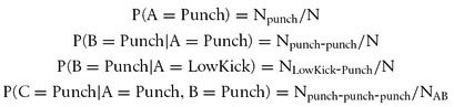
These are just a few examples; we can calculate all the conditional probabilities in this manner. In these equations, N represents the number of strikes thrown and N with a subscript represents the number of a particular strike thrown given previously thrown strikes. For example, N _{punch-punch-punch} is the number of times A, B, and C all equal punch.

In practice you don’t have to store probabilities; the frequencies are sufficient to use to calculate probabilities when required. In this case, we’ll store the frequencies of strike combinations in a 9 × 3 matrix. This matrix will represent counters for all outcomes of C corresponding to all nine combinations of A and B. We’ll also need a nine-element array to store counters for all nine combinations of A and B.

Now, to make a prediction for the next strike, C, look at which two strikes, A and B, were thrown most recently and then look up the combination in the conditional probability table for C. Basically, use A and B to establish which row to consider in the conditional probability matrix, and then simply pick the strike for C that has the highest probability. That is, pick the column with the highest conditional probability.

We’ve put together a little example program to test this approach. We have a window with three buttons on it corresponding to punch, low kick, and high kick. The user can press these in any order to simulate fighting moves. As he throws these strikes, the conditional probabilities we discussed earlier are updated and a prediction for the next strike to be thrown is made. Example 13-1 shows the core function that performs the calculations for this program.

TStrikes ProcessMove(TStrikes move)
{
          int     i, j;
          N++;
          if(move == Prediction) NSuccess++;
          if((AB[0] == Punch) && (AB[1] == Punch)) i = 0;
          if((AB[0] == Punch) && (AB[1] == LowKick)) i = 1;
          if((AB[0] == Punch) && (AB[1] == HighKick)) i = 2;
          if((AB[0] == LowKick) && (AB[1] == Punch)) i = 3;
          if((AB[0] == LowKick) && (AB[1] == LowKick)) i = 4;
          if((AB[0] == LowKick) && (AB[1] == HighKick)) i = 5;
          if((AB[0] == HighKick) && (AB[1] == Punch)) i = 6;
          if((AB[0] == HighKick) && (AB[1] == LowKick)) i = 7;
          if((AB[0] == HighKick) && (AB[1] == HighKick)) i = 8;
          if(move == Punch) j = 0;
          if(move == LowKick) j = 1;
          if(move == HighKick) j = 2;
          NAB[i]++;
          NCAB[i][j]++;
          AB[0] = AB[1];
          AB[1] = move;
          if((AB[0] == Punch) && (AB[1] == Punch)) i = 0;
          if((AB[0] == Punch) && (AB[1] == LowKick)) i = 1;
          if((AB[0] == Punch) && (AB[1] == HighKick)) i = 2;
          if((AB[0] == LowKick) && (AB[1] == Punch)) i = 3;
          if((AB[0] == LowKick) && (AB[1] == LowKick)) i = 4;
          if((AB[0] == LowKick) && (AB[1] == HighKick)) i = 5;
          if((AB[0] == HighKick) && (AB[1] == Punch)) i = 6;
          if((AB[0] == HighKick) && (AB[1] == LowKick)) i = 7;
          if((AB[0] == HighKick) && (AB[1] == HighKick)) i = 8;
          ProbPunch = (double) NCAB[i][0] / (double) NAB[i];
          ProbLowKick = (double) NCAB[i][1] / (double) NAB[i];
          ProbHighKick = (double) NCAB[i][2] / (double) NAB[i];
          if((ProbPunch > ProbLowKick) &&
              (ProbPunch > ProbHighKick))
                return Punch;
          if((ProbLowKick > ProbPunch) &&
             (ProbLowKick > ProbHighKick))
                return LowKick;
          if((ProbHighKick > ProbPunch) &&
              (ProbHighKick > ProbLowKick))
                return HighKick;
          return (TStrikes) rand() % 3; // Last resort
}

This function takes a TStrikes variable called move as a single parameter. TStrikes is simply an enumerated type defined as shown in Example 13-2.

enum TStrikes {Punch, LowKick, HighKick};

The move parameter represents the most recent strike thrown by the player. The ProcessMove function also returns a value of type TStrikes representing the predicted next strike to be thrown by the player.

        int              NAB[9];
        int              NCAB[9][3];
        TStrikes         AB[2];
        double           ProbPunch;
        double           ProbLowKick;
        double           ProbHighKick;
        TStrikes         Prediction;
        TStrikes         RandomPrediction;
        int              N;
        int              NSuccess;