
Chapter 10. Assembly of Forces
Coping with Large Volumes of Data
Thenne entryd in to the bataylle Iubance a geaunt and fought and slewe doune ryght and distressyd many of our knyghtes.
—Sir Thomas Malory (d.1471) Le Morte D’Arthur, V, 11
This chapter deals with the particular challenges that are facing us when data volumes swell. Those challenges include searching gigantic tables effectively, but also avoiding the sometimes distressing performance impact of even a moderate volume increase. We’ll first look at the impact of data growth and a very large number of rows on SQL queries in the general case. Then we’ll examine what happens in the particular environments of data warehousing and decision-support systems.
Increasing Volumes
Some applications see the volume of data they handle increase in considerable proportion over time. In particular, any application that requires keeping online, for regulatory or business analysis purposes, several months or even years of mostly inactive data, often passes through phases of crisis when (mostly) batch programs tend to overshoot the time allocated to them and interfere with regular, human activity.
When you start a new project, the volume of data usually changes, as shown in Figure 10-1. Initially, hardly anything other than a relatively small amount of reference data is loaded into the database. As a new system replaces an older one, data inherited from the legacy system is painfully loaded into the new one. First, because of the radical rethink of the application, conversion from the old system to the new system is fraught with difficulties. When deadlines have to be met and some noncritical tasks have to be postponed, the recovery of legacy data is a prime candidate for slipping behind schedule. As a result, this recovery goes on for some time after the system has become operational and teething problems have been solved. Second, the old system is usually much poorer from a functional perspective than the new one (otherwise, the cost of the new project would have made for difficult acceptance up the food chain). All this means that the volume of prehistoric data will be rather small compared to the data handled by the new system, and several months’ worth of old data will probably be equivalent to a few weeks of new data at most.
Meanwhile, operational data accumulates.
Usually, one encounters the first serious performance issues about midway before the volume that the database is expected to hold at cruising speed. Bad queries and bad algorithms are almost invisible, from an end-user perspective, when volumes are low or moderate. The raw power of hardware often hides gigantic mistakes and may give comfortable sub-second response times for full scans of tables that contain several hundreds of thousands of rows. You may be seriously misusing the hardware, balancing gross programming mistakes with power—but nobody will see that until your volume becomes respectable.
At the first crisis point of the project, “expert tuning” is usually required to add a couple of indexes that should have been there from the start. The system then wobbles until it
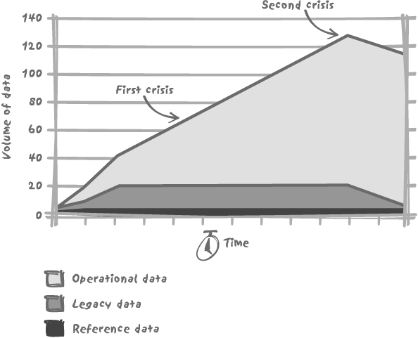
reaches the target volume. There are usually two target volumes: a nominal one (which has been grossly overestimated and which is the volume the system has officially been designed to manage) and the real target volume (which the system just manages to handle and which is often exceeded at some point because archiving of older data has been relegated to the very last lot in the project). The second and more serious crisis often comes in the wake of reaching that point. When archival has finally been put into production, architectural weaknesses reviewed, and some critical processes vigorously rewritten, the system finally reaches cruising speed, with an increase of data related to the natural growth of business—a growth that can lie anywhere between flatness and exponential exuberance.
This presentation of the early months in the life of a new database application is partly caricature; but it probably bears more resemblance to reality than it often should, because the simple mistakes that lead to this caricature are not often avoided. However rigorously one tries to work, errors are made, because of pressure, lack of time for adequate testing, and ambiguous specifications. The only errors that can bring irredeemable failure are those linked to the design of the database and to the choice of the global architecture—two topics that are closely related and that are the foundation of a system. If the foundation is not sturdy enough, you need to pull the whole building down before reconstructing. Other mistakes may require a more or less deep overhaul of what is in place. Most crises, however, need not happen. You must anticipate volume increases when coding. And you must quickly identify and rewrite a query that deteriorates in performance too quickly in the face of increasing data volumes.
Sensitivity of Operations to Volume Increases
All SQL operations are not equally susceptible to variations in performance when the number of rows to be processed increases. Some SQL operations are insensitive to volume increases, some see performance decrease linearly with volume, and some perform very badly with large volumes of data.
Insensitivity to volume increase
Typically, there will be no noticeable difference in a search on the primary key, whether you are looking for one particular key among 1,000 or one among 1,000,000. The common B-tree indexes are rather flat and efficient structures, and the size of the underlying table doesn’t matter for a single-row, primary-key search.
But insensitivity to volume increase doesn’t mean that single primary-key searches are the ultimate SQL search method. When you are looking for a large number of rows, the “transactional” single-row operation can be significantly inefficient. Just consider the following, somewhat artificial, Oracle examples, each showing a range scan on a sequence-generated primary key:
SQL>declare2n_id number;3cursor c is select customer_id4from orders5where order_id between 10000 and 20000;6begin7open c;8loop9fetch c into n_id;10exit when c%notfound;11end loop;12close c;13end;14/
PL/SQL procedure successfully completed.
Elapsed: 00:00:00.27
SQL>declare2n_id number;3begin4for i in 10000 .. 200005loop6select customer_id7into n_id8from orders9where order_id = i;10end loop;11end;12/PL/SQL procedure successfully completed. Elapsed: 00:00:00.63
The cursor in the first example, which does an explicit range
scan, runs twice as fast as the iteration on a single row. Why?
There are multiple technical reasons (“soft parsing,” a fast
acknowledgement at each iteration that the DBMS engine has already
met this statement and knows how to execute it, is one of them), but
the single most important one is that in the first example the
B-tree is descended once, and then the ordered list of keys is
scanned and row addresses found and used to access the table; while
in the second example, the B-tree is descended for each searched
value in the order_id column. The
most efficient way to process a large number of rows is
not to iterate and apply the single-row
process.
Linear sensitivity to volume increases
End users usually understand well that if twice as
many rows are returned, a query will take more time to run; but many
SQL operations double in time when operating on double the number of
rows without the underlying work being as obvious to the end user,
as in the case of a full table scan returning rows one after the
other. Consider the case of aggregate functions; if you compute a
max( ), that aggregation will
always return a single row, but the number of rows the DBMS will
have to operate on may vary wildly over the life of the application.
Perfectly understandable, but end users will always see a single-row
returned, so they may complain of performance degradation over time.
The only way to ensure that the situation will not go from bad to
worse is to put an upper bound on the number of
rows processed by using another criterion such as a date range.
Placing an upper bound keeps data volumes under control. In the case
of max( ), the idea might be to
look for the maximum since a given date, and not necessarily since
the beginning of time. Adding a criterion to a query is not a simple
technical issue and definitely depends on business requirements, but
limiting the scope of queries is an option that certainly deserves
to be pointed out to, and debated with, the people who draft
specifications.
Non-linear sensitivity to volume increases
Operations that perform sorts suffer more from volume increases than operations that just perform a scan, because sorts are complex and require on average a little more than a single pass. Sorting 100 randomly ordered rows is not 10 times costlier than sorting 10 rows, but about 20 times costlier—and sorting 1,000 rows is, on average, something like 300 times costlier than sorting 10 rows.
In real life, however, rows are rarely randomly stored, even when techniques such as clustering indexes (Chapter 5) are not used. A DBMS can sometimes use sorted indexes for retrieving rows in the expected order instead of sorting rows after having fetched them, and performance degradation resulting from retrieving a larger sorted set, although real, is rarely shocking. Be careful though. Performance degradation from sorts often proceeds by fits and starts, because smaller sorts will be fully executed in memory, while larger sorts will result from the merge of several sorted subsets that have each been processed in memory before being written to temporary storage. There are, therefore, some “dangerous surroundings” where one switches from a relatively fast full-memory mode to a much slower memory-plus-temporary-storage mode. Adjusting the amount of memory allocated to sorts is a frequent and efficient tuning technique to improve sort-heavy operations when flirting with the dangerous limit.
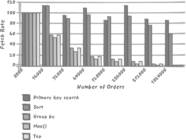
By way of example, Figure 10-2 shows how the fetch rate (number of rows fetched per unit of time) of a number of queries evolves as a table grows. The table used in the test is a very simple orders table defined as follows:
order_idbigint(20) (primary key) customer_id bigint(20) order_date datetime order_shipping char(1) order_comment varchar(50)
The queries are first a simple primary key-based search:
    select order_date
    from orders
    where order_id = ?
then a simple sort:
    select customer_id
    from orders
    order by order_date
then a grouping:
    select customer_id, count(*)
    from orders
    group by customer_id
    having count(*) > 3
then the selection of the maximum value in a nonindexed column:
    select max(order_date)
    from orders
and finally, the selection of the “top 5” customers by number of orders:
    select customer_id
    from (select customer_id, count(*)
          from orders
          group by customer_id
          order by 2 desc) as sorted_customers
    limit 5
(SQL Server would replace the closing limit 5 with an opening select top 5, and Oracle would replace
limit 5 with where rownum <= 5.)
The number of rows in the table has varied between 8,000 and
around 1,000,000, while the number of distinct customer_id values remained constant at
about 3,000. As you can see in Figure 10-2, the primary key
search performs almost as well with one million rows as with 8,000.
There seems to be some very slight degradation at the higher number,
but the query is so fast that the degradation is hardly noticeable.
By contrast, the sort suffers. The performance (measured by rows
returned by unit of time, and therefore independent of the actual
number of rows fetched) of the sorting query decreases by 40% when
the number of rows goes from 8,000 to over one million.
The degradation of performance, though, is even more noticeable for all the queries that, while returning the very same number of aggregated rows, have a great deal more rows to visit to get the relatively few rows to be returned. These queries are typically the type of queries that are going to draw the most complaints from end users. Note that the DBMS doesn’t perform that badly: the performance decrease is very close to proportional to the number of rows, even for the two queries that require a sort (the queries labeled “Group by” and “Top” in Figure 10-2). But end users simply see the same amount of data—just returned much more slowly.
Putting it all together
The main difficulty in estimating how a query will
behave when data volumes increase is that high sensitivity to volume
may be hidden deep inside the query. Typically, a query that finds
the “current value” of an item by running a subquery that looks for
the last time the price was changed, and then performs a max( ) over the price history, is highly
sensitive. If we accumulate a large number of price changes, we
shall probably suffer a slow performance degradation of the
subquery, and by extension of the outer query as well. The
degradation will be much less sensitive with an uncorrelated
subquery, executed only once, than with a correlated subquery that
will compound the effect by its being fired each time it is
evaluated. Such degradation may be barely perceptible in a
single-item operation, but will be much more so in batch
programs.
Note
The situation will be totally different if we are tracking,
for instance, the current status of orders in a merchant system,
because max( ) will apply to a
narrow number of possible states. Even if the number of orders
doubles, max( ) will in that
case always operate on about the same number of rows for one
order.
Another issue is sorts. We have seen that an increase in the number of rows sorted leads to a quite perceptible degradation of performance. Actually, what matters is not so much the number of rows proper as the number of bytes—in other words, the total amount of data to be sorted. This is why joins with what is mostly informational data, such as user-friendly labels associated with an obscure code (as opposed to the data involved in the filtering conditions driving the query), should be postponed to the very last stage of a query.
Let’s take a simple example showing why some joins should be
delayed until the end of a query. Getting the names and addresses of
our 10 biggest customers for the past year will require joining the
orders and order_detail tables to get the amount
ordered by each customer, and joining to a customers table to get each customer’s
details. If we only want to get our 10 biggest customers, we must
get everybody who has bought something from us in the past year,
sort them by decreasing amount, and then limit the output to the
first ten resulting rows. If we join all the information from the
start, we will have to sort the names and addresses of
all our customers from the past year. We don’t
need to operate on such a large amount of data. What we must do is
keep the amount of data to be sorted to the strict minimum—the
customer identifier and the amount. Once everything is sorted, we
can join the 10 customer_ids we
are left with to the customers
table to return all the information that is required. In other
words, we mustn’t write something like:
    select *
    from (select c.customer_name,
                 c.customer_address,
                 c.customer_postal_code,
                 c.customer_state,
                 c.customer_country
                 sum(d.amount)
          from customers c,
               orders_o,
               order_detail d
          where c.customer_id = o.customer_id
            and o.order_date >= some date expression
            and o.order_id = d.order_id
          group by c.customer_name,
                   c.customer_address,
                   c.customer_postal_code,
                   c.customer_state,
                   c.customer_country
           order by 6 desc) as A
    limit 10
but rather something like:
    select c.customer_name,
           c.customer_address,
           c.customer_postal_code,
           c.customer_state,
           c.customer_country
           b.amount
    from (select a.customer_id,
                 a.amount
          from (select o.customer_id,
                       sum(d.amount) as amount
                from orders_o,
                      order_detail d
                where o.order_date >= some date expression
                  and o.order_id = d.order_id
                group by o.customer_id
                order by 2 desc) as a
          limit 10) as b,
          customers c
    where c.customer_id = b.customer_id
    order by b.amount desc
The second sort is a safeguard in case the join modifies the order of the rows resulting from the inner subquery (remember that relational theory knows nothing about sorts and that the DBMS engine is perfectly entitled to process the join as the optimizer finds most efficient). We have two sorts instead of one, but the inner sort operates on “narrower” rows, while the outer one operates on only 10 rows.
Remember what was said in Chapter 4: we must limit the “thickness” of the non-relational layer of SQL queries. The thickness depends on the number and complexity of operations, but also on the amount of data involved. Since sorts and limits of all kinds are non-relational operations, the optimizer will probably not rewrite a query to execute a join after having cut the number of customer identifiers to the bare minimum. Although an attentive reading of two queries may make it obvious that they will return the same result, mathematically proving that they always return the same result borders on mission impossible. An optimizer always plays it safe; a DBMS cannot afford to return wrong results by attempting daring rewrites, especially since it knows hardly anything about semantics. Our example is therefore a case in which the optimizer will limit its action to perform the join in inner queries as efficiently as possible. But ordering and aggregates put a stop to mingling inner and outer queries, and therefore the query will for the most part run as it is written. The query that performs the sort of amounts before the joins is, no doubt, very ugly. But this ugly SQL code is the way to write it, because it is the way the SQL engine should execute it if we want resilience to a strong increase in the number of customers and orders.
Disentangling subqueries
As I have said more than once, correlated subqueries must be fired for each row that requires their evaluation. They are often a major issue when volume increases transform a few shots into sustained rounds of fire. In this section, a real-life example will illustrate both how ill-used correlated subqueries can bog a process down and how one can attempt to save such a situation.
The issue at hand, in an Oracle context, is a query that belongs to an hourly batch to update a security management table. Note that this mechanism is already in itself a fudge to speed up security clearance checks on the system in question. Over time, the process takes more and more time, until reaching, on the production server, 15 minutes—which for an hourly process that suspends application availability is a bit too much. The situation sends all bells ringing and all whistles blowing. Red alert!
The slowness of the process has been narrowed down to the following statement:
    insert /*+ append */ into fast_scrty
     ( emplid,
       rowsecclass,
       access_cd,
       empl_rcd,
       name,
       last_name_srch,
       setid_dept,
       deptid,
       name_ac,
       per_status,
       scrty_ovrd_type)
    select distinct
           emplid,
           rowsecclass,
           access_cd,
           empl_rcd,
           name,
           last_name_srch,
           setid_dept,
           deptid,
           name_ac,
           per_status,
          'N'
    from pers_search_fast
Statistics are up to date, so we must focus our attack on the
query. As it happens, the ill-named pers_search_fast is a view defined by the
following query:
    1 select a.emplid,
    2        sec.rowsecclass,
    3        sec.access_cd,
    4        job.empl_rcd,
    5        b.name,
    6        b.last_name_srch,
    7        job.setid_dept,
    8        job.deptid,
    9        b.name_ac,
    10        a.per_status
    11 from person a,
    12      person_name b,
    13      job,
    14      scrty_tbl_dept sec
    15 where a.emplid = b.emplid
    16   and b.emplid = job.emplid
    17   and (job.effdt=
    18          ( select max(job2.effdt)
    19            from job job2
    20            where job.emplid = job2.emplid
    21              and job.empl-rcd = job2.empl_rcd
    22              and job2.effdt <= to_date(to_char(sysdate,
    23                                               'YYYY-MM-DD'),'YYYY-MM-DD'))
    24        and job.effseq =
    25              ( select max(job3.effseq)
    26                from job job3
    27                where job.emplid = job3.emplid
    28                  and job.empl_rcd = job3.empl_rcd
    29                  and job.effdt = job3.effdt ) )
    30   and sec.access_cd = 'Y'
    31   and exists
    32           ( select 'X'
    33             from treenode tn
    34             where tn.setid = sec.setid
    35               and tn.setid = job.setid_dept
    36               and tn.tree_name = 'DEPT_SECURITY'
    37               and tn.effdt = sec.tree_effdt
    38               and tn.tree_node = job.deptid
    39               and tn.tree_node_num between sec.tree_node_num
    40                                        and sec.tree_node_num_end
    41               and not exists
    42                    ( select 'X'
    43                      from scrty_tbl_dept sec2
    44                      where sec.rowsecclass = sec2.rowsecclass
    45                        and sec.setid = sec2.setid
    46                        and sec.tree_node_num <> sec2.tree_node_num
    47                        and tn.tree_node_num between sec2.tree_node_num
    48                                                 and sec2.tree_node_num_end
    49                        and sec2.tree_node_num between sec.tree_node_num
    50                                                   and sec.tree_node_num_end ))
This type of “query of death” is, of course, too complicated for us to understand at a glance! As an exercise, though, it would be interesting for you to pause at this point, consider carefully the query, try to broadly define its characteristics, and try to identify possible performance stumbling blocks.
If you are done pondering the query, let’s compare notes. There are a number of interesting patterns that you may have noticed:
A high number of subqueries. One subquery is even nested, and all are correlated.
No criterion likely to be very selective. The only constant expressions are an unbounded comparison with the current date at line 22, which is likely to filter hardly anything at all; a comparison to a Y/N field at line 30; and a condition on
tree_nameat line 36 that looks like a broad categorization. And since theinsertstatement that has been brought to our attention contains nowhereclause, we can expect a good many rows to be processed by the query.Expressions such as
between
              sec.tree_node_num and sec.tree_node_num_end
ring a familiar bell. This looks like our old acquaintance from Chapter 7, Celko’s nested sets! Finding them in an Oracle context is rather unusual, but commercial off-the-shelf (COTS) packages often make admirable, if not always totally successful, attempts at being portable and therefore often shun the useful features of a particular DBMS.More subtly perhaps, when we consider the four tables (actually, one of them,
person_name, is a view) in the outerfromclause, only three of them,person,person_name, andjob, are cleanly joined. There is a condition onscrty_tbl_dept, but the join proper is indirect and hidden inside one of the subqueries, lines 34 to 38. This is not a recipe for efficiency.
One of the very first things to do is to try to get an idea
about the volumes involved; person_name is a view, but querying it
indicates no performance issue. The data dictionary tells us how
many rows we have:
    TABLE_NAME                     NUM_ROWS
    ------------------------------ ----------
    TREENODE                         107831
    JOB                               67660
    PERSON                            13884
    SCRTY_TBL_DEPT                      568
None of these tables is really large; it is interesting to notice that one need not deal with hundreds of millions of rows to perceive a significant degradation of performance as tables grow. The killing factor is how we are visiting tables. Finding out on the development server (obviously not as fast as the server used in production) how many rows are returned by the view is not very difficult but requires steel nerves:
    SQL> select count(*) from PERS_SEARCH_FAST;

     COUNT(*)
    ----------
     264185

    Elapsed: 01:35:36.88
A quick look at indexes shows that both treenode and job are over-indexed, a common flaw of
COTS packages. We do not have here a case of the “obviously missing
index.”
Where must we look to find the reason that the query is so
slow? We should look mostly at the lethal combination of a
reasonably large number of rows and of correlated subqueries. The
cascading exists/not exists in particular, is probably what
does us in.
Note
In real life, all this analysis took me far more time than it is taking you now to read about it. Please understand that the paragraphs that follow summarize several hours of work and that inspiration didn’t come as a flashing illumination!
Take a closer look at the exists/not
exists expression. The first level subquery introduces
table treenode. The second level
subquery again hits table scrty_tbl_dept, already present in the
outer query, and compares it both to the current row of the first
level subquery (lines 47 and 48) and to the current row of the outer
subquery (lines 44, 45, 46, 49, and 50)! If we want to get tolerable
performance, we absolutely must disentangle these queries.
- Can we understand what the query is about? As it happens,
treenode, in spite of its misleading name, doesn’t seem to be the table that stores the “nested sets.” The references to a range of numbers are all related toscrty_tbl_dept;treenodelooks more like a denormalized flat list (sad words to use in a supposedly relational context) of the “nodes” described inscrty_tbl_dept. Remember that in the nested set implementation of tree structures, two values are associated with each node and computed in such a way that the values associated with a child node are always between the values associated with the parent node. If the two values immediately follow each other, then we necessarily have a leaf node (the reverse is not true, because a subtree may have been pruned and value recomputation skipped, for obvious performance reasons). If we try to translate the meaning of lines 31 to 50 in English (sort of), we can say something like: There is in
treenodea row with a particulartree_namethat matchesjobon bothsetid_deptanddeptid, as well as matchingscrty_tbl_deptonsetidandtree_effdt, and that points to either the current “node” inscrty_tbl_deptor to one of its descendents. There is no other node (or descendent) inscrty_tbl_deptthat the currenttreenoderow points to, that matches the current one onsetidandrowsecclass, and that is a descendent of that node.
Dreadful jargon, especially when one has not the slightest
idea of what the data is about. Can we try to express the same thing
in a more intelligible way, in the hope that it will lead us to more
intelligible and efficient SQL? The key point is probably in the
there is no other node part. If there is no
descendent node, then we are at the bottom of the tree for the node
identified by the value of tree_node_num in treenode. The subqueries in the initial
view text are hopelessly mingled with the outer queries. But we can
write a single contained query that “forgets” for the time being
about the link between treenode
and job and computes, for every
node of interest in scrty_tbl_dept (a small table, under 600
rows), the number of children that match it on setid and rowsecclass:
    select s1.rowsecclass,
           s1.setid,
           s1.tree_node_num,
           tn.tree_node,
           count(*) - 1 children
    from scrty_tbl_dept s1,
         scrty_tbl_dept s2,
         treenode tn
    where s1.rowsecclass = s2.rowsecclass
      and s1.setid = s2.setid
      and s1.access_cd = 'Y'
      and tn.tree_name = 'DEPT_SECURITY'
      and tn.setid = s1.setid
      and tn.effdt = s1.tree_effdt
      and s2.tree_node_num between s1.tree_node_num
                               and s1.tree_node_num_end
      and tn.tree_node_num between s2.tree_node_num
                               and s2.tree_node_num_end
    group by s1.rowsecclass,
             s1.setid,
             s1.tree_node_num,
             tn.tree_node
(The count(*) - 1 is for
not counting the current row.) The resulting set will be, of course,
small, at most a few hundred rows. We shall filter out nodes that
are not leaf nodes (in our context) by using the preceding query as
an inline view, and applying a filter:
and children = 0
From here, and only from here, we can join to job and properly determine the final set.
Giving the final text of the view would not be extremely
interesting. Let’s just point out that the first succession of
exists:
     and (job.effdt=
             ( select max(job2.effdt)
               from job job2
               where job.emplid = job2.emplid
                 and job.empl-rcd = job2.empl_rcd
                 and job2.effdt <= to_date(to_char(sysdate,'YYYY-MM-DD'),
                                                           'YYYY-MM-DD'))
           and job.effseq =
                 ( select max(job3.effseq)
                   from job job3
                   where job.emplid = job3.emplid
                     and job.empl_rcd = job3.empl_rcd
                     and job.effdt = job3.effdt ) )
is meant to find, for the most recent effdt for the current (emplid, empl_rcd) pair, the row with the highest
effseq value. This condition is
not, particularly in comparison to the other nested subquery, so
terrible. Nevertheless, OLAP (or should we say
analytical, since we are in an Oracle context?)
functions can handle, when they are available, this type of “top of
the top” case slightly more efficiently. A query such as:
    select emplid,
           empl_rcd,
           effdt,
           effseq
    from (select emplid,
                 empl_rcd,
                 effdt,
                 effseq
                 row_number() over (partition by emplid, empl_rcd
                                    order by effdt desc, effseq desc) rn
          from job
          where effdt <= to_date(to_char(sysdate,'YYYY-MM-DD'),'YYYY-MM-DD'))
    where rn = 1
will easily select the (emplid,
empl_rcd) values that we are really interested in and will
be easily reinjected into the main query as an inline view that will
be joined to the rest. In real life, after rewriting this query, the
hourly process that had been constantly lengthening fell from 15 to
under 2 minutes.
Partitioning to the Rescue
When the number of rows to process is on the increase, index searches that work wonders on relatively small volumes become progressively inefficient. A typical primary key search requires the DBMS engine to visit 3 or 4 pages, descending the index, and then the DBMS must visit the table page. A range scan will be rather efficient, especially when applied to a clustering index that constrains the table rows to be stored in the same order as the index keys. Nevertheless, there is a point at which the constant to-and-fro between index page and table page becomes costlier than a plain linear search of the table. Such a linear search can take advantage of parallelism and read-ahead facilities made available by the underlying operating system and hardware. Index-searches that rely on key comparisons are more sequential by nature. Large numbers of rows to inspect exemplify the case when accesses should be thought of in terms of sweeping scans, not isolated incursions, and joins performed through hashes or merges, not loops (all this was discussed in Chapter 6).
Table scans are all the more efficient when the ratio of rows that belong to the result set to rows inspected is high. If we can split our table, using the data-driven partitioning introduced in Chapter 5, in such a way that our search criteria can operate on a well defined physical subset of the table, we maximize scan efficiency. In such a context, operations on a large range of values are much more efficient when applied brutishly to a well-isolated part of a table than when the boundaries have to be checked with the help of an index.
Of course, data-driven partitioning doesn’t miraculously solve all volume issues:
For one thing, the repartition of the partitioning keys must be more or less uniform; if we can find one single value of the partitioning key in 90% of rows, then scanning the table rather than the partition will hardly make any difference for that key; and for the others, they will probably be accessed more efficiently by index. The benefit of using an index that operates against a partitioned table will be slight for selective values. Uniformity of distribution is the reason why dates are so well suited to partitioning, and why range partitioning by date is by far the most popular method of partitioning.
A second point, possibly less obvious but no less important, is that the boundaries of ranges must be well defined, in both their lower value and upper values. This isn’t a peculiarity of partitioned tables, because the same can be said of index range scans. A half-bounded range, unless we are looking for values greater than a value close to the maximum in the table or lesser than a value close to the minimum, will provide no help in significantly reducing the rows we have to inspect. Similarly, a range defined as:
where date_column_1 >=some valueand date_column_2 <=some other value
will not enable us to use either partitioning or indexing any
more efficiently than if only one of the conditions was specified.
It’s by specifying a between (or
any semantic equivalent) encompassing a small number of partitions
that we shall make best usage of partitioning.
Data Purges
Archival and data purges are too often considered ancillary matters, until they are seen as the very last hope for retrieving those by-and-large satisfactory response times of six months ago. Actually, they are extremely sensitive operations that, poorly handled, can put much strain on a system and contribute to pushing a precarious situation closer to implosion.
The ideal case is when tables are partitioned (true partitioning
or partitioned view) and when archival and purges operate on
partitions. If partitions can be simply detached, in one way or
another, then an archival (or purge) operation is trivial: a partition
is archived and a new empty one possibly created. If not, we are still
in a relatively strong position: the query that selects rows for
archival will be a simple one, and afterwards it will be possible to
truncate a partition--truncate being a way of emptying a table or
partition that bypasses most of the usual mechanisms and is therefore
much faster than regular deletes.
Note
Because truncate bypasses
so much of the work that delete
performs, you should use caution. The use of truncate may impact your backups, and it
may also have other side effects, such as the invalidation of some
indexes. Any use of truncate
should always be discussed with your DBAs.
The less-than-ideal, but oh-so-common case is when archival is
triggered by age and other conditions.
Accountants, for instance, are often reluctant to archive unpaid
invoices, even when rather old. This makes the rather simple and
elegant partition shuffling or truncation look too crude. Must we fall
back on the dull-but-trusted delete?
It is at this point interesting to try to rank data manipulation
operations (inserts, updates, and deletes) in terms of overall cost.
We have seen that inserts are pretty costly, in large part because
when you insert a new row, all indexes on the table have to be
maintained. Updates require only maintenance of the indexes on the
updated columns. Their weakness, compared to inserts, is two-fold:
first, they are associated with a search (a where clause) that can be as disastrous as
with a select, with the aggravating
circumstance that in the meanwhile locks are held. Second, the
previous value, inexistent in the case of an insert, must be saved
somewhere so as to be available in case of rollback. Deletes combine
all the shortcomings: they affect all indexes, are usually associated
with a where clause that can be
slow, and need to save the values for a possible transaction
rollback.
If we can therefore save on deletes, even at the price of other operations, we are likely to end up on the winning side. When a table is partitioned and archival and purge are dependent mostly on a date condition with strings attached, we can consider a three stage purge:
Insert into a temporary table those old rows that we want to keep.
Truncate partitions.
Insert back from the temporary table those rows that should be retained.
Without partitioning, the situation is much more difficult. In order to limit lock duration—and assuming of course that once a row has attained the “ready for archival” state, no operation whatsoever can put it back to the “no, wait, I have second thought” state—we can consider a two-step operation. This two-step operation will be all the more advantageous given that the query that identifies rows for archiving is a slow-running one. What we may do in that case is:
Build a list of the identifiers of the rows to archive.
Join on this list for both archival and purge, rather than running the same slow
whereclause twice, once in aselectstatement and once in adeletestatement.
Data Warehousing
The purpose of this book is not to devote half a chapter to covering the complex issues linked to data warehousing . Many books on the topic of data warehousing have been written, some of them generic (Ralph Kimball’s The Data Warehouse Toolkit and Bill Inmon’s Building the Data Warehouse , both published by John Wiley & Sons, are probably the two best-known titles), some of them specific to a DBMS engine. There has been something of a religious war between the followers of Inmon, who advocates a clean 3NF design of enormous data repositories used by decision-support systems, and the supporters of Kimball, who believes that data warehouses are a different world with different needs, and that therefore the 3NF model, in spite of its qualities in the operational world, is better replaced with dimensional modeling , in which reference data is happily denormalized.
As most of this book advocates and assumes a clean 3NF design, I will deal hereafter more specifically with dimensional models, to study their strengths and the reason for their popularity, but also their weaknesses. I will, in particular, examine the interactions between operational data stores (“production databases " to the less enlightened) and decision-support systems, since data doesn’t fall from heaven, unless you are working for NASA or a satellite operating company, and what you load into dimensional models has to come from somewhere. Understand that it is not because one is using the SQL language against “tables” that one is operating in the relational world.
Facts and Dimensions: the Star Schema
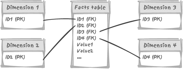
The principle of dimensional modeling is to store
measurement values, whether they are quantities, amounts, or whatever
you can imagine into big fact tables . Reference data is stored into dimension
tables that mostly contain self-explanatory labels and that
are heavily denormalized. There are typically 5 to 15 dimensions, each
with a system-generated primary key, and the fact table contains all
the foreign keys. Typically, the date associated with a series of
measures (a row) in the fact table will not be stored as a date column
in the fact table, but as a system-generated number that will
reference a row in the date_dimension table in which the date will
be declined under all possible forms. If we take,
for instance, the traditional starting date of the Unix world, January
1, 1970, it would typically be stored in date_dimension as:
| | | | | | | |
12345 | 01/01/1970 | January 1, 1970 | Thursday | January | 1970 | Q1 1970 | Holiday |
Every row that refers to something having occurred on January 1,
1970 in the fact table would simply store the 12345 key. The rationale behind such an
obviously non-normalized way of storing data is that, although
normalization is highly important in environments where data is
changed, because it is the only way to ensure data integrity, the
overhead of storing redundant information in a data warehouse is
relatively negligible since dimension tables contain very few rows
compared to the normalized fact table. For instance, a one-century
date dimension would only hold 36,525 rows. Moreover, argues Dr.
Kimball, having only a fact table surrounded by dimension tables as in
Figure 10-3 (hence the
“star schema " name) makes querying that data extremely simple.
Queries against the data tend to require very few joins, and therefore
are very fast to execute.
Anybody with a little knowledge of SQL will probably be startled by the implication that the fewer the joins, the faster a query runs. Jumping to the defense of joins is not, of course, to recommend joining indiscriminately dozens of tables, but unless you have had a traumatic early childhood experience with nested loops on big, unindexed tables, it is hard to assert seriously that joins are the reason queries are slow. The slowness comes from the way queries are written; in this light, dimensional modeling can make a lot of sense, and you’ll see why as you progress through this chapter.
Query Tools
The problem with decision-support systems is that their primary users have not the slightest idea how to write an SQL query, not even a terrible one. They therefore have to use query tools for that purpose, query tools that present them with a friendly interface and build queries for them. You saw in Chapter 8 that dynamically generating an efficient query from a fixed set of criteria is a difficult task, requiring careful thought and even more careful coding. It is easy to understand that when the query can actually be anything, a tool can only generate a decent query when complexity is low.
The following piece of code is one that I saw actually generated
by a query tool (it shows some of the columns returned by a subquery
in a from clause):
    ...
    FROM (SELECT ((((((((((((t2."FOREIGN_CURRENCY"
                             || CASE
                                  WHEN 'tfp' = 'div' THEN t2."CODDIV"
                                  WHEN 'tfp' = 'ac' THEN t2."CODACT"
                                  WHEN 'tfp' = 'gsd' THEN t2."GSD_MNE"
                                  WHEN 'tfp' = 'tfp' THEN t2."TFP_MNE"
                                  ELSE NULL
                                END
                                )
                             || CASE
                                  WHEN 'Y' = 'Y' THEN TO_CHAR (
                                          TRUNC (
                                                 t2."ACC_PCI"
                                                )
                                         )
                                  ELSE NULL
                                END
                               )
                            || CASE
                                 WHEN 'N' = 'Y' THEN t2."ACC_E2K"
                                 ELSE NULL
                               END
                              )
                           || CASE
                                WHEN 'N' = 'Y' THEN t2."ACC_EXT"
                                ELSE NULL
                               END
                              )
                           || CASE ...
It seems obvious from this sample’s select list that at least some “business
intelligence” tools invest so much intelligence on the business side
that they have nothing left for generating SQL queries. And when the
where clause ceases to be
trivial—forget about it! Declaring that it is better to avoid joins
for performance reasons is quite sensible in this context. Actually,
the nearer you are to the “text search in a file” (a.k.a. grep) model, the better. And one
understands why having a “date dimension” makes sense, because having
a date column in the fact table and expecting that the query tool will
transform references to “Q1” into “between January 1 and March 31” to
perform an index range scan requires the kind of faith you usually
lose when you stop believing in the Tooth Fairy. By explicitly laying
out all format variations that end users are likely to use, and by
indexing all of them, risks are limited. Denormalized dimensions,
simple joins, and all-round indexing increase the odds that most
queries will execute in a tolerable amount of time, which is usually
the case.
Extraction, Transformation, and Loading
In order for business users to be able to proactively leverage strategic cost-generating opportunities (if data warehousing literature is to be believed), it falls on some poor souls to ensure the mundane task of feeding the decision-support system. And even if tools are available, this feeding is rarely an easy task.
Data extraction
Data extraction is not usually handled through SQL queries. In the general case, purpose-built tools are used: either utilities or special features provided by the DBMS, or dedicated third-party products. In the unlikely event that you would want to run your own SQL queries to extract information to load into a data warehouse, you typically fall into the case of having large volumes of information, where full table scans are the safest tactic. You must do your best in such a case to operate on arrays (if your DBMS supports an array interface—that is fetching into arrays or passing multiple values as a single array), so as to limit round-trips between the DBMS kernel and the downloading program.
Transformation
Depending on your SQL skills, the source of the data,
the impact on production systems, and the degree of
transformation required, you can use the SQL language to perform a
complex select that will return
ready-to-load data, use SQL to modify the data in a staging area, or
use SQL to perform the transformation at the same time as the data
is uploaded into the data warehouse.
Transformations often include aggregates, because the granularity required by decision support systems is usually coarser than the level of detail provided by production databases. Typically, values may be aggregated by day. If transformation is not more complicated than aggregation, there is no reason for performing it as a separate operation. Writing to the database is much costlier than reading from it, and updating the staging area before updating the data warehouse proper may be adding an unwanted costly step.
Such an extra step may be unavoidable, though, when data has to be compounded from several distinct operational systems; I can list several possible reasons for having to get data from different unrelated sources:
Acute warlordism within the corporation
A recently absorbed division still using its pre-acquisition information system
A migration spread over time, meaning that at some point you have, for instance, domestic operations still running on an old information system while international ones are already using a new system that will later be used everywhere
The assemblage of data from several sources should be done, as
much as possible, in a single step, using a combination of set
operators such as union and of
in-line views—subqueries in the from clause. Multiple passes carry a
number of risks and should not be directly applied to the target
data warehouse. The several-step update of tables, with null columns being suddenly assigned
values is an excellent recipe for wreaking havoc at the physical
level. When data is stored in variable length, as is often the case
with character information and sometimes with numeric information as
well (Oracle is an example of such a storage strategy), it will
invariably lead to some of the data being relegated to overflow
pages, thus compromising the efficiency of both full scans and
indexed accesses, since indexes usually point to the head part of a
row. Any pointer to an overflow area will mean visiting more pages
than would otherwise be necessary to answer a given question, and
will be costly. If the prepared data is very simply inserted into
the target data warehouse tables, data will be properly reorganized
in the process.
It is also quite common to see several updates applied to
different columns of the same table in turn. Whenever possible,
perhaps with help from the case
construct, always update as many columns in one statement as
possible.
Loading
If you build your data warehouse (or data mart, as others prefer to say) according to the rules of dimensional modeling, all dimensions will use artificial, system-generated keys for the purpose of keeping a logical track over time of items that may be technically different but logically identical. For instance, if you manufacture consumer electronics, a new model with a new reference may have been designed to replace an older model, now discontinued. By using the same artificial key for both, you can consider them as a single logical entity for analysis.
The snag is that the primary keys in your operational database will usually have different values from the dimension identifiers used in the decision support system, which becomes an issue not with dimension tables but with fact tables. You have no reason to use surrogate keys for dates in your operational system. In the same way, the operational system doesn’t necessarily need to record which electronic device model is the successor to another. Dimension tables are, for the most part, loaded once and rarely updated. Dimensional modeling rests partly on the assumption that the fast-changing values are the ones stored in fact tables. As a result, for every row you need to insert into the fact table, you must retrieve (from the operational database primary key) the value of the corresponding surrogate, system-generated key for each of the dimensions—which necessarily means as many joins as there are different dimensions. Queries against the decision support system may require fewer joins, but loading into the decision support system will require many more joins because of the mapping between operational and dimensional keys.
Integrity constraints and indexes
When a DBMS implements referential integrity checking, it is sensible to disable that checking during data load operations. If the DBMS engine needs to check for each row that the foreign keys exist, the engine does double the amount of work, because any statement that uploads the fact table has to look for the parent surrogate key anyway. You might also significantly speed up loading by dropping most indexes and rebuilding them after the load, unless the rows loaded represent a small percentage of the size of the table that you are loading, as rebuilding indexes on very large tables can be prohibitively expensive in terms of resources and time. It would however be a potentially lethal mistake to disable all constraints, and particularly primary keys. Even if the data being loaded has been cleaned and is above all reproach, it is very easy to make a mistake and load the same data twice—much easier than trying to remove duplicates afterwards.
Querying Dimensions and Facts: Ad Hoc Reports
If query tools are seriously helped by removing anything that can get in their way, such as evil joins and sophisticated subqueries, there usually comes a day when business users require answers that a simplistic schema cannot provide. The dimensional model is then therefore duly “embellished” with mini-dimensions , outriggers , bridge tables , and all kinds of bells and whistles until it begins to resemble a clean 3NF schema, at which point query tools are beginning to suffer. One day, a high-ranking user tries something daring—and the next day the problem is on the desk of a developer, while the tool-generated query is still running. Time for ad hoc queries and shock SQL!
It is when you have to write ad hoc queries that it is time to get back to dimensional modeling and see the SQL implications . Basically, dimensions represent the breaks in a report. If an end user often wants to see sales by product, by store, and by month, then we have three dimensions involved: the date dimension that has been previously introduced, the product dimension, and the store dimension. Product and store can be denormalized to include information such as product line, brand, and category in one case, and region, surface, or whatever criterion is deemed to be relevant in the other case. Sales amounts are, obviously, facts.
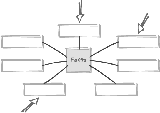
A key characteristic of the star schema is that we are supposed
to attack the fact table through the dimensions such as in Figure 10-4; in the previous
example, we might for instance want to see sales by product, store,
and month for dairy products in the stores
located in the Southwest and for the
third quarter. Contrarily to the generally
recommended practice in normalized operational databases, dimension
tables are not only denormalized, but are also strongly
indexed. Indexing all columns means that, whatever the degree of
detail required (the various columns in a location dimension, such as
city, state, region, country, area, can be seen as various levels of
detail, and the same is true of a date dimension), an end user who is
executing a query will hit an index. Remember that dimensions are
reference tables that are rarely if ever updated, and therefore there
is no frightful maintenance cost associated with heavy indexing. If
all of your criteria refer to data stored in dimension tables, and if
they are indexed so as to make any type of search fast, you should
logically hit dimension tables first and then locate the relevant
values in the fact table.
Hitting dimensions first has very strong SQL implications that we must well understand. Normally, one accesses particular rows in a table through search criteria, finds some foreign keys in those rows, and uses those foreign keys to pull information from the tables those keys reference. To take a simple example, if we want to find the phone number of the assistant in the department where Owens works, we shall query the table of employees basing our search on the “Owens” name, find the department number, and use the primary key on the table of departments to find the phone number. This is a classic, nested-loop join case.
With dimensional modeling, the picture totally changes. Instead of going from the referencing table (the employees) to the referenced table (the departments), naturally following foreign keys, we start from the reference tables—the dimensions. To go where? There is no foreign key linking a dimension to the fact table: the opposite is true. It is like looking for the names of all the employees in a department when all you know is the phone number of the assistant. When joining the fact table to the dimension, the DBMS engine will have to go through a mechanism other than the usual nested loop—perhaps something such as a hash join.
Another peculiarity of queries on dimensional models is that they often are perfect examples of the association of criteria that’s not too specific, with a relatively narrow intersection to obtain a result set that is not, usually, enormous. The optimizer can use a couple of tactics for handling such queries. For instance:
- Determining which is the most selective of all these not-very-selective criteria, joining the associated dimension to the fact table, and then checking each of the other dimensions
Such a tactic is fraught with difficulties. First of all, the way dimensions are built may give the optimizer wrong ideas about selectivity. Suppose we have a date dimension that is used as the reference for many different dates: the sales date, but also, for instance, the date on which each store was first opened, a fact that may be useful to compare how each store is doing after a given number of months of activity. Since the date dimension will never be a giant table, we may have decided to fill it from the start with seventy years’ worth of dates. Seventy years give us, on one hand, enough “historical” dates to be able to refer to even the opening of the humble store of the present chairman’s grandfather and, on the other hand, enough future dates so as to be able to forget about maintaining this dimension for quite a while. Inevitably, a reference to the sales of last year’s third quarter will make the criterion look much more selective than it really is. The problem is that if we truly had a “sales date” inside the fact table, it would be straightforward to determine the useful range of dates. If we just have a “date reference” pointing to the date dimension, the starting point for evaluation is the dimension, not the fact table.
- Scanning the fact table and discarding any row that doesn’t satisfy any of the various criteria
Since fact tables contain all the measurement or metrics, they are very large. If they are partitioned, it will necessarily be against a single dimension (two if you use subpartitioning). Any query involving three or more dimensions will require a full scan of a table that can contain millions of rows. Scanning the fact table isn’t the most attractive of options.
In such a case, visiting the fact table at an early stage, which also means after a first dimension, may be a mistake. Some products such as Oracle implement an interesting algorithm, known in Oracle’s case as the “star transformation.” We are going to look next at this transformation in some detail, including characteristics that are peculiar to Oracle, before discussing how such an algorithm may be emulated in non-Oracle environments.
Important
Dimensional modeling is built on the premise that dimensions are the entry points. Facts must be accessed last.
The star transformation
The principle behind the star transformation is, as a very first step, to separately join the fact table to each of the dimensions for which we have a filtering condition. The transformation makes it appear that we are joining several times to the fact table, but appearances are deceiving. What we really want is to get the addresses of rows from the fact table that match the condition on each dimension. Such an address, also known as a rowid (accessible as a pseudo-column with Oracle; Postgres has a functionally equivalent oid) is stored in indexes. All we need to join, therefore, are three objects:
The index on the column from the dimension table that we use as a filtering condition—for instance, the
quarterscolumn indate_dimensionThe
date_dimensionitself, in which we find the system-generated artificial primary keydate_keyThe index on the column in the fact table that is defined as a foreign key referencing
date_key(star transformations work best when the foreign keys in the fact table are indexed)
Even though the fact table appears several times in a star query, we will not hit the same data or index pages repeatedly. All the separate joins will involve different indexes, and all storing rowids referring to the same table—but otherwise those indexes are perfectly distinct objects.
As soon as we have the result of two joins, we can combine the
two resulting sets of rowids, discarding everything that doesn’t
belong to the intersection of the two sets for an and condition or retaining everything for
an or condition. This step is
further simplified if we are using bitmap
indexes , for which simple bit-wise operations are all that
is required to select our final set of rowids that refer to rows
satisfying our conditions. Once we have our final, relatively small
set of resulting rowids, then we can fetch the corresponding rows
from the fact table that we are actually visiting for the very first
time.
Bitmap indexes, as their name says, index values by keeping bitmaps telling which rows contain a particular value and which do not. Bitmap indexes are particularly appropriate to index low-cardinality columns; in other words, columns in which there are few distinct values, even if the distribution of those values is not particularly skewed. Bitmap indexes were not mentioned in previous chapters for an excellent reason: they are totally inappropriate for general database operations. There is a major reason for avoiding them in a database that incurs normal update activity: when you update a bitmap, you have to lock it. Since this type of index is designed for columns with few distinct values, you end up preventing changes to many, many rows, and you get a behavior that lies somewhere between page locking and table locking, but much closer to table locking. For read-only databases, however, bitmap indexes may prove useful. Bitmap indexes are quickly built during bulk loads and take much less storage than regular indexes.
Emulating the star transformation
Although automated star transformation is a feature that enables even poorly generated queries to perform efficiently, it is quite possible to write a query in a way that will induce the DBMS kernel to execute it in a similar, if not exactly identical, fashion. I must plead guilty to writing SQL statements that are geared at one particular result. From a relational point of view, I would deserve to be hanged high. On the other hand, dimensional modeling has nothing to do with the relational theory. I am therefore using SQL in a shamelessly unrelational way.
Let’s suppose that we have a number of dimension tables named
dim1, dim2, ...dim n. These
dimension tables surround our fact table that we shall imaginatively
call facts. Each row in facts is composed of key1, key2, ...key n, foreign
keys respectively pointing to one dimension table, plus a number of
values (the facts) val1, val2, ...val p. The
primary key of facts is defined
as a composite key, and is simply made of key1 to key n.
Let’s further imagine that we need to execute a query that
satisfies conditions on some columns from dim1, dim2, and dim3 (they may, for instance, represent a
class of products, a store location, and a time period). For
simplicity, say that we have a series of and conditions, involving col1 in dim1, col2 in dim2 and col3 in dim3. We shall ignore any transformation,
aggregate or whatever, and limit our creative exercise to returning
the appropriate set of rows in as effective a way as
possible.
The star transformation mostly aims to obtain in an efficient
way the identifiers of the rows from the fact table that will belong
to our result set, which may be the final result set or an
intermediate result set vowed to further ordeals. If we start with
joining dim2 to facts, for instance:
    select ...
    from dim2,
         facts
    where dim2.key2 = facts.key2
      and dim2.col2 = some value
then we have a major issue if we have no Oracle
rowid, because the identifiers of the
appropriate rows from facts are
precisely what we want to see returned. Must we return the primary
key from facts to properly
identify the rows? If we do, we hit not only the index on facts(key2), but also table facts itself, which defeats our initial
purpose. Remember that the frequently used technique to avoid an
additional visit to the table is to store the information we need in
the index by adding to the index the columns we want to return. So,
must we turn our index on facts(key2) into an index on facts(key2, key3...keyn)? If we do that, then we must apply
the same recipe to all foreign keys! We will end up with
n indexes that will each be of a size in the
same order of magnitude as the facts table itself, something that is not
acceptable and that forces us to read large amounts of data while
scanning those indexes, thus jeopardizing performance.
What we need for our facts
table is a relatively small row identifier—a surrogate key that we
may call fact_id. Although our
facts table has a perfectly good
primary key, and although it is not referenced by any other table,
we still need a compact technical identifier—not to use in other
tables, but to use in indexes.
With our system-generated fact_id column, we can have indexes on
(key1, fact_id), (key2, fact_id)...(keyn, fact_id) instead of on the foreign
keys alone. We can now fully write our previous query as:
selectfacts.fact_idfrom dim2, facts where dim2.key2 = facts.key2 and dim2.col2 =some value
This version of the query no longer needs the DBMS engine to
visit anything but the index on col2, the dimension table dim2, and the facts index on (key2, fact_id). Note that by applying the
same trick to dim2 (and of course
the other dimension tables), systematically appending the key to
indexes on every column, the query can be executed by only visiting
indexes.
Repeating the query for dim1 and dim3 provides us with identifiers of facts
that satisfy the conditions associated with these dimensions. The
final set of identifiers satisfying all conditions can easily be
obtained by joining all the queries:
    select facts1.fact_id
    from (select facts.fact_id
          from dim1,
               facts
          where dim1.key1 = facts.key1
            and dim1.col1 = some value) facts1,
          (select facts.fact_id
           from dim2,
                facts
           where dim2.key2 = facts.key2
             and dim2.col2 = some other value) facts2,
           (select facts.fact_id
            from dim3,
                 facts
            where dim3.key3 = facts.key3
              and dim3.col3 = still another value) facts3
    where facts1.fact_id = facts2.fact_id
       and facts2.fact_id = facts3.fact_id
Afterwards, we only have to collect from facts the rows, the identifiers of which
are returned by the previous query.
The technique just described is, of course, not specific to decision-support systems. But I must point out that we have assumed some very heavy indexing, a standard fixture of data marts and, generally speaking, read-only databases. In such a context, putting more information into indexes and adding a surrogate key column can be considered as “no impact” changes. You should be most reluctant in normal (including in the relational sense!) circumstances to modify a schema so significantly to accommodate queries. But if most of the required elements are already in place, as in a data warehousing environment, you can certainly take advantage of them.
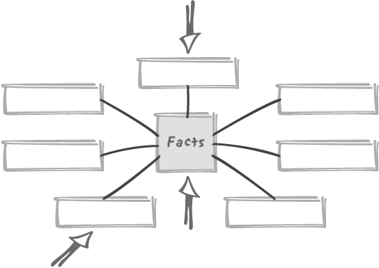
Querying a star schema the way it is not intended to be queried
As you have seen, the dimensional model is designed to be queried through dimensions. But what happens when, as in Figure 10-5, our input criteria refer to some facts (for instance, that the sales amount is greater than a given value) as well as to dimensions?
We can compare such a case to the use of a group by. If the condition on the fact
table applies to an aggregate (typically a sum or average), we are
in the same situation as with a having clause: we cannot provide a result
before processing all the data, and the condition on the fact table
is nothing more than an additional step over what we might call
regular dimensional model processing. The situation
looks different, but it isn’t.
If, on the contrary, the condition applies to individual rows
from the fact table, we should consider whether it would be more
efficient to discard unwanted facts rows earlier in the process, in
the same way that it is advisable to filter out unwanted rows in the
where clause of a query, before
the group by, rather than in the
having clause that is evaluated
after the group by. In such a
case, we should carefully study how to proceed. Unless the fact
column that is subjected to a condition is indexed—a condition that
is both unlikely and unadvisable—our entry point will still be
through one of the dimensions. The choice of the proper dimension to
use depends on several factors; selectivity is one of them, but not
necessarily the most important one. Remember the clustering factor
of indexes, and how much an index that corresponds to the actual,
physical order of rows in the table outperforms other indexes
(whether the correspondence is just a happy accident of the data
input process, or whether the index has been defined as constraining
the storage of rows in the table). The same phenomenon happens
between the fact table and the dimensions. The order of fact rows
may happen to match a particular date, simply because new fact rows
are appended on a daily basis, and therefore those rows have a
strong affinity to the date dimension. Or the order of rows may be
strongly correlated to the “location dimension” because data is
provided by numerous sites and processed and loaded on a
site-by-site basis. The star schema may look symmetrical, just as
the relational model knows nothing of order. But implementation
hazards and operational processes often result in a break-up of the
star schema’s theoretical symmetry. It’s important to be able to
take advantage of this hidden dissymmetry whenever possible.
If there is a particular affinity between one of the dimensions to which a search filter must be applied and to the fact table, the best way to proceed is probably to join that dimension to the fact table, especially if the criterion that is applied to the fact table is reasonably selective. Note that in this particular case we must join to the actual fact table, obviously through the foreign key index, but not limit our access to the index. This will allow us to directly get a superset of our target collection of rows from the fact table at a minimum cost in terms of visited pages, and check the condition that directly applies to fact rows early. The other criteria will come later.
A (Strong) Word of Caution
Dimensional modeling is a technique, not a theory, and it is popular because it is well-suited to the less-than-perfect (from an SQL[*] perspective) tools that are commonly used in decision support systems, and because the carpet-indexing (as in “carpet-bombing”) it requires is tolerable in a read-only system—read-only after the loading phase, that is. The problem is that when you have 10 to 15 dimensions, then you have 10 to 15 foreign keys in your fact table, and you must index all those keys if you want queries to perform tolerably well. You have seen that dimensions are mostly static and not enormous, so indexing all columns in all dimensions is no real issue. But indexing all columns may be much more worrisome with a fact table, which can grow very big: just imagine a large chain of grocery stores recording one fact each time they sell one article. New rows have to be inserted into the fact table very regularly. You saw in Chapter 3 that indexes are extremely costly when inserting; 15 indexes, then, will very significantly slow down loading. A common technique to load faster is to drop indexes and then recreate them (if possible in parallel) once the data is loaded. That technique may work for a while, but re-indexing will inexorably take more time as the base table grows. Indexing requires sorting, and (as you might remember from the beginning of this chapter) sorts belong to the category of operations that significantly suffer when the number of rows increases. Sooner or later, you will discover that the re-creation of indexes takes way too much time, and you may well also be told that you have users who live far, far away who would like to access the data warehouse in the middle of the night.
Users that want the database to be accessible during a part of the night mean a smaller maintenance window for loading the decision support system. Meanwhile, because recreating indexes takes longer as data accumulates into the decision support database, loading times have a tendency to increase. Instead of loading once every night, wouldn’t it be possible to have a continuous flow of data from operational systems to the data warehouse? But then, denormalization can become an issue, because the closer we get to a continuous flow, the closer we are to a transactional model, with all the integrity issues that only proper normalization can protect against. Compromising on normalization is acceptable in a carefully controlled environment, an ivory tower. When the headquarters are too close to the battlefield, they are submitted to the same rules.