CHAPTER |
|
13 |
SQL Spatial: Backend Databases for Spatial Data |
We’re at a point now to discuss the storage of large volumes of spatial data in databases. What good is it to annotate maps with markers and shapes if you can’t store these features into a central database and reuse it as needed? While KML will serve you well for isolated features and small-scale applications, as you accumulate more and more data the need for central storage will become pressing. The question of storing large sets of data isn’t unique to spatial data; it’s a universal problem and it’s addressed with databases.
Database Management Systems (DBMS) are special systems designed for storing large volumes of data. You can also use very large files to store data, but databases are very complex objects that abstract the complexity of manipulating individual data items and provide mechanisms to quickly locate the items you’re interested in. Traditionally, DBMSs were designed to handle typical business and scientific data types, such as text, numbers, and dates. Modern databases, such as SQL Server and Oracle, can also handle spatial data.
Do You Really Need Spatial Databases?
You can store the numeric values that represent longitude/latitude pairs as numeric values in any database table, can’t you? That’s true, but when it comes to querying the data, you’d have to write some serious code to efficiently locate the items you’re interested in. Such items could be all hotels within a 5-mile radius from your current location, or the cities that fall into a polygon that represents a county. Thanks to Google, you don’t have to write any code to perform distance calculations in your scripts. If your data resides in a database, however, you should be able to perform similar queries with ease. And this is exactly why a new data type is needed. All major DBMSs include support for spatial queries, which enables you to quickly retrieve data based on geographical features. You will find many examples of querying data with a spatial component in this chapter, but let’s start by examining how spatial data are stored in databases and how spatial data are described.
Using Tables with Spatial Features
While all major DBMSs (such as SQL Server, Oracle, MySql, and so on) support spatial data, this chapter deals with SQL Server’s spatial features. I selected SQL Server because there’s a free version, SQL Server 2012 Express, which fully supports spatial features. As for the methods you use to query spatial data, they’re part of the OGC (Open GeoSpatial Consortium) standard and are supported by both Oracle and MySql. The topic of handling spatial data is huge, and this chapter is only an introduction to the spatial features supported by SQL. In this chapter, you learn about the methods you’ll use to retrieve spatial data from a SQL server in the context of developing map-enabled applications with the Google Maps API.
All major databases provide a language for manipulating the data, and all languages are based on the SQL standard (Structured Query Language). The examples in this chapter are written in T-SQL (Transactional SQL), which is the language of SQL Server. T-SQL is based on SQL and it contains its own extensions to standard SQL. Oracle’s SQL is called PL/SQL (Procedural Language/SQL); it supports the core of SQL and enhances it with its own extensions. All queries in this chapter are standard SQL queries and use the OGC geography extensions.
To start your exploration of spatial data, you can open the
Samples.sql file, which comes with this book’s support material in SQL Server’s Management Studio, and execute it. It will create a new database, the GEO database, and will add five tables:• USCities Contains city names along with populations and geo-locations.
• USStates Contains just state names and is used in conjunction with the USCities table.
• World Airports Contains the names and locations for 9,000 airports around the world. Use the data in the World Airports table to execute spatial queries on non-trivial data.
• Highways Contains the paths of two major highways, the US 5 and US 101.
• CountyBorders Contains the outlines of a few counties in California.
One of the table names contains a space, and this table’s name must be embedded in square brackets in the corresponding queries. The brackets are not used in the text, just in the queries involving this table. The last two tables will be used later in the chapter with examples that involve lines and polygons. In the course of this chapter, you will see how these tables were populated and how to insert additional data, if you’re interested.
To populate the tables, execute the remaining SQL scripts in this chapter’s support material. The scripts are presented in the sidebar “The SQL Scripts to Populate the Sample Tables” later in this chapter.
The examples will also work with SQL Server 2008 (including the 2008 Express version) with one exception: The
STContains method was introduced with SQL Server 2012 and was not supported by earlier versions. If you don’t need to select points that lie within specific polygons, all supported versions of SQL Server will do. This method, however, is too convenient to ignore and you should consider switching to version 2012 of SQL Server.This chapter contains no JavaScript code, or applications. It’s an introduction to the topic of handling geospatial data with SQL Server, and all examples are queries that can be executed in SQL Server Management Studio.
Designing the Sample Tables
Let’s start with a quick overview of the tables you’re going to see in the examples. The
Samples.sql script will create the GEO database for you and it will add the tables mentioned. Assuming that you have installed one of the versions of SQL Server 2008 or 2012 on your computer, double-click the Samples.sql file and it will open in SQL Server’s Management Studio in a new Query window. Execute the script, and the database will be set up for you. Then, switch to the GEO database and explore its tables and their structure.You can also create the tables on your own with the table editor in SQL Server’s Management Studio. Just right-click the Tables item under the GEO database and you’ll be presented with a nice interface that allows you to specify column names and types. If you want to see, and possibly edit, the tables created by the script, right-click a table name in the left pane of Figure 13-1 and select the Design command. The World Airports table, for example, contains the columns shown in the following table.
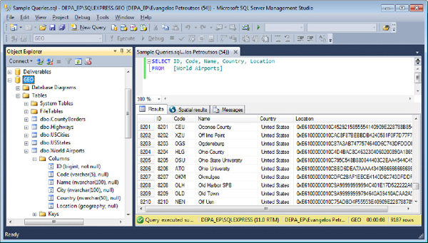
Figure 13-1 The results of a query that selects all the rows from the [World Airports] table in the Results pane
| Column Name | Data Type |
| ID | bigint |
| Code | varchar(5) |
| Name | varchar(100) |
| City | varchar(50) |
| Country | varchar(50) |
| Location | geography |
The ID column is an Identity column (it’s assigned a unique value every time a new row is added). The remaining columns store text, except for the last one, which stores spatial data. The Location column is of the
geography type and stores geography features of any type: points, lines, and polygons.The Location column of the World Airports table stores points only because all airports are identified by a pair of latitude/longitude values. You usually don’t mix features with different geometries in the same column. In other words, you avoid storing points and polygons in the same column because this will complicate your queries. If a column contains both points and polygons, it wouldn’t make much sense to request the area or the length of the points. You would have to keep track of each item’s
geography type so it’s best to store different geography types in different columns, or different tables. By the way, SQL Server won’t crash if you attempt to calculate the length or the area of a point; it will simply return the value null.Figure 13-1 shows the results of a query that selects all rows in the World Airports table and displays them as text in the Results pane. The Location column is a binary column, and you will see later in this chapter how to display locations in a human-readable format.
Figure 13-2 shows the distribution of the airports on the latitude/longitude grid, shown in the Spatial Results pane. This grid is basically a map without a background; SQL Server Management Studio populates this grid automatically with points, lines, and polygons, depending on the query.

Figure 13-2 Viewing the airports as points on the Spatial Results pane of SQL Server’s Management Studio
The remaining sample tables have a similar structure: an ID value that identifies each row, a number of text columns, and a
geography column to store the geospatial data. In the World Airports table, the Location column stores the location of the corresponding airport. In the Highways table, the geography column is called Route and it stores a path (the highway’s route). This table contains two highways: US 5 and, US 101 and is shown in the following table. The Route column of this table stores a LineString object, which is equivalent to the Polyline object of the Google Maps API. The CountyBorders table stores the polygons that outline each county; in the Border column.| Column Name | Data Type |
| ID | bigint |
| Highway | varchar(20) |
| Route | geography |
Inserting Spatial Data
The first really non-trivial task is to insert geospatial data in your tables. Inserting data into the text columns is straightforward, but how about the geography data? There are several ways to represent geography data and they’re explained in the following sections. After you understand how to insert geographical data into a table, you’ll see how to perform elaborate queries based on geographical data.
There are three ways to represent spatial data: the Well-Known Text format, the Well-Known Binary format, and the GML (Geography Markup Language) format. All three formats are discussed in the following sections.
Well-Known Text Representation of Geography Data
There are three types of well-known strings to represent the three basic geographical features (points, lines, and polygons), and they have the same form: They start with the name of the entity followed by one or more points in parentheses. Point entities are followed by a single location, while lines and polygons are followed by a series of locations.
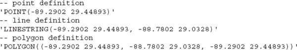
The coordinates are specified just as with KML files: Longitude and latitude values are separated by spaces, and consecutive points are separated by commas. Lines and polygons are usually followed by a large number of points; the samples here show a line and a polygon with very few vertices. Note that polygon coordinates are embedded in two pairs of parentheses, and you will see why in the following sidebar.
To convert the well-known text representation of the various items into geography data suitable for use by the
INSERT statement, pass them as arguments to the methods STPointFromText(), STLineFromText(), and STPolyFromText() of the geography data type. The following expressions are valid values for geography data, and they can be used in an INSERT statement to populate a geography column: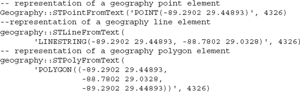
All three methods accept a second argument, which is a numeric value that identifies the so-called SRID: the Spatial Reference System Identifier. This value identifies the projection system in use. The value 4326 identifies the Mercator projection, so if you need a database of geography features to use with Google Maps, just memorize the value 4326 as the SRID of your data.
There are many reference systems in use today, and all major GIS vendors, as well as authorities such as the European Petroleum Survey Group, have their own reference system or have adopted one of them. It’s also possible to convert between different reference systems, and you can even store entities in the same table with different SRIDs. Keep in mind, however, that you can’t perform any spatial operations with data from different reference systems.
Polygons may contain holes, which are also polygons, and so the proper syntax to specify polygons involves arrays of polygons. This well-known text notation is made up of multiple arrays of points:
Note that the polygon is made up of one or more exterior rings and one or more interior rings. Even if a polygon has no holes, the coordinates of its vertices must still be enclosed in two pairs of parentheses. To insert a polygon in a
geography column, use an expression like the following:
There’s a shorter method, too, namely to skip the call to the
STPolyFromText() method. The following statement inserts a new row to the CountyBorders table: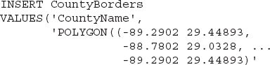
The short method of defining geography features assumes that all features are specified in the 4326 SRID, which is the proper setting for Mercator projections. If you need to specify a different SRID, you must use the
STPolyFromText() method.Polygons with Holes
In Chapter 8, you saw how to create polygons with holes on top of Google Maps. You used the following JavaScript statements to create the outline of the state of Utah and the Utah Lake as a hole in the state’s polygon (the ellipses indicate missing vertices).

The same coordinates can be used to create a POLYGON structure in SQL. The polygon is made up of two segments, one that corresponds to the state of Utah and another nested one that corresponds to the Utah Lake. Here’s a SQL statement that creates two nested POLYGON structures and then displays them. The statement doesn’t store the shape in any database; it simply assigns the definition of the shape to a variable and then selects this variable.
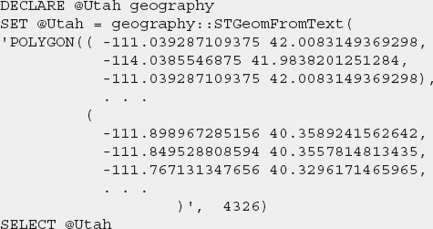
Figure 13-3 shows the query and the Spatial Results pane of the SQL Server Management Studio, where you can see the outer polygon with the outline of the state and inner polygon rendered as a hole with the shape of the lake. The script shown in the figure is
Utah Polygon.sql.
Figure 13-3 A polygon with nested paths. The nested paths (only one is shown in this example) are rendered as holes in the outer polygon.
Point features are inserted a very similar statement, which is much shorter because it contains the coordinates of a single point:
Well-Known Binary Representation of Geography Data
In addition to the well-known text format for specifying geography features, you can use the well-known binary format as well. The various features (points, lines, and polygons) are stored by SQL Server in binary format and this format is well documented by Microsoft. You will not use the binary format in this chapter, but a typical application of this format is to extract data in binary format from one table and insert the same data into another table.
The binary value of a feature is the long string you see in Results pane of SQL Server Management Studio, and it’s totally meaningless to humans. You can still store these binary values in variables and use them later as needed.
GML Representation of Geography Data
The last format is GML, which stands for Geography Markup Language. GML is an XML variation for describing geography features, similar to KML. GML is quite verbose and you will use it only to extract data from a database and move it to another one, or another system capable of understanding GML.
To retrieve the outlines of the various California counties in GML format, apply the
AsGml() method to the Border column:The result is a list of county names and links to GML segments that describe the outline of each county, as shown in Figure 13-4.

Figure 13-4 Retrieving county outlines in GML notation
If you click one of the links, you will see the GML description of the selected county’s outline. This description is something like:
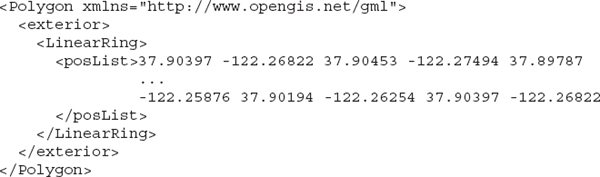
The outlines contain too many points to list here and the ellipses indicate points that have been skipped. The GML format looks very similar to KML. After all, both formats describe geography features and they’re both based on XML. The
LinearRing element is the same as in KML, but you must replace the <posList> tag under it with the <coordinates> tag. Creating the GML description of a feature is certainly the least efficient method to insert data into a geography column, but it may come in handy if you already have a collection of geospatial features in GML format. Another detail to keep in mind is that GML uses the space to delimit individual coordinates as well as consecutive points. There are no commas between consecutive points in a <posList> element in GML.Outer and Inner Polygons
Polygons must be specified in a clockwise fashion. A polygon drawn in counterclockwise fashion is a hole. If such a polygon lies within another, then it represents a hole in the outer polygon. On its own, however, it still represents a hole! It’s a hole in another polygon that spans the entire globe.
To understand how this works, let’s create a polygon that outlines the state of California. If the points are specified in a clockwise fashion, then they will generate a polygon with the shape of California, and this is the “desired” interpretation of the points that make up the polygon. If the points are specified in the opposite direction, they will generate a polygon that spans the entire globe, except for the state of California. Figure 13-5 shows two polygons with the vertices that delimit the state of California.
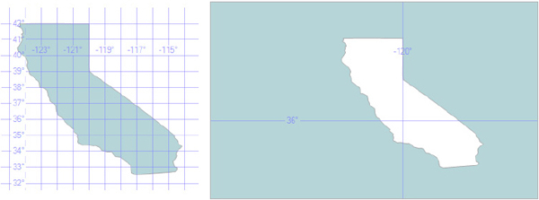
Figure 13-5 The outline of California defined in both directions. When the outline’s vertices are specified in the wrong direction, the resulting polygon covers the entire globe and the intended shape becomes a hole.
The small filled polygon that resembles the state of California was created with a POLYGON structure that contains the vertices that make up California’s outline in the correct order: in a clockwise direction. The other filled polygon was created with the same POLYGON structure, only this time the coordinates of California’s vertices were reversed. This polygon represents a hole the size and shape of California. A hole into what? Because the shape doesn’t belong to another one, it will become a hole on the entire globe. The two polygons that represent the state of California are stored in the StateOutlines table and were inserted with two simple statements.
Some simple calculations with two shapes will verify these claims. First, let’s calculate the total area of California with the
STArea() method. This method is discussed later in the chapter, but here’s the statement that uses SQL Server’s spatial methods to calculate the area of a polygon:This statement returned the numeric value 419,366,861,058.543. This is nearly half a million square kilometers. To calculate the area of the other shape that spans the entire globe, apply the same method to the row whose
ID is 2. The result is 509,646,254,849,938, which is half a billion square miles. The sum of the two should be earth’s total area:The
SUM() function returns the numeric sum of the column specified as an argument and for the two polygons it returned the value 510,065,621,710,996, or 510,065,621 square kilometers. This value is pretty close to earth’s total area as reported by Wikipedia (510,072,000 square kilometers). The difference is less than 1 part in 10,000.You can also calculate the earth’s total area, considering it’s a perfect sphere with a radius of 6,371 kilometers. The area of a sphere’s surface is given by the following calculation:

The result is 510,064,471.90, which is even closer to the value returned by the
STArea() function. As mentioned in Chapter 1, Google Maps approximate the earth with a perfect sphere, which is not quite accurate. The total area of the earth has no practical meaning because the earth’s surface is not smooth. Approximating the earth by a sphere introduces just a marginal error, but the mountains on the surface of the earth can make an enormous difference when you calculate the earth’s area.To experiment with the two polygons of California, use the StateOutlines sample table, which contains two rows with the IDs 1 (the state of California) and 2 (the reversed shape). The two outlines are identical, except for the order of their vertices. Execute the
CaliforniaOutlines.sql file to create the table and populate it with the two shapes of California.Handling Spatial Data with SQL Server Management Studio
Spatial data can be points, lines, and polygons, or collections of these types. SQL Server supports two types of spatial data: geometry and geography data. The difference is that geography data is expressed in terms of latitude and longitude (and optionally altitude) coordinates, while geometry data is arbitrary (any coordinate system will do). The examples in this chapter deal exclusively with spatial data of the
geography type.Just as you create columns of the appropriate type to store simple data (text, numbers, and dates), you can create a column of the
geography type and store geospatial data in it. It doesn’t matter what type of geography feature you store in this column. SQL Server will recognize points, lines, and polygons in a column of this type. Of course, you usually set up different columns for different entity types.Figure 13-1 shows the SQL Server Management Studio with some this chapter’s sample data. On the left pane is the structure of the World Airports table, and on the right pane is a query that selects all airports and the results of the query. The table contains data for over 9,000 airports all over the world. The data was obtained from www.openflights.org, a site that provides this information for free but will accept your donation. They also maintain a database with airlines and another one with flight routes.
The SQL Scripts to Populate the Sample Tables
The
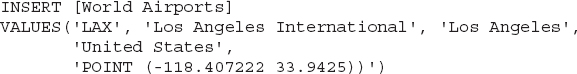
Insert Airports.sql script inserts the airport data in the World Airports table and contains a series of INSERT statements like the following:
The
Insert State Cities.sql script, which inserts the cities in the USCities table (and the states in the USStates table), is also a series of INSERT statements, only this time the statements are slightly more complex: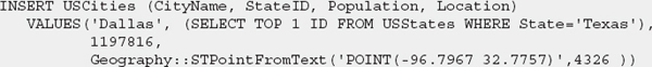
The list of values contains a subquery, which retrieves the ID of the corresponding state, but this is not related to geospatial data. The city coordinates are specified with the
STPointFromText() method, which accepts as an argument a POINT feature.The county borders are inserted into the CountyBorders table as
POLYGON features with the Insert Counties.sql script, which contains statements like the following: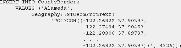
The last script,
Insert Highways.sql, contains two statements that insert two very long paths to the Highways table, one for each of the US 5 and US 101 highways:
In Figure 13-1, you saw the result of the following query:
The airport locations are spatial data (points, to be exact) and are displayed as text-encoded binary data. Regardless of the techniques for inserting spatial data into a SQL Server table, SQL Server stores the spatial data internally in a binary format.
If you want to see the actual coordinates, change the query to apply the
STAsText() method to the Location column:This time, the query returns the coordinates of each airport in a format suitable for humans, as you can see in the table that follows.
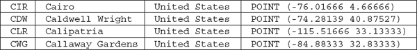
This is the well-known text format, which is suitable for humans. The actual data are maintained by SQL Server as binary values, which are converted by the
STAsText() method into text format.CAUTION While all keywords in T-SQL are case-insensitive, the names of the spatial methods, which are extensions to T-SQL, are case-sensitive. You can actually mix and match case-sensitive with case-insensitive keywords in the same statement, which is a rather odd behavior. T-SQL has always been case-insensitive, but the spatial extensions are case-sensitive.
Viewing Spatial Data on the Map
If the result set contains a spatial column, a new tab is added to the pane with the results, the Spatial Results pane, which is shown in Figure 13-2. The revised query that makes use of the
STAsText() method doesn’t contain any spatial data because the locations of the airports were retrieved as strings. Remove the STAsText() method from the Location column and execute the following query to see the Spatial Results pane:The spatial data are displayed as strings; this format is totally unsuitable for humans, but you can actually see the data points on a grid in the second tab. Switch to the Spatial Results pane to view the locations of the airports. Airport locations are shown as dots on the map. There’s no map, of course, just a grid with the coordinates. The density of the airports, however, is such that their locations practically outline all continents. Even though the Spatial Results tab doesn’t display more than 5,000 points, that’s a lot. Note that you can specify the projection used to display the results in the “Selected projection” combo box. Settings include EquiRectangular, Mercator, Robinson, and Bonne.
OGC vs. Extended Geography Methods
You can request that spatial columns be returned as readable text or as GML, with the methods
STAsText() and AsGml(), respectively. You may have noticed an inconsistency in the naming scheme of these methods (and a few others you will read about later). All methods that belong to the OGC (Open Geography Consortium) specification begin with the ST prefix. The other methods are extended methods of the geography data type and are unique to SQL Server. The STAsText() method is an OGC method, while AsGml() is an extension to T-SQL.Querying Spatial Data
The main function of a database is not the storage of data. Databases are designed to facilitate the selection of the data. The operations for inserting and deleting data are not as efficient as they could be because the database has to maintain additional information that assists the fast retrieval of data. Without the spatial data types, you’d have to write some serious code to query your data. For example, how easy would it be to find out if two polygons intersect, or even select the cities (points) that lie in a specific state (polygon)? Querying such a database would be nearly impossible without advanced calculus.
The
geography data type allows developers to write code to perform similar queries very easily. This is the reason why spatial data are represented with their own data type and this is why databases provide special methods for handling spatial data. As you will see shortly, you can write a simple query that allows you to select the airports within a specific range from a location, cities that lie within a specific state or country, and so on. The function STDistance(), for example, returns the distance between two points in meters, which means that you don’t have to supply your own code to calculate distances. The spatial features of SQL allow you to query tables based on geography data very efficiently. In this section, you’ll read about the basic spatial functions of SQL and how they’re used in queries.All the methods you’re going to explore in this and the following sections are extensions to the
geography type: They apply to a variable or column of the geography type and they accept as arguments another geography instance. In other words, there’s no function that calculates the distance between two points; you can’t write the following in T-SQL:where
@p1 and @p2 are two properly declared and initialized variables that represent points. Instead, there’s an STDistance() method, which can be applied to either one of the variables and accepts the other variable as an argument:The
STDistance() method will return the distance between the points @p1 and @p2. If you reverse the role of the two variables, the method will still return the same result:Calculating Distances
You have seen the syntax of the
STDistance() method in the introduction to this section; let’s exercise it by calculating the distance between two airports, the LAX and JFK airports: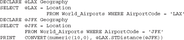
The distance between the two airports is 3,982,550 meters, or 3,892 kilometers. This is the length of the geodesic path between the two airports and it’s the same distance returned by the
calculateLength() method of the Google Maps API. Let’s write a query that calculates the distances of all U.S. airports from the Lambert–St. Louis International airport. Start by declaring a geography variable that corresponds to the location of the airport:Now write a
SELECT statement using the STDistance() method to calculate the distances of all other airports from the St. Louis International airport:The
WHERE clause was added to exclude from the result the St. Louis airport. It’s not required, but there’s no reason to include a pair of airports in the result that are 0 meters apart from one another.The result of the preceding query is a list of airport codes and names, and their distance from the St. Louis International Airport, as you can see in the table that follows.

You can modify the query a little so that it selects all airports that are within a circle of 200 kilometers from the St. Louis airport, or any other location. This time, the
STDistance() function must also be included in the WHERE clause to limit the number of qualifying airports. Listing 13-1 shows the revised query.Listing 13-1 Selecting airports within range from the World Airports table

The result of the query is shown in Figure 13-6. This query doesn’t return any spatial data because it does not include the Location column. To see the distribution of the airports on the map, you should include the Location column as the last item in the selection list.

Figure 13-6 Viewing all U.S. airports within 200 kilometers from the St. Louis International Airport and their distance from this airport
Line Lengths and Polygon Areas
You have seen the
calculateLength() and calculateArea() functions of the Google API in Chapter 10. These two methods calculate the length of a line (or path, in terms of the Google API) and the area of a polygon. SQL Server provides the STLength() and STArea() methods, which perform the same calculations. The functions of SQL Server are extremely fast, however, because SQL statements are executed on a powerful server and not at the client. As efficient as JavaScript may be, it’s an interpreted language that can’t beat a highly optimized and extremely specialized language like T-SQL. Moreover, T-SQL can use the STLength() method to quickly calculate the lengths of hundreds or thousands of lines and return the one with the longest or shortest length and even order a large number of lines according to their lengths.The CountyBorders table contains California’s counties with columns for their names (column
Country) and their geography (column Border). To calculate the perimeter of a country, apply the STLength() method to the Border column. Likewise, to calculate the area of a county, apply the STArea() method to the same column. The following statement returns the names, perimeters, and areas of all counties in the CountyBorders table: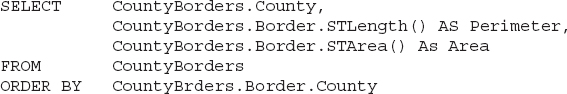
Note that you need not prefix the column names by their table name, because the query involves a single table.
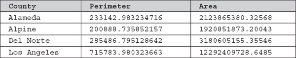
The output of this statement (the first few counties) is shown in the following table.
To change the order of the results, specify one of the other two expressions in the selection list after the
ORDER BY clause. To retrieve the largest county, use the following expression, which calculates the area of all counties, sorts them in descending order, and returns the top row only: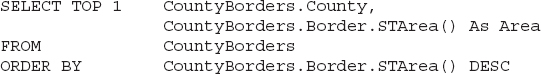
The largest county is Riverside with an area of 18,892,717,528.5141 square meters, or 18,892.72 square kilometers. According to Wikipedia, the area of Riverside is 18,915 square kilometers; the more points you add along the perimeter of the county, the more closely you will approximate the county. Even with a fairly rough outline, the error is 80 units in 19,000 units, which is less than 0.5 percent.
The
STDistance() method accepts as an argument a geography instance, which isn’t necessarily a point. You can use this method to calculate the distance between two points, or the distance between a point and a polygon, or even the distance between two polygons. For the latter, the distance is the length of the shortest possible line that can be drawn between the two polygons.Let’s apply the
STDistance() method to calculate the distance from all counties to the LAX airport in Santa Monica. Listing 13-2 shows the query.Listing 13-2 Calculating distances of counties from the LAX airport
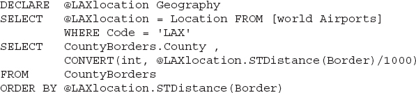
Note that the location of LAX is not hard-coded. Instead, it’s retrieved from the World Airports table. The rest of the query deals with the CountyBorders table: It passes the geography of each state, the
Border column, to the STDistance() method as an argument to calculate the distances, and then it orders the results based on this distance.
LAX airport lies within Los Angeles County, and its distance from Los Angeles County is zero. Any point that lies within a polygon has a distance of 0 from the same polygon.
You can also create a stored procedure to retrieve the airports that lie within a specific range from any given location. The location and the maximum distance are arguments of the stored procedure. The
SelectAirportsInRange() stored procedure does exactly that, as you can see in Listing 13-3.Listing 13-3 The definition of the
Select Airports InRange() stored procedure
The
rangeInKM argument is the maximum distance expressed in kilometers. To execute this procedure, set up a geography variable with the desired location and a maximum distance: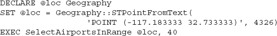
This query will return a list of airports like the one shown in Figure 13-7.

Figure 13-7 Executing a stored procedure against the World Airports table
Intersections
Another very useful set of methods in SQL spatial extensions deals with shape intersections. Note that there are no equivalent methods in the Google API. The
STIntersects() method detects whether two geographies intersect or not and returns a true/false value, while the STIntersection() method returns the geography of the intersection. If you use the STIntersection() method with a line and a polygon, for example, the method will return a line, which is the segment (or segments) of the line that lies within the polygon. If you use it with two lines, the same method will return the point where the two lines meet. To interpret correctly the result of the STIntersects() method, you need to know the type of the intersecting geographies.Let’s find the part of US 101 that lies within Los Angeles County. This is a typical operation that can’t be performed with the methods of the Google Maps API. On the other hand, it’s practically trivial with SQL Server’s spatial methods. The route of US 101 is represented in the Highways table with a
LINESTRING primitive that contains 1,745 vertices. The locations of these vertices were obtained by tracing the freeway on the map with the Map Traces sample project of Chapter 9. To view the path of US 101 limits, execute the following query against the Highways table in the GEO database.In Figure 13-8, you see that only a segment of US 101 was traced, but it’s a fairly lengthy segment starting in Los Angeles and extending all the way to San Francisco (695.584 kilometers in all).

Figure 13-8 The route of US 101 on the Spatial Results tab of SQL Server Management Studio
Create two
geography instances to store the polygon that outlines Los Angeles County and the line that corresponds to the highway. The following are the two statements that retrieve the desired data from the corresponding tables:
Now you’re ready to calculate the intersection of the two instances, which is the part of the freeway that lies in Los Angeles County. The method
STIntersects() lets you know if the two geographies intersect at all:
The
STIntersection() method goes one step further: It returns the intersection of the instance defined by its argument with the instance to which the method is applied. Replace the IF statement of the preceding example with a call to the STIntersection() method of the @geo_shape variable:Figure 13-9 shows the result of the query in the Spatial Results pane. What you see is the segment of the line that lies within the specified polygon and it’s the part of US 101 in Los Angeles County. If you commute on this highway daily, you’ll probably recognize it.

Figure 13-9 The segment of US 101 highway in Los Angeles County
To actually get the definition of the segment of US 101 within Los Angeles County, apply the
STAsText() method to the result:This time, the result is a textual description of the same line, and it will appear in the Result pane of the SQL Management Studio as a
LINESTRING primitive: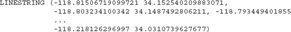
If you need to know the coordinates of the points of the intersection, request the starting and ending points of the intersection with the
STStartPoint() and STEndPoint() methods. Just replace the SELECT statement in the preceding example with the following statements that create the @line variable to hold the intersection geometry, and then apply the two methods to retrieve the endpoints of this variable:
The preceding statements will generate the following output:
Copy the coordinates of the points returned by the query and locate these points on the map. You must also reverse the order of latitude and longitude values when you paste them into Google Maps. To locate the first intersection point, enter the string
34.152540209883071, -118.81506719099721 in the search box of Google Maps. The two endpoints correspond to Thousand Oaks and downtown Los Angeles.Using Intersections as Selection Criteria
The preceding example was rather simplistic because it requested a single intersection of two specific geography instances. A much more useful type of query is one that retrieves the segments of the highway that fall within each county. This time, let’s apply the
STIntersection() method to each county’s border in the CountyBorders table, passing as an argument the definition of the line that represents the freeway:
The query returns the intersection of the highway with all counties, and for most counties this intersection is a null instance. Let’s combine the
STIntersection() method with the STIntersects() method to retrieve only the counties that are actually crossed by the highway and the corresponding segments of the highway (see Listing 13-4).Listing 13-4 A query for retrieving the intersections of the two major highways with various California counties
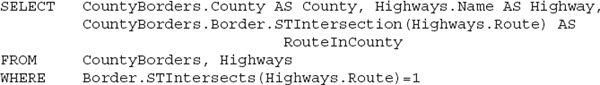
The results of the query of Listing 13-4 are shown on the grid in Figure 13-10. Hover the pointer over a segment to see the row to which it belongs. Each segment of the highway in the Spatial Results pane is identified by the name of the county and the name of the highway. The figure shows the labels on the segments of the two highways that lie in Los Angeles County.
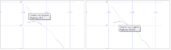
Figure 13-10 Viewing the intersections of US 101 and US 5 with various counties in California
The results of the same query in text format are shown in the table that follows. The
RouteInCounty column is the LINESTRING feature that belongs to the highway and is contained within the corresponding county. It’s a very long string and only part of it is shown on the printed page; US 101 is made up of 784 vertices and US 5 is made up of 1,745 vertices.
Joining Tables on Geo-Coordinates
The GEO sample database contains a table with geo-coded cities all over the states, the USCities table, but the USCities table contains no county information—just the state each city belongs to through a pointer to the USStates table. The CountyBorders table, on the other hand, contains the county borders in the state of California. Because both tables contain geographical data, you can associate them. To do so, you’re going to use the
STContains() method of a geography instance, which accepts another geography instance as an argument and returns 1 if the second instance is contained within the first instance. Obviously, the first instance must be a polygon. The second instance can be a line, a polygon, or a point. In the case of polygons and lines, the method will return 1 if the entire feature lies within the polygon to which the method applies.The
STContains() method enables you to retrieve the cities whose geo-coordinates fall within the polygons that outline the various counties. Here’s the statement that retrieves the cities and the counties they belong to:
The result of this query is similar to the following, depending on the number of counties and cities you have added to the corresponding tables:
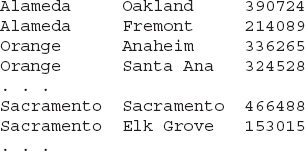
The results are sorted by county and by city name within each county. (The ellipses indicate additional cities in the same county.)
Additional Spatial Features
The methods discussed so far are the core of SQL Server’s spatial extensions, and these are the methods you will use to process geo-coded data in the context of preparing datasets for mapping applications. There are additional methods for specialized operations, which you can look up in the documentation. A few of the remaining methods, which seem to be useful in mapping applications, are presented in the section.
Extracting a Line’s Vertices
It’s quite possible that you have stored a line in a
geography column but no longer have access to the coordinates of the points you used to construct it. Or, you may have obtained the line definition in binary format. You can always retrieve the line’s vertices as text with the STAsText() method, but you will have to write some serious parsing code in T-SQL to extract individual points. A better alternative is to use the STPointN(i), which returns the ith vertex of the line or polygon to which it’s applied. The method’s argument is the index of the vertex you’re requesting and the value 1 corresponds to the first vertex. Unlike JavaScript, the first index in SQL Server collections starts at 1, not 0.Here’s a practical application of the
STPointN() method. As mentioned earlier in this chapter, the order in which vertices are specified in the definition of a polygon makes an enormous difference. Polygon vertices should be listed in a clockwise fashion; otherwise, they’re considered holes. If a polygon in your data has been defined backwards, you can reverse the order of its vertices by iterating through its vertices with the STPointN() method and create a new Well-Known Text representation for the reverse polygon. Listing 13-5 shows a SQL procedure that reverses the polygon representing the county of Alameda.Listing 13-5 Reversing the order of vertices in a POLYGON feature
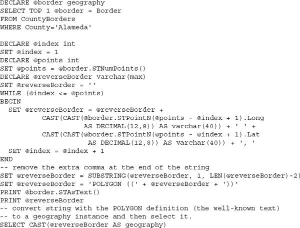
The last statement in the script selects the reversed polygon as a geography instance. In the Spatial Results tab, you will see that the county of Alameda has become a hole in the global map. You will find the query of Listing 13-5 in the
ReversePolygon.sql script in the support material of this chapter.Valid Geography Instances
All instances stored in a
geography column must be valid; otherwise, you won’t be able to process them with the usual spatial methods. However, SQL Server will accept invalid instances, as long as their definition is syntactically correct. If you specify a POLYGON primitive made up of points with the correct syntax, SQL Server will accept it and generate a binary representation of it. The polygon may still be invalid for many different reasons. A polygon with two vertices, for example, can be stored in a geography column, but it’s not a valid polygon. This polygon has no area!The
IsValid() method accepts a geography instance as an argument and returns 1 if its argument represents a valid geography, 0 otherwise. Figuring out what’s wrong in a polygon with many vertices by examining its definition is practically out of the question. Use the IsValidDetailed() method instead, which will give you a clue as to what’s wrong with your polygon and then try to fix it. As mentioned, many conditions may result in an invalid geography and they’re listed in SQL Server’s documentation at http://msdn.microsoft.com/en-us/library/hh710083.aspx.Another related method is
MakeValid(), which accepts as an argument the definition of an invalid geography and fixes it. The process of converting an invalid instance into a valid one may “slightly” shift the vertices of the shape. If you can’t figure out what’s wrong with your instance so that you can fix the raw data, the MakeValid() method is your best bet. The following statement was used to fix one of the county borders in the CountyBorders table:The
IsValid() method is an OCG method, while the other two extended methods, IsValidDetailed() and MakeValid(), are provided by SQL Server.The Union Operator with Shapes
Another interesting aspect of the spatial data is the union operation. With other data types, the
UNION operator combines the results of two or more queries, as long as all queries return the same number of columns and the data types of the columns match. The UNION operator can’t be used with spatial data. Instead, there’s an STUnion() method that combines spatial data into a single entity.To explore this
STUnion() method, let’s use the CountyBorders table with the outlines of the counties in California. The shape of California is the union of the shapes of the counties that make up the state. The STUnion() method combines the geography feature to which it is applied and another geography feature that’s passed as an argument to the method. To combine a few counties, start with the first one and then extend it by adding another county’s outline with the STUnion() method. The following statements attempt to reconstruct the state of California as the union of its counties: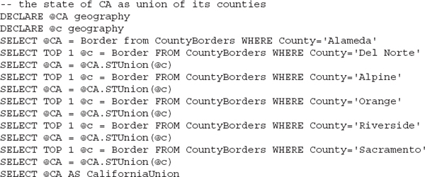
The statements shown here gradually build the outline of California by combining the polygons that correspond to individual counties. The variable
@CA represents a multi-polygon structure, as you can see in Figure 13-11, that shows the @CA variable in the Spatial Results pane, and it’s made up of the individual county polygons. The figure shows a few of the counties only. Note that most of them are easily distinguishable. The counties of Riverside and Orange at the lower-right corner of the tab, however, are totally joined because they have a common border. Add all counties to the @CA variable and you’ll end up with a polygon that has the exact same shape and size as the state of California.
Figure 13-11 The union of the polygons of the California counties
If you request the total area of the
@CA variable with the statement:T-SQL will return the value 31,161,176,910.9897, which is the sum of the areas of the counties added to the
@CA variable. If you include all counties in the query, you’ll get the total area of California.Approximating Lines
As you recall from Chapter 17, the Directions service returns approximate paths. The route from Manhattan to Chicago, for example, includes every turn along the way. When this path is placed on the map, however, and users view the map at a state level, there’s no need to render the complete path. The details of the route are not visible at that zoom level. You also learned how to approximate paths with the
Encode() method of the google.maps.geometry.Poly library. You used the Encode() method in Chapter 10 to reduce the size of a line’s representation. SQL Server provides a similar method to approximate both lines and polygons, and it’s described in this section.A path can be approximated with another path made up of fewer points. The approximation is based on a path’s vertices, but it doesn’t include all of them. Actually, it doesn’t include any of the original vertices; it’s made up of a smaller number of vertices that approximate the original path. This approximation is achieved with a famous algorithm in computational geometry, the Douglas-Peucker algorithm. The details of the algorithms are quite interesting, and you can easily find them on the Web, if you wish. SQL Server provides a method for approximating lines and shapes with the Douglas-Peucker algorithm, through the
Reduce() method. As you can see from its name, this method isn’t part of the OGC standard; it’s a SQL Server extended method, and you may find it quite useful in certain applications. If you want to further explore this algorithm, or implement your favorite language, you can find an interesting article that explains how it works with an animation at http://www.gitta.info/Generalisati/en/html/GenMethods_learningObject3.html.The
Reduce() method is applied to a geography feature (line or polygon) and accepts a maximum tolerance as an argument. The smaller the tolerance, the closer to the original shape is the approximation. The tolerance is specified in meters and its value depends on the type of feature you’re approximating. Let’s perform three different approximations of the polygon that outlines California. Figure 13-12 shows this polygon approximated with the following statement and with three different settings of the tolerance argument.
Figure 13-12 Approximating the state of California with the
Reduce() method at three different tolerance settingsThe following are the statements that produced the shapes shown in Figure 13-12:

As is evident from the figure, the tolerance value depends on the actual size of the shape and the acceptable distortion. You will probably experiment with the value of the argument to the
Reduce() method to find the most suitable value for the application at hand.To understand the meaning of tolerance in the Douglas-Peucker algorithm, you need to understand how the algorithm works in broad strokes. The Douglas-Peucker algorithm starts by approximating the path with a straight line, which has the same two endpoints as the path. Then, it locates the point along the path that lies the furthest away from the approximating line. This is the point that will have the most profound effect on the shape, if added to the approximation. If the distance of this point from the approximating line exceeds the tolerance, it’s added to the approximating line. Now the original path is approximated with two line segments and the algorithm continues with the two line segments on either side of the point that was added. It finds the two points that would have the most significant effect on the approximation of the two segments and, if they exceed the tolerance, it adds them to the approximating line. The algorithm continues by breaking the approximating line into two segments and adding (if needed) the point that will reduce the approximation error the most.
If you increase the tolerance too much, you’ll end up with a very rough sketch of the original line or shape, as you can see in Figure 13-12. Even this extremely rough approximation, though, may be useful in certain situations. It could simplify the first pass of a query that involves too many points or too many shapes. If you look at the last approximation of California’s shape, you’ll realize that it could be the ideal outline for a PowerPoint presentation, or similar application.
Converting Geography Features into JSON Objects
In this chapter, you learned a lot about SQL Server’s spatial features. You know how to store geospatial data into a database and retrieve it as needed, instead of maintaining numerous JSON arrays or KML files. Before ending this chapter, I should make the connection between the knowledge you acquired in this chapter with the scripts you use to create web pages with interactive maps.
In all scripts created so far in the book, the necessary data was embedded into the script. This is neither a JavaScript requirement, nor is it always the best approach. Even so, you should be able to extract the desired data from SQL Server and convert them to a format suitable for processing with JavaScript. To use the data, you should write queries that retrieve the desired data and then convert it to arrays of custom objects. The query in Listing 13-6 creates an array of JSON objects that represent the airports in the World Airports table of the GEO database.
Listing 13-6 A T-SQL script that creates a JSON array of custom objects with the data from the World Airports table
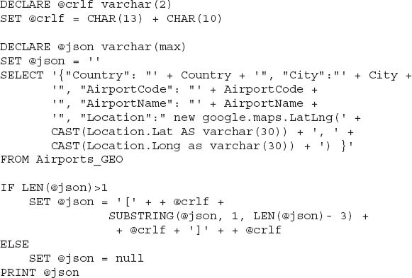
The preceding statements will generate the following output when executed against the World Airports table of the GEO sample database:
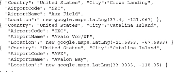
You will find the query of Listing 13-6 in the
Airports2JavaScript.sql script in the support material of this chapter. This JavaScript array can be used as is in a script. You can embed this array definition in a script, or store it at your server and reference it in the script with a <script> directive. The most flexible approach is to download the file at the client as needed, with the XMLHttpRequest object. This object allows you to download XML and/or JSON files in your JavaScript code as needed and use them just like any array embedded in the script. The XMLHttpRequest object is discussed in detail in Chapter 15.Listing 13-7 shows another interesting script, which converts the outline of a county from a
POLYGON structure into a JavaScript array of coordinates. The query starts by extracting from the CountyBorders table the polygon that outlines the county of Alameda. Then, it iterates through the polygon’s vertices, reads each vertex’s coordinates, and gradually builds a string, which is the definition of the JavaScript array. The script uses the shape’s STNumPoints() method to extract the number of points in the polygon, and the STPointN() method to extract the coordinates of each vertex.Listing 13-7 A T-SQL script that transforms the coordinates of a POLYGON geography feature into an array of
LatLang objects
A segment of the output of the preceding query is shown next. It’s a JavaScript array of
LatLng objects that can be used as a line’s or polygon’s path to render Alameda’s polygon on the map.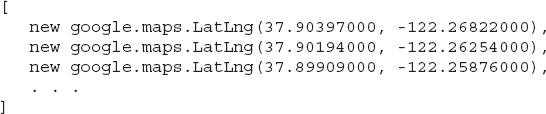
The SQL script of Listing 13-7 can be found in the
Polygon2JavaScript.sql file in the chapter’s support material.Summary
In the last few chapters, you have seen how to annotate maps with markers and shapes. These items are placed on their own layer on top of the map, and you know how to persist them in KML format, as well how to store them in a database. You also know how to query the database and retrieve the desired data in many different formats, depending on your application requirements. In Chapter 15, you will see how to expose the database data as web services and access these services from within your script.
In the following chapter, you build a Windows application for annotating maps with data that resides in a database. You will do so by selecting the items you want to place on the map, and then the application will generate a stand-alone web page with the appropriate script and data, which can be presented to end users.
..................Content has been hidden....................
You can't read the all page of ebook, please click here login for view all page.