This chapter is devoted to the application of the single contact point transient tire models as developed in the preceding chapter. The applications demonstrate the effect of the tire relaxation length on vehicle dynamic behavior. In Chapter 6 a similar first-order tire model was used to study the wheel shimmy phenomenon, cf. Eqn (6.7) with a = 0.

8.1 Vehicle Response to Steer Angle Variations

In Chapter 1, Section 1.3.2, the dynamic response of the two-degree of freedom vehicle model depicted in Figures 1.9, 1.11 to steer angle input has been analyzed. As an extension to this model, we will introduce tires with lagged side force response. The system remains linear and we may use Eqn (7.18). The relaxation length will be denoted by σ. We have the new set of equations:

(8.1)

(8.2)

(8.3)

(8.4)

(8.5)

(8.6)

Figure 8.1 presents the computed frequency response functions, which hold for the extended system, for different values of the relaxation length. In Figure 8.2 the corresponding step response functions are depicted. The diagrams show that the influence of the tire lag on the vehicle motion is relatively small. At higher values of speed, the effect diminishes and may become negligible.

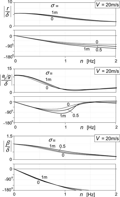
FIGURE 8.1 Frequency response of yaw rate, lateral acceleration, and vehicle side slip angle to steer angle of vehicle model featuring tires with lagging side force response, cf. Figure 1.15.

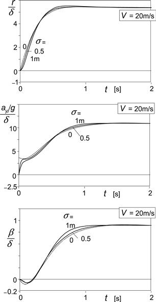
FIGURE 8.2 Step response of yaw rate, lateral acceleration, and vehicle side slip angle to steer angle of vehicle model featuring tires with lagging side force response.

However, for closed-loop vehicle control systems, the additional phase lag caused by the relaxation lengths may significantly affect the performance.

An interesting effect can be seen to occur near the start of the step response functions. With the relaxation length introduced, the responses appear to exhibit a more relaxed nature. The yaw rate response shows some initial lag.

8.2 Cornering on Undulated Roads

When a car runs along a circular path over an uneven road surface, the wheels move up and down and may even jump from the road while still the centripetal forces are to be generated. Under these conditions, the wheels run at slip angles which may become considerably larger than on a smooth road. Consequently, on average, the cornering stiffness diminishes. This phenomenon was examined in Chapter 5, Section 5.6, where the stretched string model was found to be suitable to explain the decrease in cornering stiffness if the string relaxation length is made dependent on the varying wheel load to imitate the model provided with tread elements, cf. Figure 5.51.

These tire models, however, are considered to be too complicated to be used in vehicle simulation studies. Instead, we will try the very simple transient tire model as discussed in Section 7.2.1 and compare the results with experimental findings. First, the small slip angle linear model will be considered. We use Eqn (7.20) which may be given the form:

(8.7)

where s denotes the traveled distance and ds = V_xdt. The slip angle is assumed to be constant while the vertical load varies periodically.

(8.8)

Essential is that both the cornering stiffness and the relaxation length vary with the vertical load:

(8.9)

Figure 8.3 illustrates the situation.

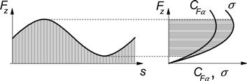
FIGURE 8.3 Cornering stiffness and relaxation length varying with wheel load.

The loss in cornering power can be divided into the ‘static’ loss and the ‘dynamic’ loss. The static loss arises due to the curvature of the cornering stiffness vs wheel load characteristic. A similar loss has been experienced to occur as a result of lateral load transfer in the analysis of steady-state cornering of an automobile, cf. Figure 1.7. Figure 8.4 explains the situation at sinusoidally changing wheel load.

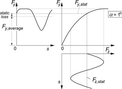
FIGURE 8.4 The static loss in average side force due to the curved force vs load relationship.

As will be shown in the analysis below, the dynamic loss appears to be attributed to the rate of change of the relaxation length with wheel load. This, of course, can only occur because of the fact that the cornering stiffness varies with wheel load since that rate of change forms the input in Eqn (8.7). Apparently, with both F_y and σ being dependent on F_z while α in the present analysis only affects F_y, the phenomenon is nonlinear in F_z and linear in α.

If we assume a quadratic function for the C_Fα vs F_z relationship with the curvature bC_Fα_o

(8.10)

the static loss can be simply found to become

(8.11)

The occurrence of the dynamic loss may be explained by assuming a linear variation of both the cornering stiffness and the relaxation length with load:

(8.12)

Equation (8.7) becomes herewith:

(8.13)

or simplified:

(8.14)

with z = cF_z, y = F_y, β = eα/c. Consider a truncated Fourier series approximation of the periodic solution:

(8.15)

and its derivative:

(8.16)

while the input

(8.17)

Substitution of (8.15, 8.16, 8.17) in (8.14) and subsequently making the coefficients of corresponding terms in the left and right members equal to each other yields for the average output:

(8.18)

The average side force F_y_,ave expressed in terms of the original quantities now reads as

(8.19)

For large F_z amplitudes and short wavelengths λ = 2π/ω_s the formula shows that the dynamic loss approaches 50% of the side force generated on smooth roads. As we will see, this finding agrees very well with simulation and test results.

The aligning torque variation may be computed as well. In their study, Takahashi and Pacejka (1987) employed the equation based on the string concept and added the gyroscopic couple. We obtain according to Eqns (5.135) and (5.178), the latter expression corresponding with (7.49):

(8.20)

and

(8.21)

The total moment responding to the slip angle becomes

(8.22)

Experiments have been conducted to assess the relevant parameters of a 195/60R14-87H tire at various values of the vertical load. The diagrams of Figure 8.5 present the characteristics for the relaxation length, the cornering stiffness, and the aligning stiffness. The relaxation length was determined by curve fitting of the data obtained from a swept sine steering oscillation test at a speed of 30 km/h in the frequency range of 0–2 Hz. The gyroscopic coefficient C_gyr was assessed in a similar test but conducted at a speed of 170 km/h. The resulting value turns out to be C_gyr = 3.62 × 10⁻⁵ s² that corresponds to the nondimensional coefficient c_gyr ≈ 0.5, cf. Eqn (5.179).

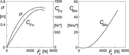
FIGURE 8.5 Load dependency of tire parameters according to measurements and third-degree polynomial fits.

To assess the validity of the calculated force and moment response to load variations experiments have been carried out on a 2.5-m drum with a special test rig at the Delft University of Technology. The wheel axle can be moved vertically while set at a given slip angle. The side force and moment measured at that slip angle have been corrected for the responses belonging to a slip angle equal to zero.

In Figure 8.6, in the left-hand diagrams, the test results are presented. The wheel axle is vertically oscillated with frequencies up to 8 Hz and with an amplitude that corresponds to the ratio of amplitude and mean value of the wheel load equal to 0.9. The wheel runs at a constant small slip angle of one degree with a speed of 30 km/h. The response at the low frequency of 0.5 Hz may be considered as quasi-static and varies periodically, practically in phase with the axle motion. To enable a proper comparison at the different frequencies, the responses have been plotted against traveled distance divided by the current wavelength. The right-hand diagrams show the corresponding calculated responses. In view of the very simple set of equations that have been used, the agreement between test and model can be considered to be very good. Calculations conducted with the stretched string model of Section 5.6 were not much better. Only the moment responses turned out to be a little closer to the experimental findings. In the responses, two major features can be identified. First, we observe that the responses show some lag with respect to the input that grows with increasing frequency n which means: with decreasing wavelength λ. Second, and more important, we have the clear drop in average value of the side force which becomes larger at increasing frequency. After subtracting the static drop that occurs at the lowest frequency, the dynamic loss remains.

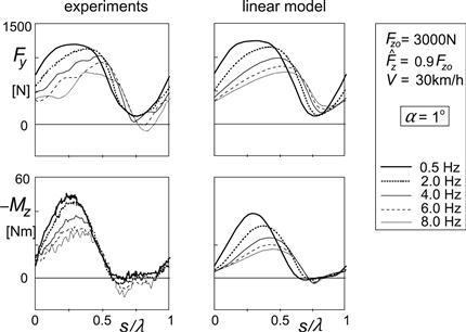
FIGURE 8.6 Side force and aligning torque response to wheel load variation at small slip angle.

In Figure 8.7 the static and the dynamic parts of the decrease of the average side force, as a ratio to the side force at zero vertical load amplitude, have been plotted versus frequency or wavelength for different input amplitude ratios. The model shows reasonable agreement with the experimental results. It has been found that the correspondence becomes a lot better when the speed is increased to 90 km/h. Then, the wavelength is three times larger and a better performance of the model prevails. The curve of Figure 8.7 that holds for the amplitude ratio 0.95, where the tire almost loses contact, appears to approach the value of ca. 0.5 when the frequency increases to large values. This indeed corresponds to the analytical result established by Eqn (8.19). On the other hand, the more advanced model of Section 5.6 predicts a possibly even larger reduction at the verge of periodic lift-off; cf. Figure 5.51 where the wavelength could be diminished to levels as small as the static contact length 2a_o.

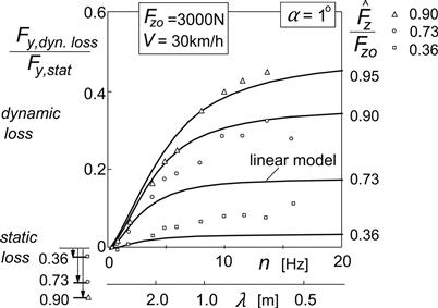
FIGURE 8.7 Dynamic side force loss at a small slip angle for different load amplitude ratios.

It may be obvious that an analogous model, Eqn (7.9) with , can be used for the in-plane non-steady-state response to vertical load variations. Without special measures it is virtually impossible to maintain a certain level of the longitudinal slip κ at varying contact conditions. At a fixed braking torque, the average longitudinal braking force remains constant when the wheel keeps rolling. When the wheel runs over an uneven road surface and the wheel load changes continuously, the effect of the tire lag is an increased average level of the longitudinal slip ratio. Applications of the single contact point in-plane transient model follow in Sections 8.3 and 8.5 where problems related with tire out of roundness and braking on undulated roads are discussed.

The theory can be extended to larger values of slip if the nonlinear model according to Eqns (7.25, 7.26) is employed. The equations may be used here in the form:

(8.23)

with

(8.24)

which quantity is a function of both the wheel load F_z and the transient slip angle or deformation gradient α′. It reduces to the relaxation length σ₀ (=σ at α′ = 0) when α′ tends to zero and F_y/α′to C_Fα. Obviously, offsets of the side force vs slip angle characteristic near the origin have been disregarded here. The transient slip angle follows from

(8.25)

The side force and moment are obtained by using the steady-state characteristics:

(8.26)

(8.27)

With the gyroscopic couple, cf. Eqns (8.21), (7.5) and (5.179)

(8.28)

the total moment becomes

(8.29)

The steady-state characteristics as measured on the road at a number of wheel loads are presented in Figure 8.8.

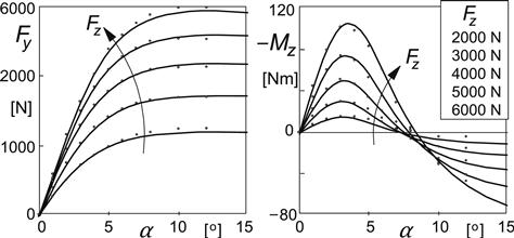
FIGURE 8.8 Steady-state side force and aligning torque characteristics as measured on the road.

As has been noted in Section 7.2.3 the assessment of requires some attention. In the investigation done by Pacejka and Takahashi (1992) and Higuchi (1997), the solution was obtained through iterations. Alternatively, we may use information from the previous time step to assess . When the load is rapidly lowered, violent vibrations may occasionally show up in the solution.

With this nonlinear model, simulations have been done and experiments have been carried out for a slip angle equal to six degrees. Plots of the resulting responses are shown in Figure 8.9. The model appears to be successful in predicting the side force variation caused by the wheel load excitation at different frequencies. The load amplitude ratio of 0.83 gave rise to full sliding in certain intervals of the periodic motion. This can be seen to occur when the force signal touches the curve representing the maximally achievable side force μF_z. In this respect, the model certainly performs well which cannot be said of the alternative model governed by Eqn (7.20) with F_y,ss calculated with Eqn (8.26) where α′ is replaced by α. This model gives rise to a calculated force response that exceeds this physical limit when the load approaches its minimal value due to the phase lag of the response. The dynamic loss of the average side force follows a tendency similar to what was found with the linear model at small slip angles. The result obtained at a constant slip angle of six degrees is shown in the diagram of Figure 8.10. The correspondence with the experimental outcome becomes even better than in the case of a slip angle equal to one degree, Figure 8.7.

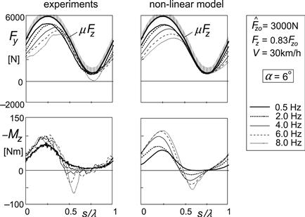
FIGURE 8.9 Side force and aligning torque response to wheel load variation at large slip angle.

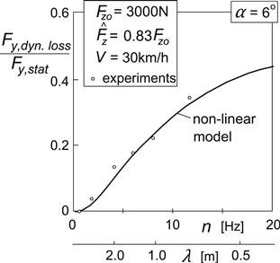
FIGURE 8.10 The dynamic loss at a large constant slip angle and a large load amplitude ratio.

Very similar results have been obtained with the more robust enhanced model of Section 7.3. The difference is that a small dynamic force acts on the little mass of the contact patch used in the model. This causes the ground force to be slightly different from the force felt at the wheel rim. It is, of course, the ground force that cannot exceed the physical limit mentioned above.

8.3 Longitudinal Force Response to Tire Nonuniformity, Axle Motions, and Road Unevenness

In this section, the response of the axle forces F_x and F_z to in-plane axle motions (x, z), road waviness and tire nonuniformities will be discussed. For a given tire–wheel combination, the response depends on rolling speed and frequency of excitation. This dependency, however, appears to be of much greater significance for the fore and aft force variation F_x than for the vertical load variation F_z.

The vertical force response has an elastic component and a component due to hysteresis. A similar mechanism is responsible for the generation of (at least an important portion of) the rolling resistance. The hysteresis (damping) part of the vertical load response appears to rapidly decrease to almost negligible levels at from zero increasing forward speed, cf. Pacejka (1981a) and Jianmin et al. (2001). We simplify the relationship between normal load F_z and radial tire deflection ρ using the radial stiffness C_Fz:

(8.30)

In Chapter 9, tire inertia and other influences will be introduced to improve the relationship at higher frequencies and shorter wavelengths of road unevennesses.

A coupling between vertical deflection variation and longitudinal force appears to exist that is due to the resulting variation of the effective rolling radius of the tire.

For the non-steady-state analysis, we will employ the linear Eqn (7.9) that may take the form with V = V_x (assumed positive):

(8.31)

The input is the longitudinal slip velocity that is defined as

(8.32)

Obviously, the effective rolling radius r_e plays a crucial role here.

8.3.1 Effective Rolling Radius Variations at Free Rolling

For a wheel with tire that is uniform and rolls freely at constant speed over an even horizontal road surface, the tractive force required is due to rolling resistance alone. Under these conditions, the effective rolling radius r_e is defined to relate speed of rolling Ω with forward speed V:

(8.33)

The center of rotation of the wheel body S lies at a distance r_e below the wheel spin axis. As has been discussed in Chapter 1, by definition, this point which can be imagined to be attached to the wheel rim, is stationary at the instant considered if the wheel rolls freely (cf. Figure 8.11 with slip speed V_sx = 0). In general, the effective rolling radius changes with tire deflection ρ. We may write

(8.34)

with r_f denoting the free (undeformed) radius that may vary along the tire circumference due to tire nonuniformity. We have for the loaded radius:

(8.35)

Figure 8.12 shows variations of the effective rolling radius r_e and the loaded radius r as functions of wheel load F_z for two different tires at different stages of wear and at different speeds as measured on a drum surface of 2.5-m diameter. The reduction of the effective rolling radius f (ρ) with respect to its theoretical original value r_f at zero wheel load (ρ = 0) that has been deduced from diagram 8.12 has been presented in Figure 8.13. The influence of a change in tread depth has been shown. The slope η and the coefficient ε indicate the influence of changes in deflection and tread depth near the nominal load.

FIGURE 8.11 The rolling wheel subjected to longitudinal slip (slip speed V_sx).

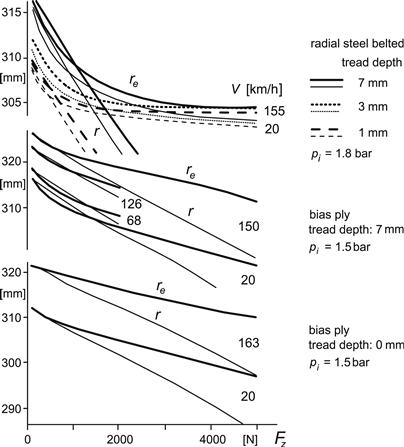
FIGURE 8.12 Tire effective rolling radius and loaded radius as a function of wheel load, measured on 2.5-m drum at different speeds and for different tread depths and tire design. Note the different scales for the radial and bias-ply tire radii.

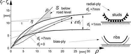
FIGURE 8.13 Reduction of effective rolling radius r_e with respect to tire free radius r_f due to tire radial deflection ρ and tread depth change d_t. Situation at nominal load, F_z_o = 3000 N, has been indicated by circles.

Figure 8.14 tries to explain the observation regarding the location of the slip point S: possible locations have been indicated. At zero wheel load, S lies at road level or a little lower (due to air and bearing resistance which slows the wheel down at the expense of some slip). A small wheel load causes a number of the originally radially directed tread elements to assume a vertical orientation. The rotation of these tread elements is lost which causes the effective radius to become smaller. Point S may then turn out to lie above road level! At higher loads, we get the more commonly known situation of S located below road level. It has been assumed here that the belt with radius r_c is inextensible. Then, when the lower tread elements have a vertical orientation and translate backwards with respect to the wheel center, the wheel will in one revolution cover a distance equal to the circumference of the belt. This means that the effective rolling radius equals the radius of the belt. When the tire possesses a ribbed tread pattern, it is expected that due to the greater coherence between rib elements in comparison to the independent studs of the radial-ply tire, some rotation still occurs in the ribs in the contact zone which increases the effective radius and pushes point S earlier below the road surface. This theory seems to be supported by the curves of the new bias-ply tire. The degree of effective incoherence ε is estimated for the radial-ply tire to be equal to ca. 0.9 and for the bias-ply tire equal to 0.2 at the rated load. Because we have plotted in Figure 8.13 the reduction of the effective radius with respect to the free unloaded radius: r_f − r_e, the decrease of r_e due to the wearing off of the tread rubber is not shown directly. Only the indirect effect of tread wear is shown through the tread incoherence parameter ε. If due to the vertical tire deflection the tread band is compressed and has decreased in circumference, the effective radius diminishes. This property, which is more apparent to happen with the bias-ply tire, is partly responsible for the slope of the curves shown at larger vertical deflections. This slope, denoted with η, is estimated to be equal to about 0.1 for the new radial-ply tire with an almost inextensible belt and 0.4 for the new bias-ply tire at their nominal load.

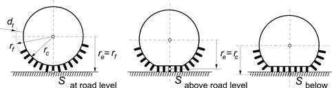
FIGURE 8.14 Location of the center of rotation, the slip point S, at three different radial deflections.

The analysis will be kept linear and we assume small deviations from the undisturbed condition. In the neighborhood of this average state, we write for the effective radius, the loaded radius, and the radial deflection:

(8.36)

Small deviations from the undisturbed condition are indicated by a tilde. Variation of the free radius may occur along the circumference of the tire. This kind of nonuniformity (out of roundness) is composed of two contributions: one is due to variations of the carcass radius r_c and the other due to variations of the tread thickness d_t. We have

(8.37)

The value of out of roundness is considered to be present at the moment considered along the radius pointing to the contact center. The following linear relation between the effective radius variation and the imposed disturbance quantities is found to exist:

(8.38)

The observation that a reduction in thickness of the tread rubber of a radial-ply tire produces a decrease in effective rolling radius (at F_z_o), amounting to only a small fraction of the reduction in tread depth, is reflected by the factor (1 − ε) in the right-hand expression of (8.38). The coupling coefficient η is relatively small for belted tires. In contrast to bias-ply tires, the effective rolling radius of a belted tire does not change very much with deflection once the initial tread thickness effect (at small contact lengths with tread elements still oriented almost radially) has been overcome.

8.3.2 Computation of the Horizontal Longitudinal Force Response

The horizontal force response on undulated roads is composed of the following three contributions: the horizontal component of the normal load, the variation of the rolling resistance, and the longitudinal force response to the variation of the wheel longitudinal slip. The horizontal in-plane force designated with X becomes, with linearized variations, cf. Figure 8.15,

(8.39)

with F_r_o denoting the average rolling resistance force. For this occasion, it is assumed that the variation in rolling resistance force is directly transmitted to the tread through changes in vertical load. We write

(8.40)

where the variation of the vertical load results from variations in deflection and possibly from changes in radial stiffness along the tire circumference:

(8.41)

or expressed in terms of the variation in radial static deflection:

(8.42)

we may write

(8.43)

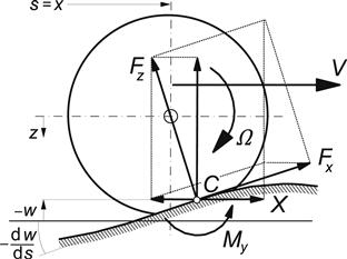
FIGURE 8.15 In-plane excitation by road unevenness and by vertical and fore and aft axle motions.

The variation of the tangential slip force becomes, with the transient longitudinal slip ,

(8.44)

where the tire deflection u follows from Eqn (8.31). The longitudinal slip velocity appearing as input in (8.31) is governed by Eqn (8.32). With the variations in forward velocity, speed of revolution, and effective rolling radius, we find in linearized form

(8.45)

The variation of the effective rolling radius follows from (8.38), where the deflection is a result of the combination of wheel vertical displacement, tire out of roundness, and road height changes:

(8.46)

The wheel angular velocity results from the dynamic equation

(8.47)

in which I_w denotes the wheel polar moment of inertia (including a large part of the tire that vibrates along with the wheel rim if the frequency lies well below the in-plane first natural frequency, cf. Chap. 9).

The moment M_y acts about the transverse axis through the contact center C, Figure 8.15, and is composed of the part due to rolling resistance and a part due to eccentricity of the tread band which constitutes the first harmonic of the tire out of roundness. This latter part runs 90 degrees ahead in phase with respect to the loaded radius variation that is sensed at the contact center. With subscript 1 referring to the first harmonic we have

(8.48)

The rolling resistance moment M_r is here supposed to be directly connected with the rolling resistance force F_r which is a simplifying assumption that has a negligible effect on the resulting responses. As a result, the rolling resistance components cancel out in the right-hand member of Eqn (8.47). This equation now reduces to

(8.49)

Collection of the relevant Eqns (8.31, 8.38–8.43, 8.45) and elimination of all variables, except the input quantities

(8.50)

and the output and, for now, also and , yields the following Laplace transformed representation of the horizontal force variation with s designating the Laplace variable or iω:

(8.51)

where with (8.38) and (8.46) we have the variations of effective radius and tire deflection:

(8.52)

and

(8.53)

From this expression (8.51) of the combined response, the individual transfer functions or the frequency response functions to the various input quantities may be written explicitly. For the latter functions to obtain, we simply have to take the coefficients of one of the input variables (8.50) in (8.51), after (8.52) and (8.53) have been inserted in (8.51), and replace s by iω or iΩ_o depending on the type of input variable.

Figure 8.16 presents both theoretical and experimental data, the latter being obtained from tests performed on a 2.5-m drum test stand provided with a specially designed rig (Pacejka, Van der Berg and Jillesma 1977). The parameters of the tires tested have been listed in Table 8.1.

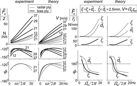
FIGURE 8.16 Experimental and theoretical frequency response plots of the longitudinal force F_x to vertical axle oscillations z and to out of roundness (1^st harmonic of variations in carcass radius r_c or in tread thickness d_t). Average vertical load F_z_o = 3000 N.

TABLE 8.1 Tire In-plane Parameter Values for the Radial and Bias-ply Tires

Radial steel-belted (p_i =1.8 bar, tread depth (at ) = 6.5 mm)

I_w = 0.8 (z) or 1.1

kgm², r_f_o = 0.315 m, r_o ≈ 0.3 m, η = 0.1, ε = 0.6,

σ_κ = C_Fx/C_Fκ, C_Fx = 565 kN/m, C_Fκ = 80 kN (500 kN at

= 2.5 mm),

F_z_o = 3000 N, F_r_o = 25 N, C_Fz = 133 kN/m, A_r = 0.0083

Bias-ply (p_i = 1.5 bar, tread depth = 6.5 mm)

I_w = 0.8 (z) or 1.1

kgm², r_f_o = 0.325 m, r_o ≈ 0.3 m, η = 0.4

σ_κ = C_Fx/C_Fκ, C_Fx = 1000 kN/m, C_Fκ = 45 kN

F_z_o = 3000 N, F_r_o = 60 N, C_Fz = 190 kN/m, A_r = 0.02

The response to z has been found by moving the axle up and down by means of a hydraulic actuator. The variation in carcass radius r_c has been achieved by mounting a reasonably uniform wheel and tire with 2.5-mm eccentricity on the shaft and subsequently balancing the rotating system. In this test, the axle was held fixed. The special arrangement resulted in a larger polar moment of inertia I_w (1.1 kgm²). The response to d_t variations could be obtained by partly buffing off the tire tread. On one side 5 mm less tread rubber remained with respect to the other side of the tire. As a side effect, the average slip stiffness C_Fκ increased. The new value was estimated. All tire parameters have been determined through special tests. Sometimes, slight changes of these values could result in a better match of the response data.

In general, a good correspondence with experimental results could be established. Also, the phase relationship, which is very sensitive to the structure of the model and changes in parameters, turns out to behave satisfactorily. A negative phase angle ϕ indicates that the response lags behind the input.

To explain these findings which turn out to be quite different for the two types of tires, we shall now analyze the responses to vertical axle motions z and out of roundness in greater detail.

8.3.3 Frequency Response to Vertical Axle Motions

After replacing in Eqn (8.51) the Laplace variable s by iω, with ω denoting the frequency of the excitation, we find for the response to vertical axle motions the following frequency response function with X = F_x:

(8.54)

with the nondimensional frequency:

(8.55)

and the speed-dependent damping ratio:

(8.56)

where the natural frequency of the tire–wheel rotation with respect to the foot print has been introduced:

(8.57)

An interesting observation is that an increase in slip stiffness or relaxation length decreases the nondimensional damping coefficient ζ. A higher speed V, obviously, produces more damping.

For the extreme case, ω → 0, we find as expected only the contribution to rolling resistance:

(8.58)

If we neglect the small contribution from the rolling resistance, the first term of (8.54) vanishes. The magnitude of the remaining term reduces to a simple expression if the frequency is considered to be small with respect to the natural frequency:

(8.59)

with V the speed of travel in m/s and n the frequency of the vertical axle motion in Hz. It is noted from Eqn (8.59) that the rise of the response in the lower frequency range with the frequency n and the speed V is in particular influenced by the magnitude of the factor η multiplied with the polar moment of inertia I_w. A small value of η, as with radial tires, is favorable which is obviously caused by the fact that then the change of effective rolling radius with deflection is very small so that rotational accelerations and accompanying longitudinal forces are almost absent. The coefficient of Vn in (8.59) for the radial-ply tire becomes 18.6 and for the bias-ply tire 74.5. This would mean that if the wheel with bias-ply tire that rolls at a speed of 10 m/s is oscillated vertically with an amplitude of 1 mm at a frequency of 10 Hz, the resulting longitudinal force gets an amplitude of 7.45 N.

At higher frequencies it can be shown that the curves for the magnitude of expression (8.54) reach a common maximum (for all V) at ω = ω_Ωo. The maximum response amplitude amounts to

(8.60)

This maximum is determined again primarily by the effective rolling radius gradient η but now multiplied with slip stiffness C_Fκ. For the radial tire, the maximum response becomes ca. 28 N/mm at the natural frequency 43 Hz and for the bias-ply tire this becomes ca. 64 N/mm at 57 Hz. Figure 8.17 shows both the amplitude and phase (lag) response calculated for the bias-ply tire. Figure 8.16 has already indicated that for the radial tire a much lower response is expected to occur.

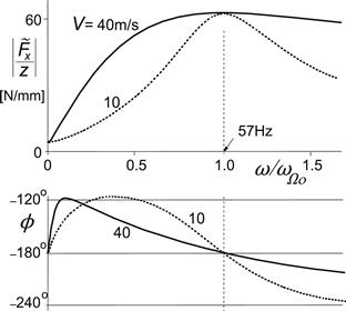
FIGURE 8.17 Theoretical frequency response function of the longitudinal force F_x to vertical axle motions z for the bias-ply car tire.

8.3.4 Frequency Response to Radial Run-out

From Eqn (8.51) we derive for the frequency response to radial (carcass) run-out considering only its first harmonic with frequency equal to the wheel speed of revolution ω = Ω (nondimensional frequency ν = Ω/ω_Ωo):

(8.61)

This expression differs in two main respects from the one for the response to axle vertical motions (8.54). First, we have now the factor 1 − η instead of η and, second, an additional term with F_z_o shows up which is due to the eccentricity, cf. Eqn (8.49). Figure 8.18 presents the response plots for the bias-ply tire.

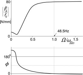
FIGURE 8.18 Theoretical frequency response curve of longitudinal force to tire out of roundness (1^st harmonic) for the bias-ply tire. The speed of travel V = r_eΩ.

For speeds very low, Ω → 0 the expression reduces to

(8.62)

The amplitude ratio attains a minimum near

(8.63)

which means for the radial tire, near the frequency 0.14 n_Ωo and, for the bias-ply tire, near 0.13 n_Ωo. With parameters corresponding to the experiment conducted (I_w = 1.1 kgm² resulting in natural frequencies of 36.5 and 48.5 Hz) we obtain for these frequencies 5.1 and 6.3 Hz, respectively. The minimum value appears to become very close to A_rC_Fz = 1100 and 3800 N/m, respectively. As can be seen in the upper right-hand diagram of Figure 8.16, the experimentally assessed curve also features such a dip in the low-frequency range and the accompanying sharp decrease in phase lead. At the natural frequency n_Ω0 (ν = 1), the amplitude ratio comes close to its maximum value. This maximum is approximately equal to

(8.64)

The second term by far dominates this expression. The radial tire attains 220 N/mm (at 36.5 Hz) and the bias-ply tire attains 80 N/mm (at 48.5 Hz). Compared with the maximum longitudinal force response to vertical axle motions, Eqn (8.60), we note a much stronger sensitivity of the radial tire to out of roundness (ca. 220 N/mm) than to vertical axle motions (ca. 28 N/mm). This is due to the factor 1−η occurring in (8.64) which in (8.60) appears as η. For the bias-ply tire with a much more compressible tread band, we have 80 N/mm versus 64 N/mm.

Exercise 8.1. Response to Tire Stiffness Variations

Derive from Eqns (8.51) to (8.53) the frequency response function of F_x to the static deflection variation , that is, to variations in radial tire stiffness, for fixed axle height, z = 0. Then release the vertical axle motion and find the frequency response function for z to . Consider Figure 8.19 that represents the simplified axle/wheel-suspension system. Small motions are considered so that only linear terms can be taken into account. Use the parameter values of the bias-ply tire of Table 8.1 and furthermore the values for the mass, the suspension stiffness, and the damping:

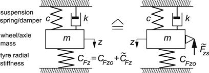
FIGURE 8.19 Wheel suspension/mass system excited by tire stiffness variations (Exercise 8.1).

Now find the total frequency response of F_x to for the released axle motion. It may be noted that the excitation by a variation of the radial stiffness is equivalent to the excitation by a vertical force:

representing the variation of the ‘static’ tire load at constant axle height while the tire rolls.

Exercise 8.2. Self-excited Wheel Hop

Investigate the stability of the fourth-order system of Figure 8.20 using the Hurwitz criterion (cf. Eqn (1.118)). Employ Eqns (8.31, 8.38, 8.45–8.47), assume M_y = 0, and consider a flat road and a uniform tire. Assess the range of the slope β of the wheel axle guidance surface where instability will occur for the undamped wheel suspension system. The effective rolling radius coupling coefficient η is the decisive parameter. Plot the stability boundary in the tan β versus η diagram. Vary η between the values 0 and 1. Indicate the areas where stability prevails. Take the parameter values:

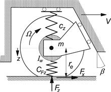
FIGURE 8.20 On the possibly unstable wheel hop motion (Exercise 8.2).

That a moderate oscillatory instability may indeed show up with such a system has been demonstrated experimentally in professor S.K. Clark’s laboratory at the University of Michigan in 1970.

8.4 Forced Steering Vibrations

A steering/suspension system of an automobile exhibits a rather complex configuration and possesses many degrees of freedom. A simplification is necessary to conduct a sensible analysis to gain insight into its general dynamic behavior and into the influence of important parameters of the system. Investigation of the steering mode of vibration requires at least the steering degree of freedom of the front wheel, possibly extended with the rotation degree of freedom of the steering wheel. For the sake of simplicity, one degree of freedom may be suppressed by holding the steering spring clamped at the node of the natural mode of vibration. Furthermore, we will consider the influence of two more degrees of freedom: the vertical axle motion and the longitudinal deflection of the suspension with respect to the steadily moving vehicle mass. The picture of Figure 8.21 shows the layout of system. Due to the assumed orthogonality of the system (wheel axis, kingpin, and road plane) the dynamically coupled horizontal motions (x, ψ) are not coupled with the vertical axle motion when small displacements are considered and tire contact forces are disregarded.

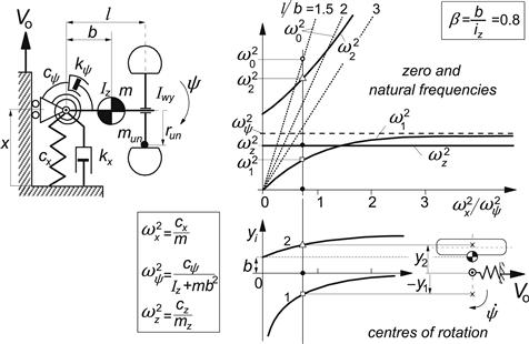
FIGURE 8.21 Configuration of a simple steering/suspension system and the resulting natural frequencies and vibrational modes.

First, we will examine the dynamics of the free system not touching the road. After that, the tire is loaded and tire transient models for the in-plane and out-of-plane behavior are introduced and the system response to wheel unbalance will be assessed and discussed.

8.4.1 Dynamics of the Unloaded System Excited by Wheel Unbalance

The simple system depicted in Figure 8.21 possesses two horizontal degrees of freedom: the rotation about the vertical steering axis, ψ, and the fore and aft suspension deflection, x. The figure provides details about the geometry, stiffnesses, damping, and inertia. The mass m represents the total mass of the horizontally moving parts. The length i_z denotes the radius of inertia: .

The wheel rim that revolves with a speed Ω is provided with an unbalance mass m_un (in the wheel center plane at a radius r_un). The centrifugal force has a component in forward direction:

(8.65)

The equations of motion of this fourth-order system read as

(8.66)

(8.67)

With damping disregarded, the magnitude of the frequency response function becomes

(8.68)

in which we have the zero frequency:

(8.69)

and the two natural frequencies:

(8.70)

where we have introduced the ‘uncoupled’ natural frequencies:

(8.71)

and the coupling factor:

(8.72)

For the analysis, we are interested in the influence of the fore and aft compliance of the suspension. In the right-hand diagram of Figure 8.21 the two natural frequencies have been plotted as a function of the longitudinal natural frequency ratio (squared), which is proportional to the longitudinal stiffness c_x, together with the constant vertical natural frequency and the zero frequency for three different values of f/b. In addition, the location of the two centers of rotation according to the two modes of the undamped vibration has been indicated.

The two steer natural frequencies ω₁ and ω₂ increase with increasing longitudinal suspension stiffness. The lower natural frequency with a center of rotation located at the inside of the kingpin approaches the uncoupled natural frequency ω_ψ.

From (8.69) it is seen that a zero does not occur if the unbalance arm length l lies in the range 0 < l < b which does not represent a usual configuration. For the normal situation with b > 0 the zero frequency line may cross the second natural frequency curve if l is not too large. If the two frequencies coincide, the second resonance peak of the steer response to unbalance will be suppressed. In that case, the unbalance force line of action passes through the center of rotation of the higher vibration mode.

It may be noted that the situation with contact between wheel and road can be simply modeled if the wheel is assumed to be rigid. The same equations apply with inertia parameters adapted according to the altered system with a point mass attached to the axle in the wheel plane. The point mass has the value I_w/r² where I_w denotes the wheel polar moment of inertia and r the wheel radius.

8.4.2 Dynamics of the Loaded System with Tire Properties Included

In a more realistic model, the in-plane and out-of-plane slip, compliance, and inertia parameters should be taken into account. A possible important aspect is the interaction between vertical tire deflection and longitudinal slip which may cause the appearance of a third resonance peak near the vertical natural frequency of the wheel system. The longitudinal carcass compliance gives rise to an additional natural frequency around 40 Hz of the wheel rotating against the foot print (cf. discussion in Section 8.3.3). Due to damping, originating from tangential slip of the tire, a supercritical condition will arise beyond a certain forward velocity. This causes the additional natural frequency to disappear.

For the extended system with road contact, the following complete set of linear equations applies:

(8.73)

(8.74)

(8.75)

(8.76)

(8.77)

(8.78)

(8.79)

(8.80)

(8.81)

(8.82)

(8.83)

(8.84)

The tire side force differential Eqn (7.20) has been used and similar for the longitudinal force. The longitudinal slip speed follows from (8.45) with (8.52). Note that mechanical caster has not been considered so that the lateral slip speed is simply expressed by (8.80). The aligning torque is based on Eqn (7.51) with for the spin moment according to Eqn (5.82) and the gyroscopic couple from Eqns (7.49) or (5.178). The rolling resistance moment has been neglected in (8.76) and the average effective rolling radius has been taken equal to the average axle height or loaded radius r_o (in reality r_e is usually slightly larger than r_o).

In Table 8.2 the set of parameter values used in the computations are listed. The moment of inertia about the steering axis is denoted with I_ψ and equals . The amplitude of the steer angle that occurs as a response to a wheel unbalance mass of 0.1 kg has been plotted as a function of the wheel speed of revolution in Figure 8.22. To examine the influence of the longitudinal suspension compliance a series of values of the longitudinal stiffness c_x has been considered. In Figure 8.23, these values are indicated by marks on the stiffness axis.

TABLE 8.2 Parameter Values of Wheel Suspension System and Tire Considered

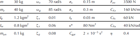
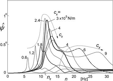
FIGURE 8.22 Steer vibration amplitude due to wheel unbalance as a function of wheel frequency of revolution n = Ω_o/2π for various values of the longitudinal suspension stiffness.

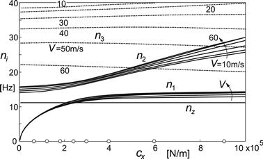
FIGURE 8.23 Variation of the three natural frequencies with longitudinal suspension stiffness at different speeds together with the constant vertical natural frequency. The circles on the horizontal axis mark the stiffness cases of Figure 8.22.

Clearly, in agreement with the variation of the natural frequencies assessed in this figure, the two resonance peaks move to higher frequencies when the stiffness is raised. A third resonance peak may show up belonging to the vertical natural frequency. This peak remains at the same frequency. It is of interest to observe that when the lowest steer natural frequency n₁ coincides with n_z the interaction between vertical and horizontal motions causes the peak to reach relatively high levels. As we have seen before, this interaction is brought about by the slope η indicated in Figure 8.13. The curves of the diagram of Figure 8.22 also exhibit the dip in the various curves that correspond with the zero’s (ω₀) of Figure 8.23. The zero frequency closely follows the formula (8.69) of the free system. At the lowest stiffness, the zero frequency n₀ almost coincides with the second natural frequency n₂ and suppresses the second peak.

It may be of interest to find out how the several tire parameters affect the response characteristics of Figure 8.22. In Figure 8.24 the result of making these parameters equal to zero has been depicted for the stiffness case c_x = 3 × 10⁵ N/m. Neglecting the factor η (case 1), meaning that the effective rolling radius would not change with load, appears to have a considerable effect indicating that, with η, the vertical motion does amplify the steering oscillation. Omitting the gyroscopic tire moment (2), while reinstating η, appears, as expected, to effectively decrease the steer damping. This is strengthened by additionally deleting the moment due to tread width (3). Omitting the relaxation lengths (4) lowers the peaks, thus removing the negative damping due to tire compliance. Deleting, in addition, the side force and the aligning torque (5) raises the peaks again, indicating that some energy is lost through the side slip. Disregarding the horizontal tire forces altogether (6) brings us back to the (horizontally) free system treated in the previous subsection. As predicted by the analysis, two sharp resonance peaks arise as well as the dip at the zero frequency.

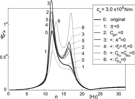
FIGURE 8.24 Influence of various tire parameters on the steer angle amplitude response curve.

8.5 ABS Braking on Undulated Road

The aim of this section is to investigate the influence of dynamic effects due to vertical and longitudinal wheel vibrations excited by road irregularities upon the braking performance of the tire and antilock braking system. These disturbing factors affect the angular velocity of the wheel and consequently may introduce disinformation in the signals transmitted to the ABS system upon which its proper functioning is based.

One may take the simple view that the primary function of the antilock device is to control the brake slip of the wheel to confine the wheel slip within a narrow range around the slip value at which the longitudinal tire force peaks. In the same range, it fortunately turns out that the lateral force that the tire develops as a response to the wheel slip angle is usually sufficient to keep the vehicle stable and steerable.

In order to keep the treatment simple, we will restrict the vehicle motion to straight-line braking and consider a quarter vehicle with wheel and axle that is suspended with respect to the vehicle body through a vertical and a longitudinal spring and damper. The analysis is based on the study of Van der Jagt et al. (1989).

8.5.1 In-Plane Model of Suspension and Wheel/Tire Assembly

The vehicle is assumed to move along a straight line with speed V. The forward acceleration of the vehicle body is considered to be proportional with the longitudinal tire force F_x. Vertical and horizontal vehicle body parasitic motions will be neglected with respect to those of the wheel axle. Consequently, the role of the wheel suspension is restricted to axle motion alone. These simplifications enable us to concentrate on the influence of the complex interactions between motions of the axle and the tire upon the braking performance of the tire. Figure 8.25 depicts the system to be studied. We have axle displacements x and z and a vertical road profile described by w and its slope dw/ds. To suit the limitations of the tire model employed, the wavelength λ of the road undulation is chosen relatively large. The wheel angular velocity is Ω and the braking torque is denoted with M_B. The unsprung mass and the polar moment of inertia of the wheel are lumped with a large part of those of the tire and are denoted with m and I_w.

FIGURE 8.25 System configuration for the study of controlled braking on undulated road surface.

Through the tire radial deflection the normal load is generated. Since we intend to consider possibly large slip forces, the analysis has to account for nonlinear tire characteristic properties. To adequately establish the fore and aft tire contact force, we will employ the enhanced transient tire model discussed in Section 7.3. The contact relaxation length σ_c will be disregarded here. In the model, a contact patch mass m_c is introduced that can move with respect to the wheel rim in tangential direction, thereby producing the longitudinal carcass deflection u. The contact patch mass may develop a slip speed with respect to the road denoted by . The transient slip is defined by (V > 0)

(8.85)

This longitudinal slip ratio is used as input in the steady-state longitudinal tire characteristic. The internal tire force that acts in the carcass and on the wheel axle will be designated as F_xa, while the tangential contact force is denoted with F_x. According to the theory, this slip force is governed by the steady-state force vs slip relationship F_x,ss(κ) which may be modeled with the Magic Formula. Since we have to consider the influence of a varying normal load, the relationship must contain the dependency on F_z. To handle this, the similarity method of Chapter 4 is used. We have the following equations:

(8.86)

with argument

(8.87)

The master characteristic F_x_o(κ) described by the Magic Formula holds at the reference load F_z_o which is taken equal to the average load. Its argument κ is replaced by the equivalent slip value κ_eq. Also, the longitudinal slip stiffness C_Fκ_o is defined at the reference load. In Figure 8.26, the steady-state force characteristics are presented for a set of vertical loads.

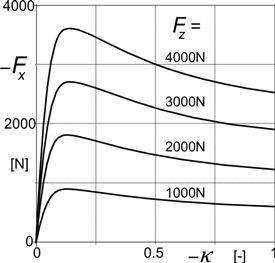
FIGURE 8.26 Steady-state tire brake force characteristics at different loads as computed with the aid of the Magic Formula and the similarity technique.

In-Plane Braking Dynamics Equations

The system has as input the road profile w and the brake torque M_B. The level w and the forward slope dw/ds are given as sinusoidal functions of the traveled distance s. To partly linearize the equations, the road forward slope is assumed to be small. The brake torque ultimately results from a control algorithm but may in the present analysis be considered as a given function of time.

The following equations apply for the wheel rotational dynamics, the horizontal and vertical axle motions, and the tangential motion of the contact patch mass:

(8.88)

(8.89)

(8.90)

(8.91)

with auxiliary equations for the tire loaded radius

(8.92)

the radial deflection

(8.93)

the effective rolling radius

(8.94)

the longitudinal carcass deflection rate

(8.95)

the wheel slip velocity

(8.96)

and the transient slip

(8.97)

Moreover, the following constitutive relations are to be accounted for

(8.98)

(8.99)

(8.100)

(8.101)

The function (8.101) is represented by Eqn (8.86) and illustrated in Figure 8.26. The remaining constitutive relations are simplified to linear expressions.

Frequency Response of Wheel Speed to Road Unevenness

As an essential element of the analysis we will assess the response of the wheel angular velocity variation to road undulations at a given constant brake torque. For this, the set of equations may be linearized around a given point of operation characterized by the average load F_z_o, the constant brake torque M_B_o, and the average slip ratio κ_o. We find for the constitutive relations,

(8.102)

(8.103)

(8.104)

(8.105)

where with the use of Eqns (8.86, 8.87)

(8.106)

and

(8.107)

For the variation in effective rolling radius, we have

(8.108)

The linearized equations of motion are obtained from the Eqns (8.88–8.91) by subtracting the average, steady-state values of the variable quantities, and neglect products of small variations.

The frequency response of Ω to w has been calculated for different values of the longitudinal suspension stiffness c_x. The average condition is given by the vehicle speed V_o = 60 km/h, a vertical load F_z_o = 3000 N, and a brake torque M_B_o = 300 Nm that corresponds to an average slip ratio κ_o = −0.021. The road undulation amplitude .

Some of the tire constitutive relations were determined directly from measurements while for some of the parameters values have been estimated. The small interaction parameters, η, e_xz, and e_zx, and also the rolling resistance parameters A_r and B_r have been disregarded. Table 8.3 lists the parameter values used in the computations.

TABLE 8.3 Parameter Values for Wheel/Tire/Suspension System

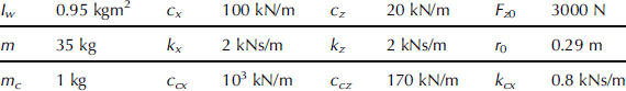
Figure 8.27 displays the amplitude of the wheel angular velocity variation as a function of the imposed frequency that is inversely proportional with the wavelength of the undulation. It is seen that the resonance peak height and the resonance frequency strongly depend on the fore and aft suspension stiffness.

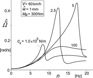
FIGURE 8.27 Frequency response of amplitude of wheel spin fluctuations to road undulations w at a constant speed V and brake torque M_B and for different values of the longitudinal suspension stiffness c_x.

8.5.2 Antilock Braking Algorithm and Simulation

The actual control algorithms of ABS devices marketed by manufacturers can be quite complex and are proprietary items which incorporate several practical considerations. However, almost all algorithms make use of raw data pertaining to the angular speed and acceleration of the wheels. A detailed discussion of the various algorithms for predicting wheel motions and modulating the brake torque accordingly has been given by Guntur (1975). The operational characteristic of a control algorithm used here for the purpose of illustration is shown in Figure 8.28. The salient features of the criteria used to increase or decrease applied brake torque (pressure) during a braking cycle depend critically upon both the momentary and threshold values of Ω and of . It is assumed that the brake torque rate can be controlled at three different levels. Upon application of the brake, the torque rises at a constant rate until point B is reached. After that, the torque is reduced linearly until point C. The brake torque remains constant in the interval between points C and E. Compound criteria are considered at points A and B for predicting when braking should be reduced to prevent the wheel from locking. Thus, we have from the starting of brake application

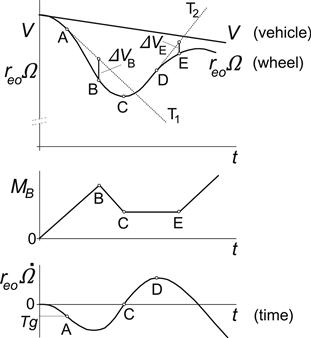
FIGURE 8.28 Example of an ABS algorithm used to modulate the applied brake torque.

Increase of torque for 0 < t < t_B according to dM_B/dt = R₁

The preliminary prediction time t_A is given by

where r_e_o stands for the nominal effective rolling radius and T for a nondimensional constant which sets the threshold for .

From time t_B we have

Decrease of torque for t_B < t < t_C according to dM_B/dt = R₂

The instant of prediction and action t_B is defined by

The time t_C marks the beginning of the constant torque phase CE, i.e.

Constant torque for t_C < t < t_E that is dM_B/dt = 0

Time t_C is found from

Similarly, the criterion for increasing the torque at E is:

Increase of torque for t > t_E according to dM_B/dt = R₁ is given by the compound reselection conditions generated at points D and E, with t_D and t_E being found from

and

For the simulation, the following values have been used:

T = −1, ΔV_B = 0.1r_e_o Ω (t_B) and ΔV_E = 1 m/s

The brake torque rates have been set to

In order to simulate the braking maneuver of a quarter vehicle equipped with the antilock braking system, the deceleration of the vehicle is taken to be proportional to F_x. The results of the simulations performed are presented in Figure 8.29. The left-hand diagrams refer to the case of braking on an ideally flat road, while the diagrams on the right-hand side depict the results obtained with the same system on a wavy road surface. For the purpose of simulation, the model was extended to include a hydraulic subsystem interposed between the brake pedal and the wheel cylinder. However, this extension is not essential to our discussion. In both cases, the same hydraulic subsystem was used and the same control algorithm as the one discussed above was implemented.

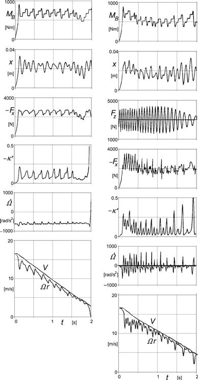
FIGURE 8.29 Left: Simulation of braking with ABS on an ideally flat road. Right: Simulation of braking with ABS on a wavy road.

The further parameters used in the simulation were

Initial speed of the vehicle: 60 km/h, the road input with a wavelength of 0.83 m and an amplitude of 0.005 m.

The results of the simulation show that brake slip variations occur both on a flat as well as on undulated road surfaces. However, the very large variations of the transient slip value in the latter case lead to a further deterioration of the braking performance. The average vehicle deceleration drops down from 7.1 m/s² to approximately 6 m/s².

Although large fluctuations in the vertical tire force are mainly responsible for this reduction, it is equally clear that severe perturbation occurring in both Ω and may be an additional source of misinformation for the antilock control algorithm. The important reduction in braking effectiveness resulting from vertical tire force variations may be attributed to the term C_cz in the linearized constitutive relation (8.106) of the rolling and slipping tire, and in particular to the contribution of the variation of the longitudinal slip stiffness with wheel load dC_Fκ/dF_z. Both vertical and horizontal vibrations of the axle and the vertical load fluctuations on wavy roads appear to adversely influence the braking performance of the tire as well as that of the antilock system.

In 1986, Tanguy made a preliminary study of such effects using a different control algorithm. He pointed out that wheel vibrations on uneven roads can pose serious problems of misinformation for the control logic of the antilock system. The results of the simulations discussed above and reported by Van der Jagt (1989) confirm Tanguy’s findings.

8.6 Starting from Standstill

In this section, the ability of the transient models to operate at and near-zero speed conditions will be demonstrated. The four models treated in Sections 7.2.2, 7.2.3, and 7.3 will be employed in the simulation of the longitudinal motion of a quarter vehicle model on an upward slope of 5%, cf. Figure 8.30.

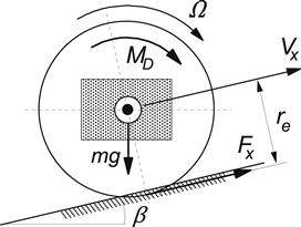
FIGURE 8.30 On the problem of starting from standstill on a slope.

The following three different maneuvers are considered:

• Standing still on slope, stepwise application of drive torque and subsequently rolling at constant speed.

• From standstill on slope, freely rolling backwards, then powerful propulsion followed by free rolling.

• From standstill, rolling backwards, then braking to wheel lock, followed by free rolling again after which a short phase of drive torque is applied. Finally, the quarter vehicle slows down on the slope.

The steady-state longitudinal force function of the transient longitudinal slip is described by the formula

(8.109)

For the successive transient tire models the equations will be repeated below.

Semi-non-linear transient model:

First-order differential equation for longitudinal tire deflection u according to Eqn (7.9):

(8.110)

where σ_κ only depends on a possibly varying vertical load F_z. The transient slip reads as

(8.111)

At low values of speed |V_x| < V_low the deflection u may have to be restricted as was formulated in general by Eqn (7.25). For our present problem, we have

if and |V_x| < V_low and (V_sx + |V_x|u/σ_κ)u < 0:

(8.112)

else

(8.113)

The slip where the peak force occurs is roughly

(8.114)

with the slip stiffness

(8.115)

For the factor A the value 1 is suggested but a higher value may improve the performance, especially when the force characteristic exhibits a pronounced peak.

Fully nonlinear transient model:

The same Eqns (8.110, 8.111) hold but with σ_κ replaced by the -dependent and downwards limited quantity:

(8.116)

where σ_κ_o represents the value of the relaxation length at . We have the equation

(8.117)

The transient slip now reads as

(8.118)

A deflection limitation is not necessary for this model. However, because of the algebraic loop that arises, the quantity (8.116) must be obtained from the previous time step.

Restricted fully nonlinear model:

Analogous to Eqn (7.35) we have the equation for

(8.119)

with the -dependent relaxation length

(8.120)

The model is not sensitive to wheel load variations which constitutes the restriction of the model. For the problem at hand, this restriction is not relevant and the model can be used. The great advantage of the model is the fact that an algebraic loop does not occur, and again, a u limitation is not needed. A straightforward simulation can be conducted. For the relation (8.120) the following approximate function is used:

(8.121)

where σ_min represents the minimum value of the relaxation length that is introduced to avoid numerical difficulties.

Enhanced nonlinear transient model:

Following Section 7.3 and Figure 7.15, we have for the differential equation for the longitudinal motion of the contact patch mass m_c

(8.122)

where F_x denotes the contact force governed by Eqn (8.109).

The transient slip value is obtained from the differential Eqn (7.56)

(8.123)

an equation similar to (8.119) but here with a constant (small) contact relaxation length. The longitudinal carcass stiffness c_cx in the contact zone should be found by satisfying the equation

(8.124)

The deflection rate needed in Eqn (8.122) is equal to the difference in slip velocities of contact patch and wheel rim:

(8.125)

The longitudinal force acting on the wheel rim results from

(8.126)

Low-speed additional damping:

At zero forward speed with each of the first three tire models, a virtually undamped vibration is expected to occur. An artificial damping may be introduced at low speed by replacing in (8.109) by

(8.127)

which corresponds with the suggested Eqn (7.26). The gradual reduction to zero at V_x = V_low is realized by using the formula

(8.128)

Also with the enhanced model, the additional damping will be introduced while k_cx is taken equal to zero to better compare the results.

Vehicle and wheel motion:

For the above tire models, the wheel slip speed follows from

(8.129)

The vehicle velocity and the wheel speed of revolution are governed by the differential equations:

(8.130)

(8.131)

where r_e is the effective moment arm which turns out to correspond with experimental evidence, cf. Chap. 9, Figure 9.34. For the first three models with contact patch mass not considered, we have

(8.132)

When at braking the wheel becomes locked, we have Ω = 0.

Results:

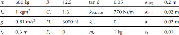
The three different longitudinal maneuvers listed above have been simulated with each of the four transient tire models. In Figures 8.31–8.34, some of the results are presented. The parameter values are listed in Table 8.4.

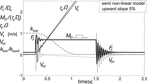
FIGURE 8.31 Standing still on slope, acceleration, and subsequently rolling at constant speed. Tire/wheel wind-up oscillations occur both at start and at end of step change in propulsion torque M_D. Computations have been performed with the semi-non-linear transient tire model with constant relaxation length (V_low = 2.5 m/s).

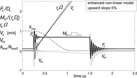
FIGURE 8.32 Same simulation as in Figure 8.31 but now using the enhanced nonlinear transient tire model with carcass compliance (V_low = 2.5 m/s). Only at low speed a frequency difference can be observed to occur. Very similar results are obtained with the fully nonlinear transient models with changing relaxation length.

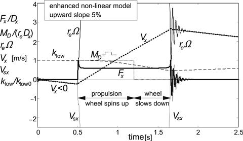
FIGURE 8.33 From standstill on slope, freely rolling backward, then powerful propulsion followed by free rolling. The tire longitudinal force passes its peak and reaches the lower end of its characteristic which enables the wheel to spin up. Next, when the wheel slows down rapidly, the peak is reached again and a damped wheel/tire wind-up oscillation occurs. Calculations using enhanced transient tire model (V_low = 5 m/s). Together with the restricted fully nonlinear model, the enhanced model turns out to perform best.

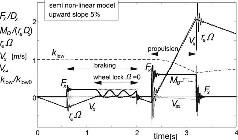
FIGURE 8.34 From standstill rolling backward, then braking to wheel lock, followed by free rolling again after which a short phase of acceleration occurs. Finally, the quarter vehicle slows down on the slope. During wheel lock, the vehicle vibrates at low frequency with respect to the ‘contact patch’. Calculations with the simple semi-non-linear transient tire model. Practically the same results are obtained when using one of the other three transient tire models.

TABLE 8.4 Parameter Values

Figures 8.31 and 8.32 depict the process of standing still on a 5% upward slope (appropriate brake or drive torque), followed by a step drive torque input and subsequently rolling at constant speed (back to equilibrium drive torque). Tire/wheel wind-up oscillations occur both at start and at end of step change in propulsion torque M_D. Results have been shown of the computations using the semi-non-linear transient tire model (Figure 8.31) and the enhanced model (Figure 8.32). Virtually the same results as depicted in Figure 8.32 have been achieved by using either the fully nonlinear or the restricted nonlinear transient tire model. Only at low speed, a frequency difference can be observed to occur when using the semi-non-linear model.

Figure 8.33 shows the results of standing on the slope, then freely rolling backward, subsequently applying powerful propulsion, which is followed by free rolling. The tire longitudinal force passes its peak and reaches the lower end of its characteristic, which enables the wheel to spin up. Next, when the wheel slows down rapidly, the peak is passed again and a damped wheel/tire wind-up oscillation occurs. Calculations have been performed using the enhanced transient tire model of Section 7.3 (with contact mass). The restricted fully nonlinear tire model, Eqn (7.35) not responding to load changes, turns out to yield almost equal results. The other two models, especially the semi-non-linear model of Section 7.2.3 (with σ constant), appear to perform less good under these demanding conditions (less F_x reduction in spin-up phase which avoids an equally rapid spinning up of the wheel). The low-speed limit value V_low was increased to 5 m/s to restrict the u deflection of the semi-non-linear model over a larger speed range. The factor A was increased to 4 which improved the performance of this model. Omission of the limitation of the u deflection would lead to violent back and forth oscillations.

Finally, Figure 8.34 depicts the simulated maneuver: from standstill rolling backwards then braking to wheel lock, which is followed by free rolling again after which a short phase of acceleration occurs; finally, the quarter vehicle slows down on the slope. During wheel lock the vehicle mass appears to vibrate longitudinally at low frequency with respect to the ‘contact patch’. Calculations have been conducted with the simple semi-non-linear transient tire model. Practically equal results have been obtained when using one of the other three transient tire models.

It may be concluded that the restricted fully nonlinear model and the enhanced model with contact patch mass show excellent performance. It should be kept in mind that the restricted model does not react on wheel load variations. The semi-non-linear model can be successfully used under less demanding conditions.

The next chapter deals with the development of a more versatile tire model which can handle higher frequencies and shorter wavelengths. The enhanced model and the restricted fully nonlinear transient tire model will be used as the basis of this development.

..................Content has been hidden....................

You can't read the all page of ebook, please click here login for view all page.

Table of Contents for Chapter 8. Applications of Transient Tire Models

Create new playlist

Sign In

Sign Up

Chapter 8

Applications of Transient Tire Models

Chapter Outline