
Chapter 9
Short Wavelength Intermediate Frequency Tire Model
Chapter Outline
9.2. The Contact Patch Slip Model
9.2.1. Brush Model Non-Steady-State Behavior
9.2.2. The Model Adapted to the Use of the Magic Formula
Steady-State, Step Response, and Frequency Response Characteristics
9.1 Introduction
In Chapter 5 the stretched string model, possibly featuring tread elements and tire inertia (gyroscopic couple), was used to study the dynamic response of the side force and aligning torque to lateral, vertical, and yaw motion variations of the wheel axle. These motions, however, had to be restricted in magnitude to allow the theory to remain linear. Several approximations were introduced to simplify the model description, which made it possible to consider ranges of relatively large slip through a simple nonlinear extension. The limitation of the use of this type of simplified models is that only phenomena with relatively large wavelength (>ca. 1.5 m) and low frequency (<ca. 8 Hz) can be approximately handled.
The present chapter describes a model that is able to cover situations where the wavelength is relatively short (>ca. 10 cm and even shorter for modeling road obstacle enveloping properties) and the frequency is relatively high (<ca. 80 Hz) while the level of slip can be high. Situations in which combined slip occurs can be handled and the Magic Formula model can be used as the basis for the nonlinear force and moment description. As a result, a continuous transition from time-varying slip situations to steady-state conditions is realized. The original model development was restricted to the more important responses to variations of longitudinal and side slip. Also, the possibility to traverse distinct road irregularities (cleats) was included in the tire model. The model is based on the work of Zegelaar (1998) and Maurice (2000) conducted at the Delft University of Technology and supported by TNO Automotive and a consortium of industries. The model is referred to as the SWIFT model (corresponding to the title of the present chapter). Subsequent developments of the model made it possible to also include variations of camber and turn slip.
The crucial step that was taken to reach further than one can by using the string model is the separation of modeling the carcass and the contact patch. In this way a much more versatile model can be established that correctly describes slip properties at short wavelengths and at high levels of slip. The model achieved can be seen as a further development of the enhanced single contact point model of Section 7.3, Figure 7.15.
Five elements of the model structure can be distinguished: (1) The inertia of the belt that has been taken into account to properly describe the dynamics of the tire. The restriction to frequencies of about 60 Hz allows the belt to be considered as a rigid circular ring. (2) The so-called residual stiffnesses, see explanation below, that have been introduced between contact patch and ring to ensure that the total static tire stiffnesses in vertical, longitudinal, lateral, and yaw directions are correct. The total tire model compliance is made up of the carcass compliance, the residual compliance (in reality a part of the total carcass compliance), and the tread compliance. (3) The brush model that represents the contact patch featuring horizontal tread element compliance and partial sliding. On the basis of this model, the effects of the finite length and width of the footprint are approximately included. This element of the model is the most complex part and accomplishes the reduction of the allowed input wavelength to ca. 10 cm. (4) Effective road inputs to enable the simulation of the tire moving over an uneven road surface with the enveloping behavior of the tire properly represented (Chapter 10). The actual three-dimensional profile of the road is replaced by a set of four effective inputs: the effective height, the effective forward and transverse slopes of the road plane, and the effective forward road curvature that is largely responsible for the variation of the tire effective rolling radius. (5) The Magic Formula tire model to describe the nonlinear slip force and moment properties. In Figure 9.1 the model structure has been depicted.
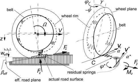
FIGURE 9.1 General configuration of the SWIFT model featuring rigid belt ring, residual stiffnesses, contact patch slip model, and effective road inputs.
Similar more physically oriented models have been developed. A notable example is the BRIT model of Gipser. He employs a brush-ring model featuring tread elements distributed over a finite contact patch with realistic pressure distributions and demonstrates the use of the model with simulations of the tire traversing a sinusoidal road surface also at a slip angle and at braking, cf. Gipser et al. (1997). Other models: FTire and RMOD-K, have been developed by Gipser (cf. Section 13.2) and Oertel and Fandre (cf. Section 13.1), respectively. In Chapter 13 outlines of these two models and of the SWIFT model are presented.
In the ensuing theoretical treatment, firstly, in Section 9.2, the slip model of the contact patch covering small wavelengths and large slip will be dealt with. Secondly, the model for the description of the dynamic behavior of the rigid belt ring will be added, Section 9.3. Thirdly, the feature of the model that takes care of running over uneven roads will be addressed, cf. Chapter 10. Full-scale tire test results demonstrate the validity of the model.
9.2 The Contact Patch Slip Model
In this section, we will first represent the contact patch with tread elements by the brush model. Because of its relative complexity, the analytical model that describes the non-steady-state response to slip variations is approximated by a set of first-order differential equations. This contact model is tested by attaching the base line of the brush model to the wheel plane through a compliant carcass. For reasons of practical use, we finally introduce the Magic Formula to handle realistic nonlinear slip behavior of the model.
9.2.1 Brush Model Non-Steady-State Behavior
The steady-state characteristics of the brush model have been discussed in Chapter 3. As a first step, we will derive the equations that govern the response of the forces and moment to small variations of the wheel slip with respect to a given level of wheel slip indicated with subscript o.
Longitudinal Slip
For the case of pure longitudinal slip κcoof the contact patch, the point of transition from adhesion to sliding is located according to Eqn (3.44) with (3.34, 3.40) at a distance xt from the contact center:
![]() (9.1)
(9.1)
The composite parameter θ has been defined in Chapter 3, Eqn (3.46). The length of the adhesion range 2am = a − xt that begins at the leading edge is characterized by the fraction m that in the present chapter replaces the symbol λ to avoid confusion with the notation for the wavelength. We have
![]() (9.2)
(9.2)
An important observation is that at small variations of slip we may assume that only in the adhesion range changes in deflection occur.
For the development of the transient model we start out from the basic rolling contact differential Eqns (2.55, 2.56). In the adhesion range we find for the longitudinal tread element deflection uc in the case that only longitudinal slip is considered:
![]() (9.3)
(9.3)
where the tilde designates the variation with respect to the steady-state level. The average linear speed of rolling of the contact patch is equal to that of the wheel rim and reads
![]() (9.4)
(9.4)
The Fourier transform of the deflection becomes with U and K denoting the transformed quantities of u and κ, respectively, and ωs the path frequency:
![]() (9.5)
(9.5)
Here, the boundary condition that says that the deflection vanishes at the leading edge, is satisfied. By integrating over the range of adhesion and multiplying with the tread element stiffness cp, the frequency response function of the variation of Fx to the variation of κc is obtained. With the reduced frequency
![]() (9.6)
(9.6)
and the local derivative of Fx to κc
![]() (9.7)
(9.7)
the expression for the response function becomes, when still adhesion occurs in the contact patch (first condition of (9.2)),
![]() (9.8)
(9.8)
In Figure 9.2 the resulting amplitude and phase characteristics have been shown together with those of an approximate first-order system. Especially the phase curve appears to exhibit a wavy pattern in the higher frequency range. These waves are considerably attenuated when the contact model is incorporated in a more complete tire model including carcass compliance, as will be shown below.
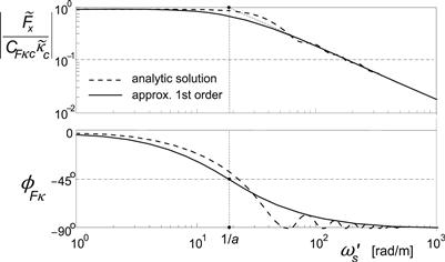
FIGURE 9.2 Frequency response function of the longitudinal force variation to longitudinal slip variation of the brush model versus reduced path frequency according to the exact analytical solution and that of an approximate substitute first-order system at a given level of longitudinal slip.
The first-order substitute model has a frequency response function that reads
![]() (9.9)
(9.9)
The approximation shows the same high frequency asymptote and steady-state level as the exact model. Apparently, the actual cutoff path frequency reads
![]() (9.10)
(9.10)
that, obviously, reduces to 1/a when the average slip κco vanishes and, as a consequence, m (9.2) becomes equal to unity. When the average slip is chosen larger, the length of the adhesion range decreases and the cutoff frequency becomes higher. The relaxation length of the approximate contact model reads, according to Eqn (9.9) with (9.6),
![]() (9.11)
(9.11)
which reduces to zero when total sliding occurs.
The performance of the first-order system is reasonable but appears to improve when the filtering action of the carcass compliance is taken into account. In that configuration, we have the wheel slip velocity Vsx that acts as the input quantity. Adding the time rate of change of the carcass deflection produces the slip velocity of the brush model. The carcass deflection u equals (with fore-and-aft carcass stiffness cx introduced)
![]() (9.12)
(9.12)
The feedback loop in the augmented system apparently contains a gain equal to iωs/cx. The resulting complete frequency response function reads
![]() (9.13)
(9.13)
When the approximate first-order system is employed for the contact model, the frequency response function for the complete model becomes, using (9.13) with (9.9),
![]() (9.14)
(9.14)
where the total relaxation length has been introduced which apparently reads
![]() (9.15)
(9.15)
The local longitudinal slip stiffness of the contact patch is here equal to the local longitudinal slip stiffness of the complete model, which obviously is due to the assumed inextensibility of the base line of the brush model. So we have at steady state:
![]() (9.16)
(9.16)
At vanishing slip we will add a subscript 0. When total sliding occurs, both σc and CFκ reduce to zero and the total relaxation length σ vanishes.
Introduction of the longitudinal carcass compliance may be accomplished by considering the feedback loop similar to the one (cy) for the more complex configuration for lateral slip shown in Figure 9.6. Figure 9.3 presents the frequency response function for this total model at vanishing slip, κ0 = 0.
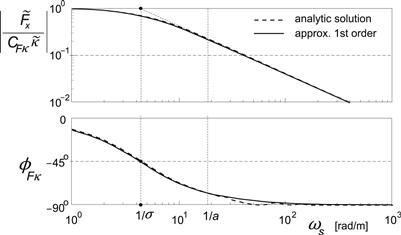
FIGURE 9.3 Frequency response function of the longitudinal force variation to longitudinal slip variation of the brush model attached to a flexible carcass versus path frequency according to the exact analytical solution and that of the approximate first-order system at zero longitudinal slip.
It is noted that compared with the curves of Figure 9.2 the wavy pattern is considerably reduced. The approximate system performs very well. A wavelength of 10 cm occurs at the path frequency ωs = ca. 60 rad/m.
The differential equation that governs the transient slip response of the contact patch and through that the longitudinal force response becomes for the approximate system
![]() (9.17)
(9.17)
The variation of the force becomes
![]() (9.18)
(9.18)
The structure of Eqn (9.17) corresponds with that of Eqn (7.37) of Chapter 7. The response, however, is insensitive to load variations but shows a nice behavior. The transient response to load variations is sufficiently taken care of through the effect of carcass compliance. As a result, the relaxation length for the response to load variations becomes equal to CFκc/cx, which is somewhat smaller than σ (9.15) that holds for the response to slip variations.
When the average steady-state relation for the longitudinal slip
![]() (9.19)
(9.19)
is added to Eqn (9.17), the equation for the total transient slip is obtained:
![]() (9.20)
(9.20)
that completely corresponds to Eqn (7.54) of the enhanced nonlinear transient tire model. The transient slip ![]() is subsequently used as input into the steady-state longitudinal force characteristic, as will be explained later on, and has already been indicated in Chapter 7, Section 7.3.
is subsequently used as input into the steady-state longitudinal force characteristic, as will be explained later on, and has already been indicated in Chapter 7, Section 7.3.
Lateral Slip
The lateral slip condition is more complex to handle because we have to deal with both the side force and the aligning torque. In addition, in the test condition, the carcass is allowed to not only deflect in the lateral direction but also about the vertical axis. This is in accordance with the ultimate SWIFT configuration. The connected turn slip behavior of the contact patch will be dealt with further on.
As with the longitudinal model development, first, the analytic response functions of the brush model will be assessed, in this case to side slip variations. Eqn (2.56) gives rise to the following equation for the lateral tread deflection variations:
![]() (9.21)
(9.21)
Note that for the sake of simplification in the present chapter the notation tanα is replaced by α, with or without a subscript. As for the longitudinal deflection we find for the Fourier transform Vc of the lateral deflection responding to slip angle variations, Ac denoting the brush model slip angle’s transform (or actually of tan αc):
![]() (9.22)
(9.22)
Again, the responses to variations of the side slip only occur in the range of adhesion. The transition point from adhesion to sliding now occurs at
![]() (9.23)
(9.23)
and the corresponding adhesion fraction becomes, cf. Eqn (3.8),
![]() (9.24)
(9.24)
As the slip angle of the contact patch remains small in the range where adhesion still occurs, cos αco has been replaced by unity. By integration of the transformed deflection over the range of adhesion the frequency response functions of the force and the moment variations are established. They read, at pure lateral slip (Vrco = Vx, cf. (9.4)),
![]() (9.25)
(9.25)
and
![]() (9.26)
(9.26)
The local slope of the steady-state side force characteristic of the brush model is given by
![]() (9.27)
(9.27)
The normalized response function of the side force is identical to that of the longitudinal force if the factor 1 + κco is omitted in (9.6). The approximate first-order description with response function
![]() (9.28)
(9.28)
where
![]() (9.29)
(9.29)
shows the same very good agreement with the exact result, as assessed with the longitudinal force response. Similarly we have the differential equation for the variation of the transient side slip:
![]() (9.30)
(9.30)
The variation of the side force becomes
![]() (9.31)
(9.31)
After adding the steady-state equation
![]() (9.32)
(9.32)
to Eqn (9.30), the equation for the total transient side slip is obtained:
![]() (9.33)
(9.33)
As before, the resulting ![]() is used as the input of the steady-state side force function.
is used as the input of the steady-state side force function.
We may follow the same procedure to assess the aligning torque equations as was done in Section 7.3. The resulting first-order response, however, does not always agree with the analytically found tendency. The phase lag and the slope of the high-frequency amplitude asymptote indicate that a second-order behavior prevails at zero average slip angle while at larger slip angles the response gradually changes into a first-order nature. Apparently, the mechanism is more complex and we should account for the transient response of the pneumatic trail. The variation of the aligning torque may be written as follows:
![]() (9.34)
(9.34)
The analysis conducted by Maurice (2000) shows that the analytically assessed response function of the pneumatic trail variation to slip angle variations can be approximated by the first-order system (9.33) and a so-called phase leading network in series. The frequency response function of the latter reads
![]() (9.35)
(9.35)
The factor in this formula represents the local slope of pneumatic trail characteristic:
![]() (9.36)
(9.36)
which, apparently, is a negative quantity. According to Maurice, adequate values for the parameters σ1 and σ2 can be obtained through the formulas
![]() (9.37)
(9.37)
or alternatively
![]() (9.38)
(9.38)
and
![]() (9.39)
(9.39)
The block diagram of the current system governed by Eqns (9.28, 9.34, 9.35) is presented in the upper diagram of Figure 9.4. The lower diagram shows an alternative structure of the same system, thereby displaying the extra moment ΔMz, which is governed by the ratio of parameters (9.39). This ratio tends to infinity when full adhesion occurs. Then, m = 1 and αco = 0, as becomes clear from Eqn (9.24). The singularity involved has been circumvented by Maurice through the introduction of a function that limits the value of (9.39) around zero lateral slip, αco = 0. This, however, will slightly disturb the proper response at zero slip angle and thus degrades the linear analysis around zero slip. An alternative way of avoiding the singularity, which obviously is caused by the fact that we actually may have a moment without the simultaneous presence of a force, is the consideration of the extra transient moment ΔMz. This moment is obtained by multiplication of the difference of the transient slip quantities for the force and for the pneumatic trail with three factors the combination of which may be designated with CΔM:
![]() (9.40)
(9.40)
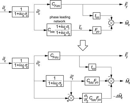
FIGURE 9.4 Block diagram of the contact patch model to generate short wavelength transient responses of the side force and the aligning torque to small slip angle variations. The original upper diagram can be replaced by the lower diagram, thereby avoiding singularity at zero slip.
It turns out that now the singularity does not show up because both Fyo and 1/σ1 become zero at the same time. This indicates that indeed a moment may arise although at that instant of time the side force is zero. After writing out the factors in (9.40) by using expressions for the side force (3.11), the pneumatic trail (3.13) and further (9.36, 9.39) while in (3.11) λ is replaced by m and θyσy by θαco = z we find, for CΔM,
![]() (9.41)
(9.41)
where CMαco denotes the aligning stiffness of the brush model at zero slip angle and the nondimensional factor ξ; is introduced:
![]() (9.42)
(9.42)
with
![]() (9.43)
(9.43)
Evaluation of (9.42) reveals that for z < 1 the factor ξ; may possibly be approximated by
![]() (9.44)
(9.44)
This approximation will be introduced later on when we will deal with the application of the Magic Formula.
The differential equations that apply for the contact patch model subjected to small side slip variations with respect to a given side slip level now read
![]() (9.45)
(9.45)
![]() (9.46)
(9.46)
from which the variation of the force and moment result:
![]() (9.47)
(9.47)
![]() (9.48)
(9.48)
It is of importance to check the step responses to side slip starting from zero slip angle, especially right after the start of the step change. Initially we have all variables equal to zero while the slip angle input has reached the new value αco. The various time derivatives become
 (9.49)
These results are correct. The last equation holds indeed because we have at vanishing slip angle according to Eqn (9.42): ξ; = 1 and consequently CΔM = tcoCFαco, where tco = a/3. Evidently, the extra moment is responsible for the proper start of the course of the aligning torque showing zero slope. This property has been ascertained to occur both in reality and with models, cf. Figures 5.10 and 5.11. Also the response to a lateral wheel displacement y = ∫Vsydt at zero forward speed develops correctly. We find with Eqn (7.6) for the force: Fy = −CFy y and for the moment: Mz = 0.
The equations may now further be appraised by first introducing tire carcass lateral and torsional compliance, as depicted in Figure 9.5 and in the corresponding block diagram of Figure 9.6, and subsequently comparing the results with analytical solutions obtained by using Eqns (9.25, 9.26).
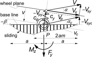
FIGURE 9.5 The brush model attached to a carcass possessing lateral and torsional compliance.
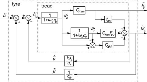
FIGURE 9.6 Block diagram of the augmented system including carcass lateral and torsional compliance.
As a reference, the steady-state characteristics of the model have been presented in Figure 9.7. The diagram contains the curves for both the complete model and for the brush model alone. It is of interest to note the lower cornering stiffness due to the introduction of carcass compliance. The expression for the lower side slip stiffness can be found to read
![]() (9.50)
(9.50)
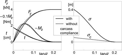
FIGURE 9.7 Steady-state side slip force and moment characteristics and the relaxation length of the brush model (the contact patch) and of the model including the flexible carcass through which the brush model is attached to the wheel plane.
The relaxation length of the complete model found from the cutoff frequency of the side force response function turns out to become
![]() (9.51)
(9.51)
The way the relaxation length changes with slip angle is depicted in the right-hand diagram of Figure 9.7. As one might expect, we find that this length multiplied by the increment in wheel slip angle is equal to the increase of the sum of carcass lateral deflection and the average deflection of the adhering tread elements.
At three different levels of side slip, αo = 0, 0.08, and 0.16 rad, the comparison of the simulation model with the analytical model has been conducted in terms of the path frequency response functions. Figure 9.8 shows the results. The general conclusion is that, at least for wavelengths larger than ca. 15 cm, the correspondence can be judged to be very good. The upper pair of diagrams that refer to the side force response shows the sideways ‘shift’ of the phase lag curves that is caused by the drop in relaxation length with increasing average slip angle. The diagram for the aligning torque response clearly shows the transition from second- to first-order behavior when the average slip angle changes from zero to larger values.
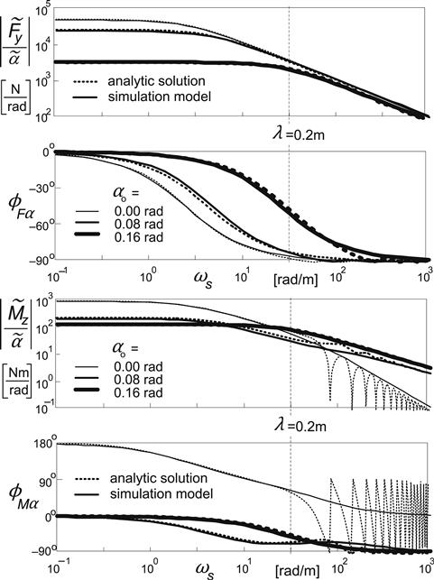
FIGURE 9.8 Frequency response functions of a linearized system including carcass flexibility at different average slip angle levels according to the analytical solution and to the approximate simulation model. The path frequency at a wavelength of the input wheel plane motion equal to 20 cm has been indicated.
The Eqns (9.45–9.48) can be made applicable to the general case of large slip angle variations by adding to (9.45, 9.46) the steady-state relations and by rewriting the Eqns (9.47, 9.48) in complete nonlinear form so that, when considering a small variation, the linearized equations are recovered. We obtain, for the transient slip quantities,
![]() (9.52)
(9.52)
![]() (9.53)
(9.53)
and, for the force and moment,
![]() (9.54)
(9.54)
![]() (9.55)
(9.55)
The last term representing the extra moment is left in linearized form. This term may be replaced by the difference of two equal functions the derivative of which equals CΔM, one with argument ![]() and the other with
and the other with ![]() . Because of the fact that the difference of these two arguments remains small, the linearized version is expected to be sufficiently accurate. The block diagram of the nonlinear system displayed in Figure 9.9 may further clarify the structure of the model.
. Because of the fact that the difference of these two arguments remains small, the linearized version is expected to be sufficiently accurate. The block diagram of the nonlinear system displayed in Figure 9.9 may further clarify the structure of the model.
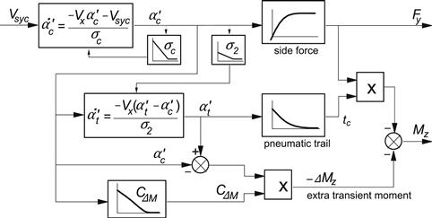
FIGURE 9.9 Block diagram of the nonlinear model of the contact patch (tread) also valid for larger slip angle variations.
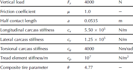
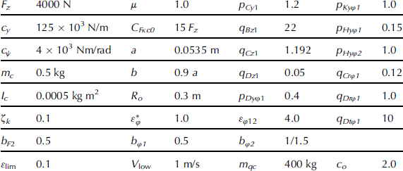
To ensure that the above equations correctly describe the response to large slip angle variations, the simulation model results have been compared with the response of a physical model. That model features a finite number of tread elements attached to a straight base line. The deflections of carcass and elements are computed at each time step in which the wheel is rolled further over a distance equal to the interval between two successive tread elements and is moved sideways according to the current value of the input slip angle. The actual model employed contains 20 elements. The parameter values used in both models have been listed in Table 9.1.
TABLE 9.1 Parameter Values Used for Brush Model with Flexible Carcass
The slip angle variation is sinusoidal around a given average level. To cover a broad range of operations, the computations have been conducted at three wavelengths: λ = 0.2, 1, and 5 m, two average slip angle levels: αo = 0 and 0.08 rad, and one amplitude: ![]() .
.
Figure 9.10 presents the results for the two models. The range of the abscissa has been chosen such that precisely two wavelengths are covered. The distance rolled is large enough to have a situation close to the periodic state. Again, the agreement is quite good and we may have confidence in the model. The bottom diagram presents the variation of the slip angle. The top pair of diagrams shows the responses at the relatively long wavelength of 5 m so that a condition closer to steady state has been reached. From Figure 9.7 it can be seen that at the maximum α of 0.16 rad or almost 9° the aligning torque peak has been surpassed by far. This explains the two dips per wavelength. At a maximum of 0.08 rad the peak has just been surpassed.
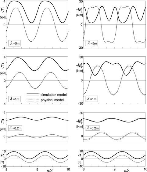
FIGURE 9.10 Side force and aligning torque responses of the nonlinear brush simulation model with flexible carcass to sinusoidal slip angle input of the wheel plane with a slip angle amplitude of 0.08 rad and average levels of 0 (thin curves) and 0.08 rad (fat curves), compared with results of the physical model (broken curves).
The less deep dips occurring in the upper curves of diagrams b and d are delayed with respect to the slip angle when this has reached its minimum value equal to zero. At steady state, when λ → ∞, the moment (and the force) would have become equal to zero at that instant. The deeper dips belong to the maxima of the slip angle variation. The considerable reduction in amplitude of the response at the shorter wavelengths agrees nicely with the findings of Figure 9.8.
The force responses correspond almost perfectly with the outcome of the physical model. Evidently, a similar correspondence is expected to occur with the response of the longitudinal force to longitudinal slip variations.
Turn Slip
The last item to be studied in the development of the contact model is the response to variations in path curvature while the slip angle remains zero. We will not attempt to develop a background analytical model but will take a more heuristic route. The results will be checked by comparing these with the computed responses of the physical model. The responses derived for the string model with tread elements as presented in Chapter 5, especially the step responses to φ as depicted in Figure 5.21 (ex.tr.el.) and Figure 5.10 may be helpful. We observe that the force response is similar to that of the aligning torque to a step change in slip angle. In both cases the slope at the start is zero.
The side force relates to the transient turn slip (if linear) as: ![]() . The uncorrected further approach of the force to its steady-state level is assumed to occur according to the first-order equation, with σc as relaxation length. The initial slope of the uncorrected response curve of the normalized transient turn slip of the contact patch
. The uncorrected further approach of the force to its steady-state level is assumed to occur according to the first-order equation, with σc as relaxation length. The initial slope of the uncorrected response curve of the normalized transient turn slip of the contact patch ![]() versus s becomes: 1/σc. The zero slope at the start may be modeled by subtracting a correction response curve that starts with the same slope but dies out after having reached its peak. Such a short term response may be obtained by taking the difference of two responses,
versus s becomes: 1/σc. The zero slope at the start may be modeled by subtracting a correction response curve that starts with the same slope but dies out after having reached its peak. Such a short term response may be obtained by taking the difference of two responses, ![]() , each leading to the same level but starting at different slopes the difference of which should correspond to the initial slope of the uncorrected force response curve. For simplicity we take for one of the two responses
, each leading to the same level but starting at different slopes the difference of which should correspond to the initial slope of the uncorrected force response curve. For simplicity we take for one of the two responses ![]() the uncorrected force response, so that σF1 = σc. The relaxation length of the second response
the uncorrected force response, so that σF1 = σc. The relaxation length of the second response ![]() should then be equal to σF2 = σc/2, so that its initial slope becomes: 2/σc. Subtracting these two slopes results in the desired initial slope of the correction curve: 1/σc. The resulting equations for the force response to the turn slip velocity
should then be equal to σF2 = σc/2, so that its initial slope becomes: 2/σc. Subtracting these two slopes results in the desired initial slope of the correction curve: 1/σc. The resulting equations for the force response to the turn slip velocity ![]() read
read
![]() (9.56)
(9.56)
![]() (9.57)
(9.57)
with σF2 = σc/2. The transient turn slip for the force finally becomes
![]() (9.58)
(9.58)
The side force at pure path curvature is obtained from the nonlinear steady-state response function:
![]() (9.59)
(9.59)
For the range of turn slip a|φ| < 1/θ the relation remains linear and equals for the brush model:
![]() (9.60)
(9.60)
The moment response may be divided into the response due to the contact patch length that involves lateral tread deflections, and the response due to tread width giving rise to longitudinal deflections. First, we will address the moment generated by the brush model with zero width. Figures 5.9, 5.10, and 5.21 indicate that we are dealing here with a response that after having reached a peak tends to zero. Again we may model this behavior by subtracting two first-order responses. For this, we introduce two transient turn slip quantities ![]() and
and ![]() with respective relaxation lengths: σφ1 and σφ2. The two differential equations become
with respective relaxation lengths: σφ1 and σφ2. The two differential equations become
![]() (9.61)
(9.61)
![]() (9.62)
(9.62)
At zero speed the response of the difference would become
![]() (9.63)
(9.63)
The deflection angle of the tread due to transient spin is defined as
![]() (9.64)
(9.64)
![]() (9.65)
(9.65)
The condition to be satisfied is that the deflection angle is equal to the yaw angle: ![]() . Hence, we have
. Hence, we have
![]() (9.66)
(9.66)
In the case of small angles, we may write for the moment
![]() (9.67)
(9.67)
From Eqns (9.61 and 9.62), it can be assessed that the initial slope of the response of the moment to a step change in spin ![]() from zero to φc0 turns out to be
from zero to φc0 turns out to be
![]() (9.68)
(9.68)
For the second condition to assess the ratios of the σφ’s to half the contact length a, the best fit of the remaining course of the step response may serve, cf. Eqns (9.114 and 9.115).
When the angle of rotation ψ continues to grow, the state of total sliding will be attained and the moment can be calculated to become
![]() (9.69)
(9.69)
It has not been tried to derive the functional relationship between moment and increasing steer angle for the standing (nonrolling) brush model. The following nonlinear function to describe the moment response in between the two extremes has been chosen:
![]() (9.70)
(9.70)
The factor εφ has been introduced to have a parameter available to better approach the response shown by the physical model. The value 1.15 appeared to be appropriate. Similar to the relaxation length σc, Eqns (9.29 and 9.24), the lengths σφ1,2 are reduced in proportion with the magnitudes of transient turn slip quantities ![]() and
and ![]() .
.
For the evaluation of the model a comparison with the physical brush model has been executed. First, the flexible carcass is attached to the tread model, cf. Figure 9.5. To simulate this more complex situation, the approach of the enhanced transient model of Section 7.3 has been adopted. The additional dynamic equations for the contact patch with mass mc and moment of inertia Ic and carcass stiffnesses cy,ψ and damping coefficients ky,ψ read, cf. Figure 9.5:
![]() (9.71)
(9.71)
![]() (9.72)
(9.72)
![]() (9.73)
(9.73)
![]() (9.74)
(9.74)
![]() (9.75)
(9.75)
This extension of the model may, of course, also be used for the previously treated response to pure side slip. In fact, it is to be noted that the model for side slip, Eqns (9.52–9.55), should be added to the spin model, Eqns (9.61, 9.62, 9.64, and 9.70), to correctly account for their interaction in the complete model with carcass compliance included. In the physical model the brush model automatically responds to both the side slip and spin. When the wheel plane is subjected to only side slip, the spin of the base line of the tread model remains very small and may be neglected. On the other hand, when the wheel is being steered with wheel side slip remaining zero (path curvature), the base line does show non-negligible side slip, especially at shorter wavelengths, where the moment becomes considerable and as a result the base line is yawed and thus induces side slip. This effect vanishes at steady-state turning. However, if we would add the effect of tread width, the spin torque also acts at steady state and thereby contributes largely to the side force response to spin of the complete model.
Due to the complexity that arises when adding tread width to the brush model, cf. Chapter 3, it has been decided to consider this aspect when dealing with the ultimate model adapted to the use of the Magic Formula in the next section.
The diagrams of Figure 9.11 present the computed responses to varying turn slip. It is seen that the correspondence with the physical model, again with 20 tread elements, is quite good. The deformation of the moment response curve occurring at shorter wavelengths is caused by the extra yaw moment generated through the base line slip angle variation.
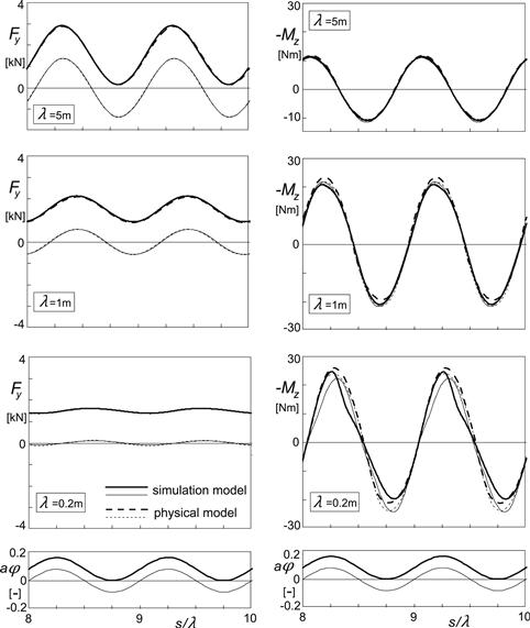
FIGURE 9.11 Side force and aligning torque responses of the nonlinear brush simulation model with flexible carcass to sinusoidal path curvature variations (turn slip at α = 0) of the wheel with an amplitude of aφ equal to 0.08 and average levels of 0 (thin curves) and 0.08 (fat curves), compared with results of the physical model (broken curves).
As a reference, the steady-state characteristics of the force and moment response to turn slip, as computed for the single row brush model with and without carcass compliance, have been shown in Figure 9.12. Up to aφ = 1/θ the aligning torque remains zero which causes the characteristics for the cases without and with flexible carcass to become identical. The remaining course of the curves for the system including carcass compliance has not been computed as that part lies outside the range of evaluation.
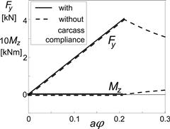
FIGURE 9.12 Steady-state turn slip force and moment characteristics of the brush model both with and without flexible carcass. The effect of tread width has not been included.
Combined Slip
To cover the case of combined slip, also including longitudinal slip, the steady-state brush model characteristics are to be adapted as formulated in Chapter 3, Section 3.2.3. In addition, the factor m that indicates the fraction of the contact length where adhesion occurs and is used to reduce the relaxation length σc is to be adapted by using the composite magnitude of slip:
![]() (9.76)
(9.76)
This expression holds because we have assumed that the brush model is isotropic. Using the magnitude of combined slip according to (9.76), the factor m can be assessed:
![]() (9.77)
(9.77)
Maurice (2000) found excellent agreement between the simulation model and the physical model for the combined slip cases: αo = 0.08 rad and ![]() = 0.08 rad and κo = 0.06 and
= 0.08 rad and κo = 0.06 and ![]() = 0.06 with a phase difference of 45° and wavelengths of 0.2, 1, and 5 m. For a more precise treatment with the interaction in the sliding range taken into account as well, we refer to the work of Berzeri et al. (1996). Adding turn slip will influence the combined slip response further. The next section approaches this matter in a pragmatic way.
= 0.06 with a phase difference of 45° and wavelengths of 0.2, 1, and 5 m. For a more precise treatment with the interaction in the sliding range taken into account as well, we refer to the work of Berzeri et al. (1996). Adding turn slip will influence the combined slip response further. The next section approaches this matter in a pragmatic way.
9.2.2 The Model Adapted to the Use of the Magic Formula
Now that we have treated all ingredients of the force and moment short wavelength responses to longitudinal, lateral, and turn slip and have developed the structure of the contact model, we may carry on and show the performance of the model adapted to the use of the Magic Formula the parameters of which may have been assessed through full scale steady-state tire measurements. The model includes the effect of tread width.
To illustrate the matter, we will here consider a simplified set of formulas for the steady-state responses, the complete version of which have been listed in Chapter 4, Sections 4.3.2 and 4.3.3. Only the case of combined side slip and turn slip will be considered. Adding braking or driving will not pose any problems.
A first problem that is encountered is the fact that in the model developed above where the contact patch is represented by the brush model, the steady-state characteristics employed belong to the brush model of the contact patch and not to the total model including the compliant carcass. In Figure 9.7 the calculated total model characteristics can be seen together with those of the contact patch alone.
An obvious solution is to model the contact patch characteristics with the Magic Formulas. These, however, will deviate from those assessed for the complete tire because the contact patch ‘sees’ a slip angle that differs (is smaller) from that of the wheel plane. A set of adapted MF parameters may be established off-line for the contact patch or an iteration loop may be included to achieve the correct steady-state behavior of the total model. A practical way has been found which employs a first-order feedback loop with a small time constant. Instead of introducing an additional first-order differential equation, the already present first-order equation for the transient side slip ![]() has been used. The diagram of Figure 9.13 illustrates the setup. A similar approach is followed in Section 9.3 to account for the camber angle of the belt being different from the camber angle of the wheel plane.
has been used. The diagram of Figure 9.13 illustrates the setup. A similar approach is followed in Section 9.3 to account for the camber angle of the belt being different from the camber angle of the wheel plane.
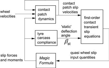
FIGURE 9.13 Diagram explaining the model structure using the Magic Formula.
The transient slip first-order differential equations listed below are identical to those derived in the previous section except for the first equation for the lateral transient slip. The factor ![]() in (9.86) accounts for the effect of tread width. Instead of using the axle velocity V, we take here the possibly more accurate velocity Vc of the contact center.
in (9.86) accounts for the effect of tread width. Instead of using the axle velocity V, we take here the possibly more accurate velocity Vc of the contact center.
![]() (9.78)
(9.78)
![]() (9.79)
(9.79)
![]() (9.80)
(9.80)
![]() (9.81)
(9.81)
![]() (9.82)
(9.82)
![]() (9.83)
(9.83)
To include camber, ![]() is to be replaced by Vcφc according to (4.76) with the subscript c (of contact patch) introduced.
is to be replaced by Vcφc according to (4.76) with the subscript c (of contact patch) introduced.
In (9.78) the calculated deflection angle has been used:
![]() (9.84)
(9.84)
![]() (9.85)
(9.85)
![]() (9.86)
(9.86)
![]() (9.87)
(9.87)
![]() (9.88)
(9.88)
![]() (9.89)
(9.89)
![]() (9.90)
(9.90)
![]() (9.91)
(9.91)
Simplified side force and aligning torque Magic Formulae (MF ed. 2):
![]() (9.92)
(9.92)
![]() (9.93)
(9.93)
![]() (9.94)
(9.94)
![]() (9.95)
(9.95)
![]() (9.96)
(9.96)
![]() (9.97)
(9.97)
![]() (9.98)
(9.98)
![]() (9.99)
(9.99)
![]() (9.100)
(9.100)
![]() (9.101)
(9.101)
![]() (9.102)
(9.102)
![]() (9.103)
(9.103)
![]() (9.104)
(9.104)
![]() (9.105)
(9.105)
![]() (9.106)
(9.106)
![]() (9.107)
(9.107)
![]() (9.108)
(9.108)
![]() (9.109)
(9.109)
Factors reduced with slip:
![]() (9.110)
(9.110)
![]() (9.111)
(9.111)
![]() (9.112)
(9.112)
![]() (9.113)
(9.113)
![]() (9.114)
(9.114)
![]() (9.115)
(9.115)
with tire composite parameter
![]() (9.116)
(9.116)
and the total magnitude of equivalent side slip
![]() (9.117)
(9.117)
where, in the present application, κ′ = 0.
Other parameter relations:
 (9.118)
 (9.119)
 (9.120)
Steady-State, Step Response, and Frequency Response Characteristics
To demonstrate the performance of the model, a number of typical characteristics will be presented. The hypothetical steady-state pure side slip and pure turn slip characteristics of the model have been given in Figure 9.14.
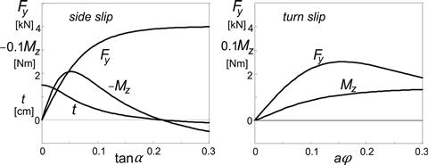
FIGURE 9.14 Steady-state side slip and turn slip force and moment characteristics of the overall tire model as defined by the Magic Formula. The effect of tread width has been included.
The step response graphs of Figure 9.15 show the proper shapes of the various curves, notably the initial horizontal tangent of the response curves of the side force to turn slip and of the moment to side slip, also shown in Figure 5.21 (no tread width). Also, the peak of the moment response curve to spin and the dip of the curve of the moment response to steer angle are exhibited, as expected.
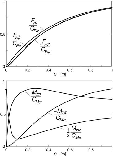
FIGURE 9.15 Step response curves of the side force and of the aligning torque to side slip α, turn slip (path curvature) φ, and steer angle ψ.
Figure 9.16 presents the frequency response functions of the linearized system at zero average side and turn slip with tread width effect included. The curves may be compared with those of the string model with tread elements, cf. Figure 5.23 (with zero tread width). In Figure 9.17 the Nyquist plots of the moment response to steer angle have been depicted. The upper diagram shows the influence of tread width by changing the parameter ![]() . If equal to zero, the thin tire is represented. The value 1 corresponds with the base line configuration. The lower graph provides insight into the influence of the parameter εφ12 that governs the magnitude of the effect of the transient yaw deflection angle αM (9.64, 9.86). The value 4 is used in the base line configuration. When compared with the plots of Figures 5.27 and 5.35, it may be concluded that the model is capable of approaching the responses of more complex infinite order (string) models and of actual tires.
. If equal to zero, the thin tire is represented. The value 1 corresponds with the base line configuration. The lower graph provides insight into the influence of the parameter εφ12 that governs the magnitude of the effect of the transient yaw deflection angle αM (9.64, 9.86). The value 4 is used in the base line configuration. When compared with the plots of Figures 5.27 and 5.35, it may be concluded that the model is capable of approaching the responses of more complex infinite order (string) models and of actual tires.
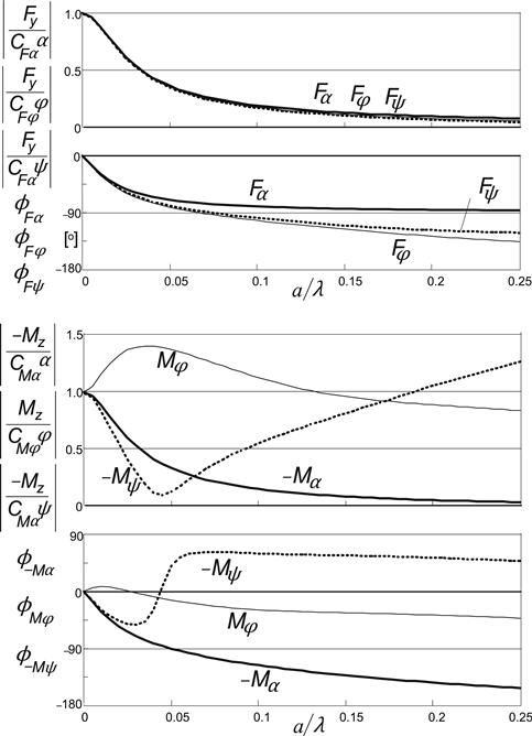
FIGURE 9.16 Frequency response function of system with tread width. Curves for the force and moment responses to side slip α, turn slip (path curvature) φ, and steer angle ψ have been indicated.
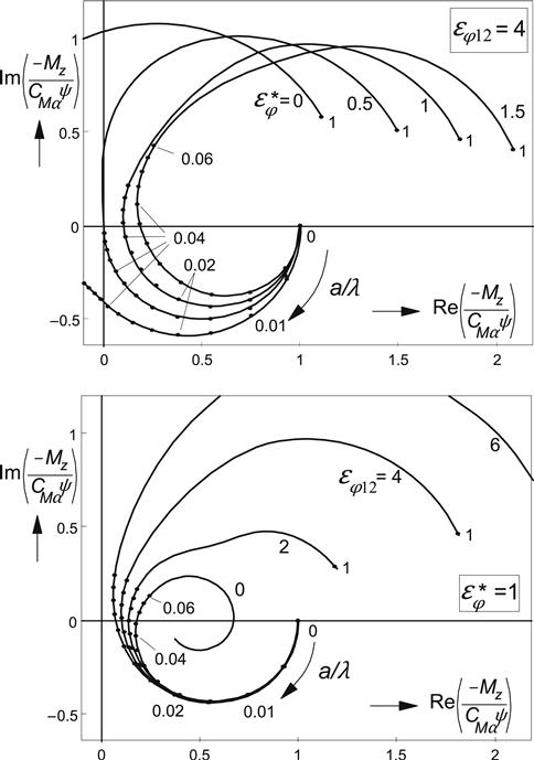
FIGURE 9.17 Nyquist frequency response plots of the aligning torque to steer angle. Upper diagram: influence of tread width (4 is base line value), lower diagram: influence of the transient yaw deflection response to turn slip (4 is base line value).
Large Slip Angle and Turn Slip Response Simulations
The same sinusoidal maneuvers have been simulated as was done before with the brush-based contact model. The complete nonlinear set of Eqns (9.78)–(9.120) has been used with parameters listed in Table 9.2.
TABLE 9.2 Parameter Values for Tire Model with Magic Formula Including Quantities Introduced Later on.
The slip angle variation is sinusoidal around average levels αo = 0 and 0.08 rad with one amplitude: ![]() = 0.08 rad at three wavelengths: λ = 0.2, 1, and 5 m. Similarly, the turn slip has two average levels: aφo = 0 and 0.08 and one amplitude:
= 0.08 rad at three wavelengths: λ = 0.2, 1, and 5 m. Similarly, the turn slip has two average levels: aφo = 0 and 0.08 and one amplitude: ![]() , also at wavelengths: λ = 0.2, 1, and 5 m.
, also at wavelengths: λ = 0.2, 1, and 5 m.
The diagrams of Figures 9.18 and 9.19 present the results. We observe that the curves are quite similar to those depicted in the Figures 9.10 and 9.11. Only, as expected, the moment response to turn slip is very much affected by the now introduced effect of the tire tread width.
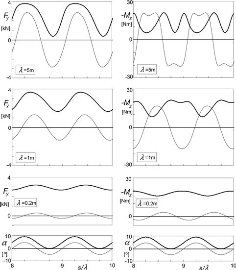
FIGURE 9.18 Side force and aligning torque responses of the Magic Formula-based simulation model with flexible carcass and finite tread width to sinusoidal slip angle variation of the wheel plane with an amplitude of 0.08 rad and average levels of 0 (thin curves) and 0.08 rad (fat curves).
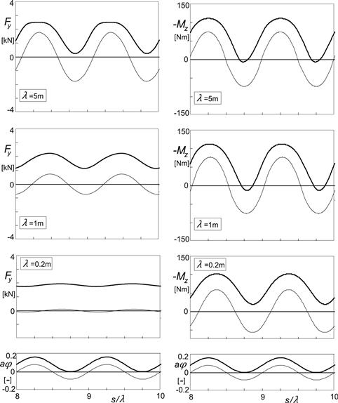
FIGURE 9.19 Side force and aligning torque responses of the Magic Formula-based simulation model with flexible carcass and finite tread width to sinusoidal path curvature variations (turn slip at α = 0) of the wheel plane with an amplitude of aφ of 0.08 and average levels of 0 (thin curves) and 0.08 (fat curves).
Maurice has conducted extensive experiments with a 205/60R15 91V tire at 2.2 bar inflation pressure on a 2.5 m drum using the pendulum test rig of Figure 9.38. The diagrams of Figure 9.20a present the computed results compared with experimental data for the case of pure side slip. The experiments have been carried out at very low speed to avoid inertia effects of the moving tire.
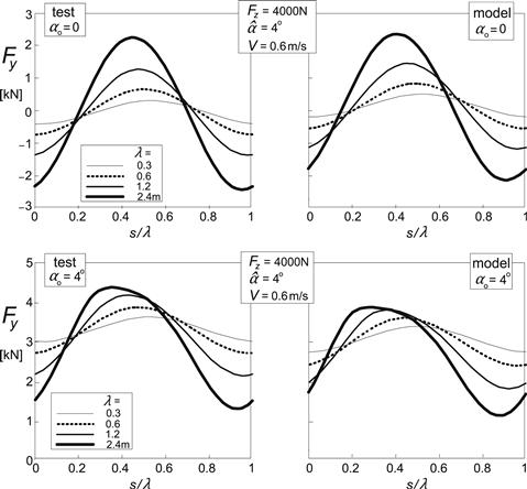
FIGURE 9.20a Comparison of theoretical model calculations and experimental results performed at 0.6 m/s on a 2.5 m drum (Maurice). The curves cover one wavelength of the periodic responses to sinusoidal slip angle variations. Force response to slip angle variations at two levels of side slip.
The wavelength ranges from 0.3 to 2.4 m. The upper diagram refers to the case of zero average slip angle and 4° amplitude. The lower diagram shows the responses around an average slip angle of 4°, which causes the curves to deviate considerably from the input sinusoidal shape.
The curves clearly show that a shorter wavelength causes the response amplitude to decrease and the phase lag to increase. It can also be observed that the responses occur more quickly at larger levels of slip, which is due to the sharp decrease of the relaxation length with increasing slip. The Magic Formula was used to model the steady-state characteristics. The parameters were obtained from separate tests performed on the drum at the much higher speed of 60 km/h. The different conditions may explain the deviation in level of the calculated responses with respect to the measured ones.
Figure 9.20b presents the comparison with the results of a second series of experiments under the same conditions. Here, the vertical load is changed sinusoidally while the slip angle is kept at a low level and at a higher level.
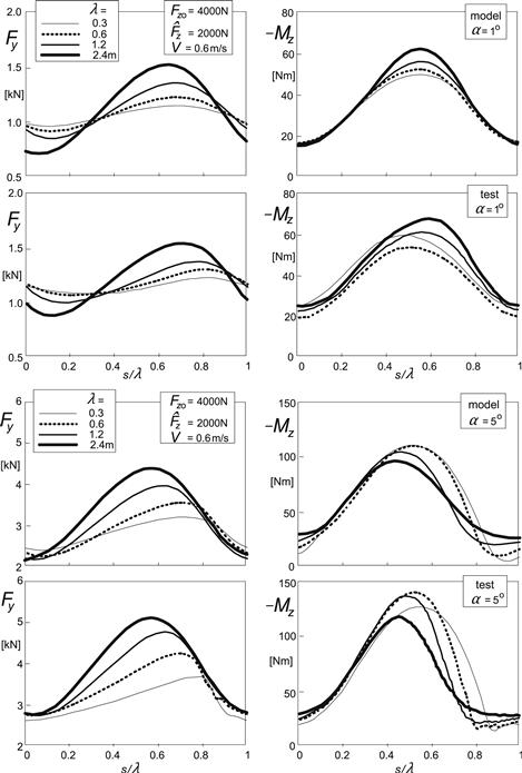
FIGURE 9.20b Comparison of theoretical model calculations and experimental results performed at 0.6 m/s on a 2.5m drum (Maurice). The curves cover one wavelength of the periodic responses to sinusoidal load variations. Force and moment response to vertical load variations at two values of slip angle.
For these experiments the measuring tower of Figure 9.37 (left) has been employed. The results are similar to those discussed in Chapter 8, Figure 8.9. The moment response seems to be improved with the more complex tire model.
The agreement of the computed results with experimental data is quite good. As has been reported by Maurice, also for the moment response a rather good agreement has been established. Since at the maximum slip angle of 8° the peak of the moment characteristic has been surpassed, the result becomes quite sensitive to small differences between actual and model steady-state characteristics of the aligning torque.
9.2.3 Parking Maneuvers
Parking maneuvers take place at very low or zero speed. The torque acting on the tire at such conditions may become very large. The influence of the finite tread width is essential as the response to spin is now predominant. We might employ the equations developed above but then we should take care of the integration of the spin velocity to properly limit the buildup of the yaw transient slip. Similar problems arose when considering the problem of braking to standstill or starting from standstill, cf. Section 8.6, Eqns (8.112, 8.113).
To achieve a much better agreement with experimental evidence, a different approach will be followed in the present application. It may be noted that an important characteristic is actually still missing. For the brush based model, Eqn (9.70) was used. The equation governs the variation of the aligning torque Mz that arises when the nonrolling tire is steered and the steer angle ψ is increased from zero to and beyond the state of full sliding. Ultimately, the torque reaches the magnitude that would also arise when the rolling tire is subjected to a constant rate of turning dψ/dt (while the slip angle remains zero) at a forward speed Vx that decreases to zero. Then, the radius of turn R reduces to zero and thus the spin approaches infinity. Figure 9.21 illustrates the situation.
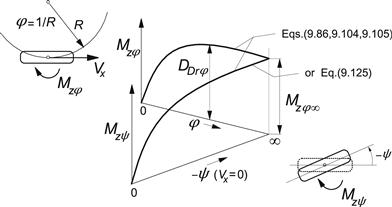
FIGURE 9.21 Approaching the maximum torque at standstill in two ways: 1. by decreasing the turn radius R to zero and 2. by increasing the steer angle −ψ while standing still.
The missing characteristic will be modeled by using a for-this-purpose adequate model that has been developed by Van der Jagt (2000). In his dissertation a model study was discussed that is especially aimed at the generation of a proper moment response to steering at very low or zero speed. First, the brush model was used to gain general insight into the phenomena that occur. Qualitatively good results have been obtained using this model, notably when a sinusoidal steer angle variation is imposed and the state of almost full sliding is attained periodically. For practical usage, a special type of model was developed of a nature completely different from the models used so far. Since this model appears to perform very well in the near zero speed range, we have tried to incorporate Van der Jagt's model in the existing model structure. For a gradual transition from the new type of model to the existing one, when the speed approaches and surpasses a low-speed threshold has been taken care of.
The principle of Van der Jagt's approach is that at a given rate of change of the steer input the growth rate of the tire angular deflection β decreases in proportion to a function of the remaining difference between the maximum achievable deflection and the current deflection. The torsional stiffness is assumed to be a constant and the resulting characteristic of the torque becomes similar to a first-order response function. The calculated moment gradually approaches its maximum value. When the direction of rotation of the wheel about the vertical axis is changed, the distance to the new, opposite, peak torque is large and, accordingly, the rate of reduction of the moment is large as well. It is this feature of the model that is attractive since a similar behavior has been found to occur with the actual tire subjected to an alternating left and right sequence of turning. The equations that govern the moment generation at standstill are as follows:
![]() (9.121a)
(9.121a)
![]() (9.121b)
(9.121b)
![]() (9.121c)
(9.121c)
For the parameter value co = 2, Figure 9.22 presents the calculated variation of the torque vs the steer angle compared with experimentally obtained results as reported by Van der Jagt. The nonrolling tire (size P205/65R15) is loaded to 4800 N on a flat plate and subsequently steered at a rate of + and −1 deg./s. The correspondence is quite good except perhaps for the initial phase where the wheel starts to be steered from the condition where Mz = 0. To improve the model performance Van der Jagt suggests using an exponent co, the value of which depends on the last extreme of the deflection angle β. For possible further refinements of the model, we refer to the original work.
When, instead of the new approach, the Magic Formula would be used with the integration limitation as suggested according to Eqns (8.112, 8.113), a sharp peak would arise in the curve where the direction of turning is changed. As a result, the moment decreases at a much slower rate than shown by the test result.
The problem is now how to integrate the new model feature in the original model structure. The transient slip quantity ![]() , Eqn (9.86), may be recognized to be proportional to the deflection angle. As can be seen from Eqns (9.80, 9.82, 9.83, and 9.86) this quantity is obtained through integration of
, Eqn (9.86), may be recognized to be proportional to the deflection angle. As can be seen from Eqns (9.80, 9.82, 9.83, and 9.86) this quantity is obtained through integration of
![]() (9.122)
(9.122)
In the new configuration, the integration is conducted at a gradually decreasing rate while approaching the maximum torque value. We have
![]() (9.123)
(9.123)
![]() (9.124)
(9.124)
At zero speed wVlow = 1. The moment is found with the linear function, cf. (9.104):
![]() (9.125)
(9.125)
For the standing tire with speed Vx equal to zero, the response to alternating steer angle variations will follow a course similar to that of Figure 9.22.
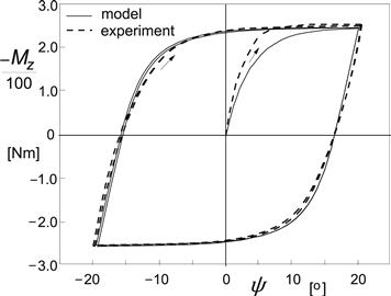
FIGURE 9.22 Calculated and experimentally assessed variation of the moment vs steer angle for a nonrolling tire pressed against a flat plate at a load Fz = 4800 N.
It is now desired to change gradually to the original equations when the tire starts rolling. The transition is accomplished by adding up the following two components. The first one decreases in magnitude with increasing speed until it vanishes at Vx = Vlow while the second part increases from zero to its full value also at Vx = Vlow. For the gradual change, the following speed window is used:
![]() (9.126)
(9.126)
With this quantity (already used in (9.123)), the first part that prevails at low speed becomes
![]() (9.127a)
(9.127a)
and the fraction obtained from the original (here simplified) Eqns (9.105 and 9.104)
![]() (9.127b)
(9.127b)
The resulting expression for the spin moment now reads
![]() (9.128)
(9.128)
A similar method may be employed to improve the low-speed model for the side force responding to lateral motions of the contact patch (cf. Figure 9.29, point S) and for the fore- and-aft force to longitudinal motions of the same point S.
The adapted model will now be applied to the simulation of the motion of a rigid quarter car model with mass mqc that, while a sinusoidal steering input is applied, starts moving after 1.6 s with a linearly increasing speed. The lateral acceleration of the quarter car axle results from the action of the side force that begins to develop after the wheel has started to roll:
![]() (9.129)
(9.129)
The lateral wheel slip velocity is now not only a result of the yaw angle at a forward speed of the vehicle ![]() but also due to the lateral velocity of the wheel axle
but also due to the lateral velocity of the wheel axle ![]() . We have
. We have
![]() (9.130)
(9.130)
which serves as an input into the Eqns (9.88 and 9.91). The additional parameter values have been appended in Table 9.2.
Figure 9.23 shows the courses of variation of various quantities vs time. Simultaneously, in Figure 9.24, the moment is plotted vs steer angle. Several phenomena occur that deserve to be noted. The steer angle has an amplitude that is large enough to attain a level of the moment close to its maximum. The moment starts to decrease in magnitude as soon as the steer angle passes its peak value. The moment changes sign before the steer angle does the same. After 1.6 s, the forward speed increases linearly with time and the side force starts to build up as a result of the slip angle that begins to develop. The car shows a lateral vibration in the low speed range as indicated by the fluctuations of the side force. Evidently, the quarter car vibrates against the lateral tire stiffness. The moment amplitude decreases as the spin diminishes in amplitude due to the increasing speed. The side force amplitude increases because of the larger lateral oscillations of the quarter car mass induced by the increasing speed of travel at the constant steer input pattern with time. The loops shown in Figure 9.24 give a nice impression of the transition from the situation at standstill to the condition at higher speeds. At standstill the moment varies in accordance with the diagram of Figure 9.22.
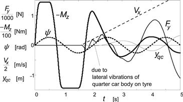
FIGURE 9.23 Simulation results of a parking maneuver (car leaving the parking lot while steering sinusoidally).
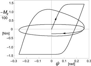
FIGURE 9.24 The steer torque plotted vs steer angle during the maneuver of Figure 9.23.
As mentioned before, to get a more accurate calculation of responses to lateral and circumferential wheel displacements at or near forward speed equal to zero, one might apply, instead of the abrupt integration limitation suggested earlier, Eqns (8.112) and (8.113), the same structure of additional Eqns (9.123) and (9.124), and an adaptation such as achieved in Eqn (9.128).
9.3 Tire Dynamics
The contact patch model has been used above in connection with a flexible carcass. In the present section the inertia of the belt will be introduced. Since we restrict the application of the model to frequencies lower than ca. 60 Hz the belt may be approximated as a rigid ring that is attached to the wheel rim through flexible sidewalls. To ensure that the total static tire stiffness remains unchanged, residual springs have been introduced between the contact patch and the belt. In certain cases, a bypass spring directly connecting the rim and the contact patch may be needed to improve model accuracy.
9.3.1 Dynamic Equations
As depicted in Figure 9.25, the wheel axle position is defined by the location of the wheel center (X,Y,Z) and orientation (γ,θ,ψ). The wheel speed of revolution is denoted by Ω. A moving axes system (C,x,y,z) has been defined of which the x axis points forwards and runs along the line of intersection of the wheel plane and the road plane. The y axis lies in the plane normal to the road plane and passing through the wheel spin axis. The z axis forms the normal to the road surface. The origin of the moving triad is the contact center C. Another moving system of axes (A,ξ;,η,ζ) is introduced of which the origin A is located in the wheel center, the ξ; axis is horizontal, and the η axis runs along the wheel spindle axis. With respect to the wheel rim the belt shows relative displacements: ![]() and
and ![]() . The contact patch is displaced horizontally with respect to the belt corresponding to the deflections of the residual springs:
. The contact patch is displaced horizontally with respect to the belt corresponding to the deflections of the residual springs: ![]() and
and ![]() . The superscript r designates a relative displacement; without the superscript we have the displacement with respect to the inertial system (X,Y, Z). All relative displacements are considered small and the dynamic equations may be linearized.
. The superscript r designates a relative displacement; without the superscript we have the displacement with respect to the inertial system (X,Y, Z). All relative displacements are considered small and the dynamic equations may be linearized.
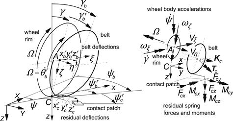
FIGURE 9.25 Model structure featuring contact patch, residual compliance, rigid belt, carcass compliance, and wheel rim.
The wheel motion forms the input to the tire system (possibly together with the road profile). From these, the wheel velocities Vξ;, Vη, and Vζ and ωξ;, ωη, and ωζ (defined with respect to the axle triad (A,ξ;,η,ζ)) or alternatively ![]() (defined with respect to the moving contact triad (C,x,y,z)) and the camber angle γ and the radial tire deflection ρz are available. The camber angle γ will be treated here as a small quantity.
(defined with respect to the moving contact triad (C,x,y,z)) and the camber angle γ and the radial tire deflection ρz are available. The camber angle γ will be treated here as a small quantity.
The belt considered as a rigid circular body has a mass mb and moments of inertia Ibx,y,z. The carcass (sidewalls) possesses stiffnesses cbx,y,z and damping coefficients kbx,y,z. In the figure the force and moment vectors Kc and Tc defined to act from contact patch to and about the center of the belt have been indicated. Their components are defined with respect to the (A,ξ;,η,ζ) triad. The first of the two sets of first-order differential equations for the six degrees of freedom reads:
![]() (9.131)
(9.131)
![]() (9.132)
(9.132)
![]() (9.133)
(9.133)
![]() (9.134)
(9.134)
![]() (9.135)
(9.135)
![]() (9.136)
(9.136)
Several coupling terms show up. These are due to the gyroscopic effect and due to the action of the rotating radial dampers with resulting coefficient kbx = kbz and the lateral dampers with resulting angular damping coefficients kbψ = kbγ. Figure 9.26 illustrates the mechanism that gives rise to the interaction terms. The example concerns the term ![]() in (9.131). The following relations between the two sets of wheel and axle angular velocities hold:
in (9.131). The following relations between the two sets of wheel and axle angular velocities hold:
![]() (9.137)
(9.137)
![]() (9.138)
(9.138)
![]() (9.139)
(9.139)
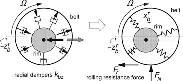
FIGURE 9.26 The rotating radial dampers of the vertically deflected tire gives rise to a resulting fore-and-aft force acting between the belt and the rim. The resulting longitudinal deflection produces a rolling resistance force Fr through the action of the normal load FN.
For the relative displacements between belt and wheel rim we have the second set of six first-order differential equations:
![]() (9.140)
(9.140)
![]() (9.141)
(9.141)
![]() (9.142)
(9.142)
and
![]() (9.143)
(9.143)
![]() (9.144)
(9.144)
![]() (9.145)
(9.145)
The forces and moments appearing in the right-hand members of Eqns (9.131–136) can be expressed in terms of the forces acting in the residual springs that connect the contact patch with the belt.
The residual spring concept as defined in the model has been addressed in greater detail in Figure 9.27. The left-hand top diagram presents an analogous dynamic system exhibiting n vibrational modes, each belonging to one of the n modal components. The system is formed by a chain of n single mass–spring systems, which are connected by common force joints (realized by rope and pulleys). For a tire, the first mass represents the rigid belt. The remaining modal components with higher natural frequencies show vibrational modes with the belt exhibiting deflections distributed along its circumference. When neglecting the inertias of these higher order modal components (top right diagram), the residual spring remains with compliance equal to the sum of the series of the n−1 individual compliances. The middle right diagram shows that attaching the residual spring to the rigid belt results in the correct vertical stiffness and natural frequency of the loaded and the free tire/wheel (cf. Figure 9.40). The lower diagrams of Figure 9.27 indicate the introduced residual springs that connect the belt with the contact patch body in circumferential, vertical, lateral, and yaw directions.
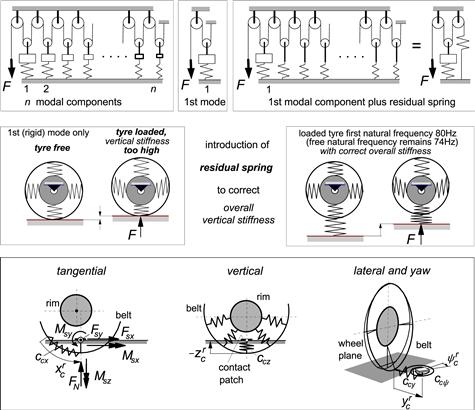
FIGURE 9.27 Top: Analogous system with n modes of vibration; reduction to system with one natural mode plus residual stiffness. Middle: Illustration of reduced system without and with residual vertical spring. Bottom: Four residual springs introduced in the tire model; deflections of the residual springs attaching the contact patch to the belt.
The directions of the residual spring forces and moments are defined to act in parallel to the moving axes system (C,x,y,z) with the z axis normal to the road plane. Also, the vertical forces Fz are defined here, in contrast to the definition adopted in the remainder of this chapter and in Chapter 10, according to the consistent SAE convention. For the normal wheel load acting from road to tire we introduce the positive quantity FN. We have in case of a horizontal road plane with products of angles neglected and rl denoting the loaded radius:
![]() (9.146)
(9.146)
![]() (9.147)
(9.147)
![]() (9.148)
(9.148)
![]() (9.149)
(9.149)
![]() (9.150)
(9.150)
![]() (9.151)
(9.151)
Obviously, a proper axes transformation is to be performed if the road plane is not horizontal. As a result, transverse and forward slopes will affect the terms appearing in the right-hand members of Eqns (9.146–9.151). It is left to the user to introduce these transformations.
The contact patch body is subjected to forces acting in the residual springs (subscript c) and external forces acting from road surface to contact patch (subscript s). Figure 9.28 illustrates the situation. The contact inertia increases the total order of the system. The introduction of the inertia may be avoided, while maintaining integrational causality, by considering the ‘residual’ damper not as a resistor but as a conductor. The differential equations that govern the horizontal dynamics of the contact patch body read:
![]() (9.152)
(9.152)
![]() (9.153)
(9.153)
![]() (9.154)
(9.154)
and in addition, equations for the residual deflections
![]() (9.155)
(9.155)
![]() (9.156)
(9.156)
![]() (9.157)
(9.157)
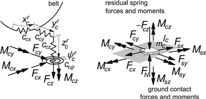
FIGURE 9.28 Internal and external forces and moments acting on the contact patch body.
Also here, in the right-hand members, a road slope will have an effect. An axes transformation is needed to introduce properly the belt velocities with respect to the location of the contact patch. From the deflections and deflection rates the residual spring and damper forces appearing in Eqns (9.146–9.151) can be determined. We have
![]() (9.158)
(9.158)
![]() (9.159)
(9.159)
![]() (9.160)
(9.160)
while
![]() (9.161)
(9.161)
![]() (9.162)
(9.162)
![]() (9.163)
(9.163)
The contact forces and moments result from the contact slip model equations developed in the preceding section. The computed forces and moments have been defined according to the Magic Formula model, which at steady state, act with respect to the moving axes system (C,x,y,z). These forces and moments, here provided with subscript C, are to be transformed to arrive at the set of forces and moments defined according to the system with lines of action shifted sideways over the calculated ‘static’ lateral displacement ![]() of the contact patch with respect to the wheel plane. These corrected quantities correspond to the forces and moments provided with subscript S occurring in the Eqns (9.152–9.154) and (9.161–9.163):
of the contact patch with respect to the wheel plane. These corrected quantities correspond to the forces and moments provided with subscript S occurring in the Eqns (9.152–9.154) and (9.161–9.163):
![]() (9.164)
(9.164)
![]() (9.165)
(9.165)
![]() (9.166)
(9.166)
![]() (9.167)
(9.167)
![]() (9.168)
(9.168)
![]() (9.169)
(9.169)
where the static lateral deflection is computed from the side force and the overall lateral compliance of the standing tire at ground level:
![]() (9.170)
(9.170)
With the transient response variables computed with the aid of Eqns (9.78–9.86) plus Eqn (9.20) the contact forces and moments may be found by using these variables as argument in the steady-state equations presented in Sections 4.3.2 and 4.3.3. However, we should properly account for the response to a varying camber angle of the belt plane.
For this purpose, we introduce the tire total spin velocity ![]() , cf. Eqn (4.76), which has been corrected for the static belt camber deflection to enable the direct use of the relevant magic formulas (analogous to the use of βst in Eqn (9.78)):
, cf. Eqn (4.76), which has been corrected for the static belt camber deflection to enable the direct use of the relevant magic formulas (analogous to the use of βst in Eqn (9.78)):
![]() (9.171)
(9.171)
with the ‘static’ belt deflection angle (neglecting the action of Mx)
![]() (9.172)
(9.172)
Further, we write instead of βst:
![]() (9.173)
(9.173)
The transient slip first-order differential equations are repeated below. They are identical to Eqns (9.78–86) plus Eqn (9.20) except for the now-added effect of the camber angle in the right-hand members. In (9.20)![]() may be replaced by
may be replaced by ![]() as at steady state, these are equal for the contact patch and overall tire model. The same holds for the spin variables
as at steady state, these are equal for the contact patch and overall tire model. The same holds for the spin variables ![]() and
and ![]() . The input slip velocities have been indicated in Figure 9.29.
. The input slip velocities have been indicated in Figure 9.29.
![]() (9.174)
(9.174)
![]() (9.175)
(9.175)
![]() (9.176)
(9.176)
![]() (9.177)
(9.177)
![]() (9.178)
(9.178)
![]() (9.179)
(9.179)
![]() (9.180)
(9.180)
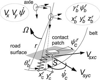
FIGURE 9.29 Slip velocities of contact patch forming input to transient slip equations.
In addition, we need the composite transient slip quantities:
![]() (9.181)
(9.181)
![]() (9.182)
(9.182)
The slip variables employed in the Magic Formulas (MF) are replaced by the transient slip variables as indicated in the arguments of the following expressions:
![]() (9.183)
(9.183)
![]() (9.184)
(9.184)
![]() (9.185)
(9.185)
![]() (9.185a)
(9.185a)
![]() (9.186)
(9.186)
![]() (9.187)
(9.187)
![]() (9.188)
(9.188)
![]() (9.189)
(9.189)
![]() (9.190)
(9.190)
![]() (9.191)
(9.191)
Eqn (9.188) has been added, which is in agreement with the short wavelength transient slip theory, cf. Eqns (9.106 and 9.110). The input to the transient slip Eqns (9.171, 9.174–9.180) is constituted by the velocities of the contact patch, cf. Eqns (9.152–9.154), Figure 9.29:
![]() (9.192)
(9.192)
![]() (9.193)
(9.193)
![]() (9.194)
(9.194)
The overturning couple Mx can be modeled with the function (4.E69) where the Fy part may be replaced by the expression (4.122–4.124) with transient slip angle as argument, if the actual momentary loaded radius rl (distance between points A and C) has been properly accounted for in the (steady-state) measurements and further processing. The wheel load FN (=|Fz|) and the rolling resistance moment My depend on the radial deflection and on a number of other variables. The subsequent section provides information on the experimentally assessed functional relationships.
Finally we need to establish the output forces and moments that act from the tire upon and about the wheel center. These quantities are denoted with the symbols K and T and are provided with the subscript a. The components are defined to act along and about the axes of the axle triad (A, ξ;,η,ζ). We find
![]() (9.195)
(9.195)
![]() (9.196)
(9.196)
![]() (9.197)
(9.197)
![]() (9.198)
(9.198)
![]() (9.199)
(9.199)
![]() (9.200)
(9.200)
where the forces and moments acting from belt center to rim are retrieved from Eqns (9.131–9.136):
![]() (9.201)
(9.201)
![]() (9.202)
(9.202)
![]() (9.203)
(9.203)
![]() (9.204)
(9.204)
![]() (9.205)
(9.205)
![]() (9.206)
(9.206)
Values of inertia parameters normalized with tire mass mo and reference moment of inertia ![]() , with ro the unloaded tire radius, have been listed in Appendix 3.
, with ro the unloaded tire radius, have been listed in Appendix 3.
9.3.2 Constitutive Relations
In the study of Zegelaar (1998) important observations have been made regarding contact area dimensions, static and dynamic vertical stiffness, and characteristics at different speeds of rolling, static longitudinal stiffness of the standing tire, tire radius growth with speed, rolling resistance, effective rolling radius, and rolling resistance couple. Much of the results will be repeated below.
Dimensions of the Contact Area
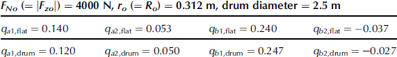
Prints of the contact patch may be obtained by using ink or carbon paper. The shape appears to change from an oval shape at very low normal loads to a more rectangular shape at higher values of the load. An effective rectangular contact area may be defined with an area equal to that of the envelope of the actual print. The ratio of the width and length of the rectangle is taken equal to that of the actual contact area. The effective half length and half width are denoted as a and b. The dimensions depend on the normal load FN (=|Fz|) and the following formulas have been found to give a good approximation:
![]() (9.207)
(9.207)
and
![]() (9.208)
(9.208)
with ro denoting the free tire radius. Figure 9.30 presents the curves compared with the measured effective quantities for the tire pressed on a flat surface and on a curved drum surface with 2.5 m diameter. Obviously, the results are satisfactory. The dimensions of the tire were again: 205/60R15 91V at 2.2 bar inflation pressure. The nondimensional parameter values can be found in Table 9.3. In App. 3(3) an alternative expression for a is presented based on the radial deflection ρz instead of on the normal load FN. The resulting value is much less dependent on the possibly changed inflation pressure.
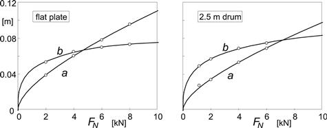
FIGURE 9.30 Measured and calculated half length a and half width b of the contact patch vs wheel load, for the cases: loading on a flat plate and on a drum surface.
TABLE 9.3 Parameter Values for Contact Patch Dimensions (205/60R15 91V at 2.2 bar)
The Sidewall Stiffnesses and Damping
The rigid ring model of the tire freely rolling and loaded on the road shows three in-plane modes of vibration: the vertical mode and two angular modes. One of these rotational modes vibrates in phase with rim angular vibration while the other moves in anti-phase. The natural frequencies have been estimated with the aid of experiments conducted on the drum test stand where the wheel, at fixed axle position, rolls over a short cleat or is excited by brake torque fluctuations, cf. Section 9.4.2.
The experiments indicate that the natural frequencies lying in the range of 0–100 Hz decrease with velocity. Other researchers found the same tendency, notably Bruni, Cheli and Resta (1996). Since the sidewall stiffnesses are much larger than the residual stiffnesses it is decided to make the in-plane sidewall stiffnesses dependent on the speed of rolling. As to the out-of-plane vibrations, Maurice did not ascertain the necessity to make the lateral, yaw, and camber stiffnesses speed dependent.
Zegelaar introduces a variable quantity QV that is a measure of the time rate of change of the loaded tire deformation due to rolling. We have the nondimensional quantity (Vo representing the reference velocity, cf. Section 4.3.2):
![]() (9.209)
(9.209)
The following expressions for the sidewall stiffnesses have been found to be appropriate:
![]() (9.210)
(9.210)
![]() (9.211)
(9.211)
![]() (9.212)
(9.212)
The additional subscript 0 designates the situation of the loaded nonrotating tire. The vertical and longitudinal stiffnesses have been assumed equal to each other. The parameters qbVx,z,θ govern the speed dependency of the stiffnesses.
The sidewall damping coefficients kbi = kbx,y,z,γ,θ,ψ are considered to be constant quantities. The interaction terms appearing in Eqns (9.131–9.136) containing the coefficients kbiΩ are omitted since these terms affect the rolling resistance and the aligning torque (also in steady state) and would make these speed dependent. The introduction of material damping being inversely proportional with frequency would be closer to reality. Further on, the rolling resistance will be introduced in an alternative, better controlled way.
For the constant stiffnesses, nondimensional parameters may be introduced. We define with FNo, ro (=Ro) and mo (the reference load, free tire radius, and tire mass) the nondimensional parameters q:
![]() (9.213)
(9.213)
![]() (9.214)
(9.214)
![]() (9.215)
(9.215)
![]() (9.216)
(9.216)
To provide more damping when the wheel speed gets close to zero, we may follow the theory of Chapter 7 and introduce kV,low as demonstrated in Chapter 8, Eqns (8.127, 8.128), where the slip speed Vsx may be replaced by Vsxc. In a similar way the residual stiffness and damping parameters cc and kc have been normalized.
The Normal Force
The spring with residual stiffness ccz indicated in Figure 9.27 hides a structure that is a lot more complex than a spring with constant stiffness. Experiments reveal that the force deflection characteristics are nonlinear: the force develops after contact has been made and increases slightly more than proportionally with the overall normal deflection ρz. Also, the tire grows with speed due to centrifugal action. Figure 9.31 illustrates both phenomena. Furthermore, it has been found useful to introduce Fx and Fy interaction terms in the vertical stiffness, cf. Reimpell et al. (1986). The following formula is proposed for the normal force including interaction and overall stiffness and growth functions (also see Eqn (4.E68) for the influence of inflation pressure):
![]() (9.217)
(9.217)
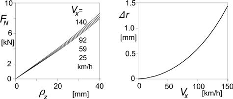
FIGURE 9.31 Vertical load vs normal deflection characteristics at various forward velocities and tire radius growth with speed.
With radius rc of assumed circular cross-sectional contour, the deflection becomes at wheel camber angle γ (relative to normal to road plane), also cf. Eqn (7.46):
![]() (9.218)
(9.218)
The tire radial growth changes quadratically with rotational velocity:
![]() (9.219)
(9.219)
Here, ro denotes the radius of the free nonrotating tire, rl the loaded radius (distance between wheel center and contact center), and Δr the increase in free tire radius due to wheel rotation velocity. The nondimensional parameter qV1 governs the influence of tire growth, qV2 the stiffness variation with speed, qFcx,y1 the interaction with horizontal forces, and qFz1,2,3 the stiffness and nonlinearity of the force deflection characteristic at zero speed and zero horizontal forces. Appendix 3 presents the parameter values fitted to experimental data. To radically simplify (9.218), we may for small γ, replace rc by ro−rl + Δr which is the calculated tire radial deflection.
From the overall characteristics the properties of the residual spring are to be derived. An exact functional relationship may be established but it can be found that the residual normal spring characteristic can be approximated by the third degree polynomial function:
![]() (9.220)
(9.220)
with the FN-related normal residual spring deflection (taking into account geometrical interaction terms with horizontal deflections)
![]() (9.221)
(9.221)
Here, ![]() is the radial displacement of the center of the belt ring with respect to the wheel center and ρx,y represent the longitudinal and lateral tire contact deflections. The actual loaded radius rl results from the calculated deflections (cf. Figure 4.30 for measured evidence) with camber influence included:
is the radial displacement of the center of the belt ring with respect to the wheel center and ρx,y represent the longitudinal and lateral tire contact deflections. The actual loaded radius rl results from the calculated deflections (cf. Figure 4.30 for measured evidence) with camber influence included:
![]() (9.222)
(9.222)
The coefficients appearing in (9.220) can be expressed in terms of sidewall stiffness cbz and wheel speed of revolution Ω:
![]() (9.223)
(9.223)
![]() (9.224)
(9.224)
![]() (9.225)
(9.225)
where, with Reimpell's terms in (9.217) omitted, we obtain
![]() (9.226)
(9.226)
![]() (9.227)
(9.227)
where the nondimensional parameters qV2 and qFz1,2,3 of Eqn (9.217) appear. The horizontal tire deflections at road surface level with respect to the wheel rim are (at small camber):
![]() (9.228)
(9.228)
![]() (9.229)
(9.229)
Appendix 3 provides the relevant parameter values for the passenger car tire that has been tested.
Free Rolling Resistance
Experiments show that the rolling resistance force Fr (pointing backward) is proportional to the tire normal load FN. A history on this subject can be found in the publication of Clark (1982). We have
![]() (9.230)
(9.230)
The rolling resistance coefficient fr depends on the forward speed and may be expressed in terms of powers of the speed, cf. Mitschke (1982):
![]() (9.231)
(9.231)
Parameter qsy1 governs the initial level of the rolling resistance force and typically lies in between 1 and 2%. Parameter qsy3 controls the slight slope of the resistance with speed. The last parameter qsy4 represents the sharp rise of the resistance that occurs after a relatively high critical speed is surpassed. Then, the so-called standing waves show up as a result of instability, cf. Pacejka (1981), or according to an alternative theory due to resonance, cf. Brockman and Braisted (1994). The formation of standing waves gives rise to large deflection variations and considerable energy loss. The phenomenon may result in failure of the tire and poses an upper limit to the safe range of operation of the tire.
Below, we will see that the rolling resistance will be introduced in the tire model through the rolling resistance moment that is imposed on the tire belt ring as an external torque about the y axis, cf. Eqn (9.236).
Effective Rolling Radius, Brake Lever Arm, Rolling Resistance Moment
In Chapter 8 the notion of the effective rolling radius has been introduced. Figure 8.12 shows the results of experiments of tires running over a drum surface. In Subsection 8.3.1 the theory is restricted to a linearized representation of the variation of the effective rolling radius with radial defection. The complete nonlinear variation versus normal load FN may be described by the expression:
![]() (9.232)
(9.232)
with
![]() (9.232a)
(9.232a)
and the vertical stiffness of the standing tire at nominal load FNo, as derived from Eqn (9.217):
![]() (9.232b)
(9.232b)
In App. 3, Eq. (A3.4), an alternative expression has been given. The longitudinal slip velocity is defined with re introduced as the slip radius, cf. e.g. Eqn (8.32).
In the present model with the belt ring and contact patch modeled as separate bodies, the longitudinal slip velocity Vsxc of the contact patch is used as input in the transient slip differential Eqn (9.174). In Eqn (9.192) with (9.155), the effective rolling radius re accomplishes the transmission of the rotational speed of the belt to the residual deflection rate of change. At steady-state condition, the deflection rates vanish and we have the following relation for the longitudinal slip speed:
![]() (9.233)
(9.233)
We may consider the power balance of a wheel subjected to a propulsion torque MD and a drag force FD acting backward on the wheel in its center. Figure 9.32 depicts the situation. The connected power flow diagram is presented in Figure 9.33. The S represents a power source (the engine) and the Rs are resistors where energy is dissipated. The balance of power requires that the equation holds:
![]() (9.234)
(9.234)
or with (9.233) and Fx = FD
![]() (9.235)
(9.235)
where ![]() represents the energy dissipating moment due to rolling. This equation suggests, at least for the model employed, that the moment arm equals the effective rolling radius (defined at zero driving or braking torque: free rolling). Consequently, the block named ‘tire' in the diagram of Figure 9.33 represents, when unfolding the bond graph, a junction structure containing a transformer with modulus re that transforms the angular speed into (a part of) the slip speed and, in the opposite direction, the slip force into the drive torque.
represents the energy dissipating moment due to rolling. This equation suggests, at least for the model employed, that the moment arm equals the effective rolling radius (defined at zero driving or braking torque: free rolling). Consequently, the block named ‘tire' in the diagram of Figure 9.33 represents, when unfolding the bond graph, a junction structure containing a transformer with modulus re that transforms the angular speed into (a part of) the slip speed and, in the opposite direction, the slip force into the drive torque.
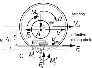
FIGURE 9.32 The driven tire–wheel combination with deflected belt and residual spring.
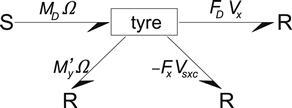
FIGURE 9.33 Power flow diagram (bond graph) of driven tire–wheel combination in steady state.
Experiments have been carried out by Zegelaar on both the flat plank machine and the drum test stand to establish the effective rolling radius and the moment arm. In these tests, a (brake) torque was applied to the wheel. The moment arm may be termed as the brake lever arm. The diagrams of Figure 9.34 have been obtained from tests performed at zero speed (for assessing the brake lever arm) and at very low speed of travel (for finding the effective rolling radius). Especially in case of the flat surface, an excellent agreement has been found to occur. It is assumed that the growth of the effective rolling radius with speed is equal to that of the free tire radius, cf. Eqn (9.219).
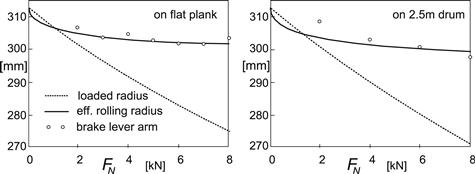
FIGURE 9.34 Tire radii as function of the normal load measured at zero or very low speed.
The diagrams of Figure 9.35 present the influence of speed on the two radii. The loaded radius has been kept fixed so that the vertical load rises when the speed is increased. Three different axle heights have been selected corresponding to the indicated initial vertical loads at zero speed FNo. The left-hand diagram shows the degree of fit for the effective rolling radius. The right-hand diagram shows the correspondence with the brake lever arm. The tests from which the brake lever arm can be assessed have been conducted at low levels of the average and the standard deviation of the brake torque random input (120 and 22 Nm, respectively). The brake lever arm results from the longitudinal force response to the imposed brake torque variation at zero frequency. The influence of the average brake torque on the ratio of the torque amplitude and the force amplitude at zero frequency, –dMB/dFx, is given in Figure 9.36. This ratio does not appear to be a constant. Especially at low loads and relatively large braking forces, large deviations arise from the value of the effective rolling radius. Note that, due to its definition, the effective radius is not affected by the magnitude of the brake force.
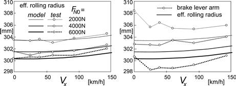
FIGURE 9.35 Tire radii measured on 2.5 m drum as a function of the forward speed at three axle heights corresponding to the indicated initial loads. Average level and amplitude of brake torque are small.
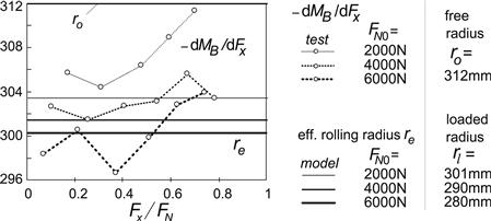
FIGURE 9.36 Ratio of brake torque increment to brake force increment as a function of level of brake force at a velocity of 25 km/h and three different axle heights (loaded radii).
With the effective radius adopted as the brake or driving torque moment arm, we find from Eqn (9.235) that if MD = 0 the moment ![]() .
.
For the (forward) rolling tire, this moment is assumed to be independent of Fx and MD. Furthermore, we obtain, at Ω = 0 where the moment due to rolling ![]() , that MD = Fxre. Obviously re is the brake lever arm corresponding with the experimental result.
, that MD = Fxre. Obviously re is the brake lever arm corresponding with the experimental result.
By considering the equilibrium about the wheel axis A, the rolling resistance moment My (acting about the C-y axis) becomes
![]() (9.236)
(9.236)
with Fr given by Eqn (9.230). Apparently, at free rolling (MD = 0) where Fx = −Fr, we correctly have: My = Frrl.
It is clear that theoretical modeling of the mechanism behind the generation of the rolling resistance moment deserves more study. In Chapter 4 the empirical formula Eqn (4.E70) has been presented for My that is based on tire test data.
9.4 Dynamic Tire Model Performance
A number of experiments have been conducted at the Delft University of Technology to assess the parameters of the dynamic model and to judge its performance. The steady-state side slip, longitudinal slip, camber force, and moment characteristics have been typically assessed from over–the-road experiments with the Delft TireTest Trailer. For the model performance evaluation, steady-state characteristics have been used, obtained from tests carried out on the drum with the strain gauge-equipped measuring hub mounted in the measuring tower, cf. Figure 9.37.
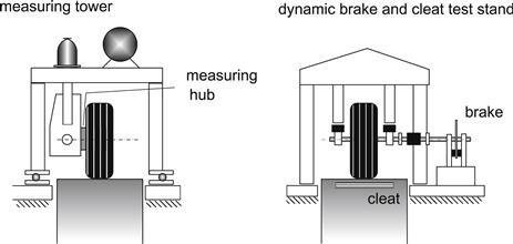
FIGURE 9.37 Principal setup of the measuring tower and of the dynamic brake and cleat test stand.
In Section 9.4.1 the dedicated dynamic test facilities have been discussed, followed by Section 9.4.2 with the presentation of the model dynamic behavior in comparison with experimental data. In Chapter 10 the model will be extended to include the description of running over road obstacles (cleats). This model extension is followed by the presentation of experimental results compared with model behavior.
The reader is referred to Chapter 12 for a more extensive description of steady-state- and higher frequency test facilities including the dedicated rigs mentioned in the section below. For some practical details regarding parameter assessment for advanced dynamic tire models, Section 10.2 may be of interest. In this context, it is important to note that cleat tests are most useful to determine both the in-plane and the out-of-plane natural frequencies of the model. Also modal testing of the unloaded tire with a fixed wheel axle may provide useful, possibly additional, information.
9.4.1 Dedicated Dynamic Test Facilities
Dynamic Brake and Cleat Test Rig
Experiments have been conducted on the 2.5 m steel drum test stand provided with a specially designed rig equipped with a disc brake installation, cf. Figure 9.37 (right-hand diagram), and for more details: Chapter 12, Figure 12.7. Brake torque fluctuation tests (Section 9.4.2) and dynamic cleat tests (Section 10.2) have been carried out. The test facilities with numerous experimental and simulation results have been described in detail by Zegelaar (1998).
The wheel axle height can be adjusted to select the tire initial load. During the tests, the axle position is held fixed causing the wheel load to rise with increasing speed. The wheel axle bearing supports are equipped with piezoelectric load cells. Steady-state- or average force levels cannot be measured very well with these force transducers. To provide an indication of the actual load increase with speed as measured in the measurement tower equipped with a hub provided with strain gauges, Table 9.4 gives for a series of initial deflections (ρz0 at zero speed) the values of the average vertical force derived from measurements at different speeds. The values have been obtained from Eqns (9.217–9.219) after having fitted the parameters involved. The loads shown apply for the cases of nominal loads 2000, 4000, and 6000 N indicated in the graphs presented in the next section.
TABLE 9.4 Vertical Load on 2.5 m Drum at Constant Axle Height and Increasing Speed (tire: 205/60R15 91V at 2.2 bar)
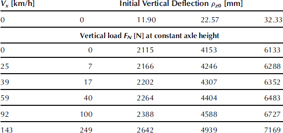
Pendulum and Yaw Oscillation Test Rigs
To assess the lateral and yaw tire dynamic parameters, two test rigs have been developed. One is the trailing arm ‘pendulum’ test stand with at one end a vertical hinge and at the other the steering head with a piezoelectric measuring hub. At that point the arm is excited laterally up to ca. 25 Hz through a hydraulic actuator, cf. Figure 9.38, and for more details: Chapter 12, Figure 12.8. The rig is useful to assess the overall relaxation length and the gyroscopic couple coefficient, both needed for the simpler transient models treated in Chapter 7. The idea of the pendulum concept originates from Bandel et al. (1989). They designed and used an actual pendulum rig. The natural frequency of the freely swinging trailing arm with a tire rolling on the drum was taken to establish the relaxation length σ. This quantity is the parameter of the first-order differential equation such as is used in Chapter 7. Bandel found that σ increases with speed. However, when using a model in which a belt ring with mass is used, it turns out that the parameters can be kept constant, cf. Vries and Pacejka (1998b). Consequently, tire inertia, notably the gyroscopic couples, gives rise to the speed dependency of the effective relaxation length.
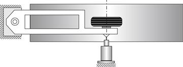
FIGURE 9.38 Principal sketch of the trailing arm ‘pendulum’ test rig exciting the tire almost purely laterally. Frequencies up to ca. 25 Hz, adequate for assessing the tire relaxation length and gyroscopic coupling parameter.
Another rig was developed to investigate the response of the tire subjected to yaw oscillations at frequencies up to ca. 65 Hz. The structure depicted in Figure 9.39 is light and very stiff; also see Figure 12.8. The two guiding members with flexible hinges intersect in the vertical virtual steering axis that is positioned in the wheel center plane (center point steering). A hydraulic actuator is mounted to generate the yaw vibration. The wheel axle is provided with a piezoelectric measuring hub. The tire is loaded by adjusting the axle height above the drum surface. During the test the loaded radius remains constant.
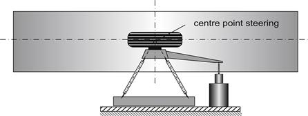
FIGURE 9.39 Principal sketch of the yaw oscillation test rig featuring center point steering. Frequencies up to ca. 65 Hz enabling the assessment of tire out-of-plane inertia and stiffness parameters including residual stiffnesses and rigid modes.
The measuring tower, cf. Figure 9.37, provided with a hydraulic vertical axle positioning installation is used to conduct pure braking and pure side slip tests as well as combined slip experiments at axle height oscillations and radial dynamic stiffness tests up to ca. 15 Hz.
A detailed description of the various side slip test facilities together with a full account of the numerous experiments conducted and the simulation results of the model have been given by Maurice (2000) and for motorcycle tires by Vries and Pacejka (1998a,b).
9.4.2 Dynamic Tire Simulation and Experimental Results
In general, the values of the model parameters can be estimated by minimizing the difference between measured and calculated frequency response functions (both amplitude and phase). In some cases (in particular the in-plane response), special aspects of the response functions may be considered to successfully assist the parameter assessment process. These aspects are: the position and width of resonance peaks (sidewall and residual stiffnesses and damping), the phase relationship in the low frequency range (overall relaxation length which itself is not a parameter!), and the yaw response at zero speed (yaw residual stiffness). The residual damping ratios have been chosen equal to those of the sidewalls. Another help is the establishment of the inertia parameters of the relevant part of the tire by cutting the tire into pieces and considering the parameters of these parts. Rolling over a cleat might be used to estimate some of the parameters but the most accurate way is the identification through frequency response functions. These are obtained with the aid of the random brake test with the measured brake torque (or the measured wheel speed) used as input, the yaw oscillation test, and the vertical axle oscillation test.
Vibrational Modes
The vibrational modes of the tire may be assessed through modal analysis of the tire wheel system with axle fixed and tire loaded and/or unloaded. When comparing these results with calculated modes using the parameter values assessed by means of the frequency response functions of the rolling tire, it is found that the stiffnesses found from the dynamic rolling experiments are ca. 30% lower than those estimated from experimental modal analysis, cf. Zegelaar. These differences must be due to the different operational conditions and the larger amplitudes of the vibrations and higher temperatures that occur in the realistic rolling experiments.
The calculated vibrational rigid body modes at zero speed using the parameters as established from experiments carried out on the drum have been depicted in Figures 9.40 and 9.41.
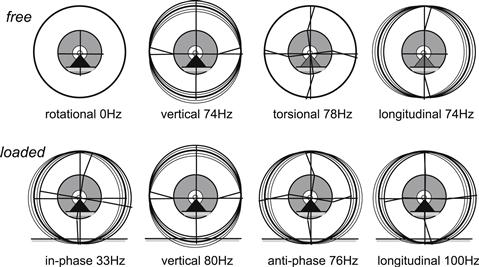
FIGURE 9.40 Calculated in-plane vibrational modes of tire/wheel system with axle fixed and tire free or loaded on the drum surface with vertical load FN = 4000 N and at zero speed.
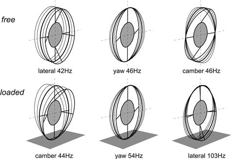
FIGURE 9.41 Calculated out-of-plane vibrational modes of tire/wheel system with axle fixed and tire free or loaded on the drum surface with vertical load FN = 4000 N and zero speed.
We have four in-plane degrees of freedom of the belt ring and the wheel rim (two translational and two rotational) and three out-of-plane degrees of freedom (lateral, yaw, and camber). As a consequence, we can distinguish four in-plane rigid modes and three out-of-plane rigid body modes. The mode shapes change considerably when the tire is making contact with the drum surface. The free rotation (0 Hz) mode changes into a mode with the belt and rim rotating in phase with respect to each other.
The lateral and camber modes appear to form combinations: one low frequency mode with a low axis of camber oscillations and one high frequency mode with a rotation axis closer to the top of the tire and relatively large lateral deflections in the contact zone. The yaw mode in the loaded case shows a higher calculated natural frequency since the effect of turn slip has been included, which was not the case in Maurice’s original model. This means that the yaw stiffness of the contact tread has now been accounted for.
The natural frequencies n and damping ratio ζ change with the speed of rolling. In Table 9.5 the values have been presented for the loaded tire running at a velocity of 0 and 30 m/s. Especially the out-of-plane modes show considerable changes in frequency and damping. The camber and yaw mode natural frequencies which are identical in the unloaded zero speed case, exhibit a with-speed growing mutual difference with the camber mode frequency becoming smaller and the yaw mode frequency larger.
TABLE 9.5 Natural Frequencies and Damping of Vibrational Modes of Rigid Ring Tire Model Calculated at a Vertical Load FN = 4000 N for Two Values of Forward Speed
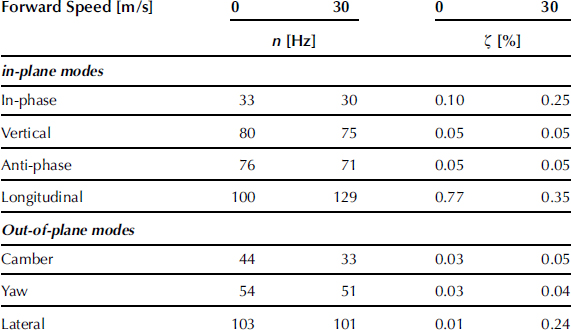
Frequency Response Functions
A typical example of measured and calculated in-plane frequency response functions has been depicted in Figure 9.42. Coherence functions show that the tests give sensible results up to ca. 80 Hz. Similar response functions have been obtained by Kobiki et al. (1990). The left-hand diagram of the figure represents the response function of the longitudinal force Fx (=Kaξ; in Eqn (9.195)) acting on the wheel axle to the imposed brake torque variation considered to be applied in the torque meter. The right-hand diagram shows the response of the force to wheel slip variations. The wheel slip is derived from the measured wheel and drum speeds.
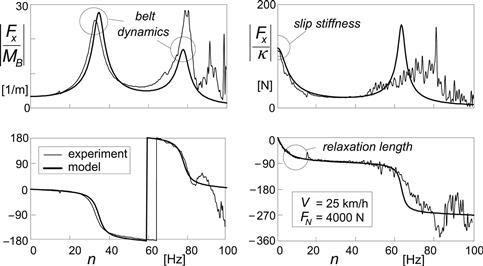
FIGURE 9.42 Measured and calculated in-plane frequency response functions at an average braking force of 450 N and assessed at a braking force standard deviation of 75 N.
The two peaks occurring in the left-hand diagram belong to the in-phase and the anti-phase modes. The single peak showing up in the right-hand diagram belongs to the mode that would arise if the rim were fixed also in rotation. The natural frequency lies in between the frequencies of the peaks in the left diagram. The natural frequencies contribute to assess the sidewall stiffnesses.
From the right-hand diagram two quantities can be derived: the slip stiffness and the overall relaxation length. Through the latter, additional information is obtained to find the fore-and-aft residual stiffness. From careful interpretation of the frequency response functions assessed at different speeds, the sidewall stiffness dependence on the speed of rolling has been ascertained. Resulting calculated response functions at different loads and brake torque level gave satisfactory agreement with measured behavior. We refer to the original work of Zegelaar (1998) for detailed information.
The out-of-plane frequency response functions of the side force Fy (=Kaη) and the aligning torque Mz (=Taζ) to yaw oscillations have been presented in Figures 9.43 and 9.44. The parameters have been assessed by minimizing the difference between measured and calculated (complex) response functions. The correspondence achieved between measured and computed curves at different speeds, loads, and side slip level is quite satisfactory; cf. Maurice (2000) for more details. To conduct a proper comparison, the measured data have been corrected for the inertia of the wheel and part of the tire that moves with the wheel.
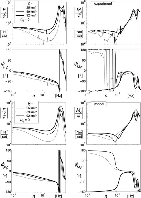
FIGURE 9.43 Measured and calculated out-of-plane frequency response functions of the side force and aligning torque to steer angle variations at zero average slip angle for three values of forward speed and normal load FN = 4000 N.
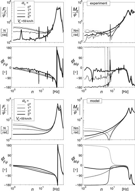
FIGURE 9.44 Measured and calculated out-of-plane frequency response functions of the side force and aligning torque to steer angle variations at one value of speed and at four levels of average side slip and wheel load FN = 4000 N.
The expected splitting up of the single peak at low velocity into two peaks, one belonging to the camber mode and the other to the yaw mode, and the growing difference of the two natural frequencies with increasing speed is clearly demonstrated. This phenomenon, which is due to gyroscopic action, has already been observed to occur with the stretched string model with inertia included approximately, cf. Figure 5.40. It is noted that the theoretical results of Maurice have been established by using the model that did not include the equations for the response to spin (9.177–9.180). Especially the aligning moment is sensitive to turn slip.
The moment response curves to side slip and yaw of the massless tire model as depicted in Figure 9.16 are quite different. The dip in the moment amplitude response curve to yaw oscillations occurring in the curve for Mψ in Figure 9.16 does not appear in the curve for the response to side slip Mα. This dip also appears in the curves of Figure 5.40 where spin is included as well. It is surprising to see that a similar dip occurs in Figures 9.43 and 9.44. The minimum arises here due to the tendency of the response to side slip to decrease and tend to zero at increasing path frequency while at the same time the moment amplitude increases due to tire inertia when approaching the resonance peak. The dip in the measured curve of the upper right-hand diagram of Figure 9.43 at 25 km/h is deeper than the one shown by the theoretical curve of the lower diagram. This may be due to the additional action of spin in the actual tire. As shown by both the theoretical and measured curves of Figure 9.44, the dip disappears altogether at larger average side slip.
The experiments conducted with the trailing arm ‘pendulum’ test rig, where the tire is subjected to almost pure side slip and the spin is very small, also show satisfactory correspondence with model behavior (Maurice 2000; also: De Vries and Pacejka, motorcycle tires, 1998b). This also appears to hold for a limited number of conducted combined slip tests and the response to vertical axle motions at side slip and braking carried out with the measuring tower.
Apparently, the rigid ring model provided with the short wavelength transient slip model is very well capable of describing the dynamic tire behavior in the frequency range up to about 60 Hz. Furthermore, it may be concluded that the spin part is only necessary when dealing with short wavelength, especially low-speed phenomena where tire inertia is less important, such as with parking.
Time Domain Responses
To demonstrate the performance of the model, simulations and experiments have been carried out pertaining to successive stepwise increases in brake pressure and steer angle.
The response of the longitudinal force and the associated wheel speed has been presented in Figure 9.45. The lower diagram clearly depicts the oscillatory variation of the force vs slip ratio. The measured response shows a faster decay of the wheel velocity after the highest brake effort has been reached. Apparently, this is due to the friction coefficient being lower in the experiment than assumed in the model. Finally, the brake is released and the wheel spins up again. The oscillations (ca. 28 Hz) correspond to the in-phase vibrational mode of the system, with the brake disc/axle inertia included.
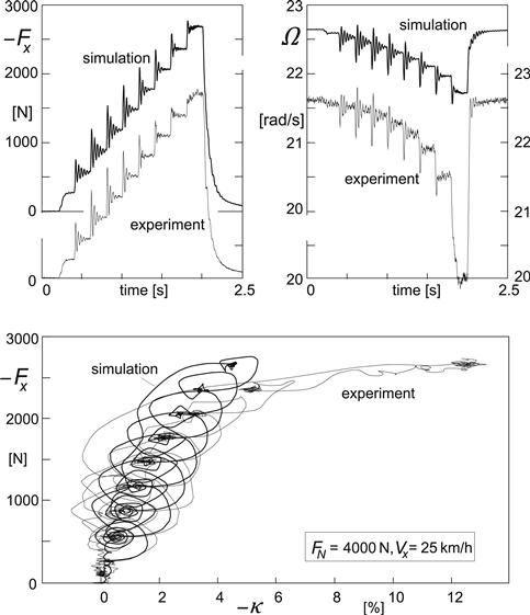
FIGURE 9.45 Brake force response to successive step increments of brake pressure. The upper diagrams depict the variation of force and wheel speed of revolution with time. The lower figure shows the loops in the force vs wheel slip diagram. Apparently, the actual friction coefficient is lower than assumed in the model. (Zegelaar 1998).
Figure 9.46 shows the responses to successive changes in steer angle for both the side force and the aligning torque at a given load and speed. The responses clearly show vibrations attributed to the yaw/camber mode with natural frequency of ca. 40 Hz (cf. Figure 9.43, 25 km/h). Also, the decrease of the overall relaxation length at larger slip angle can be recognized.
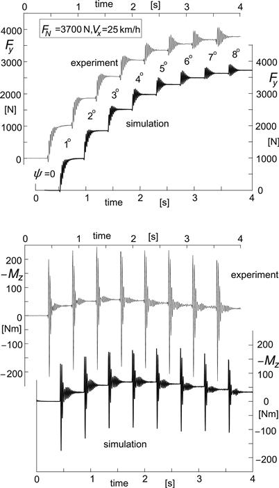
FIGURE 9.46 Side force and aligning torque response to successive step changes in steer angle. (Maurice 2000).