
Answers
Chapter 1: Recognition and Learning by a Computer
1.1. Recognition by a computer means the ability of a computer to recognize the pattern of an object that it already knows, and it can be looked at as a process of transforming the pattern function of an object into a more structured representation of the information. Recognition on a computer is about low-level information processing that can extract the structure of a pattern and high-level information processing that can understand conceptually the structure of a pattern structure using knowledge. On the other hand, in everyday life, the word recognition is used to mean knowing, conceptually understanding, finding true properties of an object, and so on.
1.2. Learning by a computer means that a system automatically generates either new data or a new program from its current state which will change the future output of the system so that some goal is achieved over a certain period of time. Finding the structure of information that is buried in a mass of information within a fixed time frame is also an important aspect of learning on a computer. In everyday life, learning means simply memorizing, understanding, explaining, acting on information, and so on.
1.3. Both recognition and learning by a computer can be looked at as the process of generating a new information that did not exist in the system before and transforming one representation to another. However, while recognition on a computer transforms representations starting from the pattern function representation of an object and, as a result, can generate a representation that is the same as the one that already exists in the system, learning on a computer does not have any constraints on the initial representation and generates a new representation that has not existed in the system before.
1.4. If we change the value of the right side of the expression (a) to −8, only one point satisfies the inequalities (a)-(c) and this point is x = 4, y = 4.
Chapter 2: Representing Information
2.1. We will show a program written in Pascal and its execution in Answer Figure 2.1.
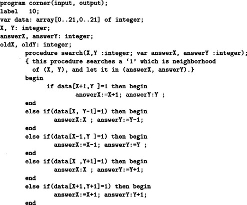
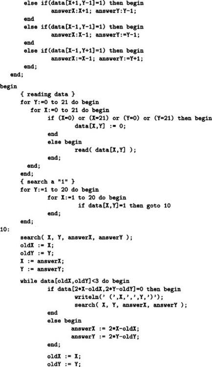
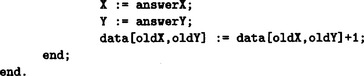
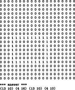
Answer Figure 2.1
2.2. (We will show an outline of the proof using mathematical induction.) When |N| = 1, it is true since |E| = 0. Now let us assume that it is true for |N| − 1(|N| ≤ 2) and prove that it is true for |N|. If |N| ≥ 2, find a k ∈ N that has only one branch of the form of (j, k). The graph that is obtained by removing this k from the tree, G′ = (N′, E′) (provided N′ = N − {k}, E′ = E − (j, k)), is a tree with only |N| − 1 nodes. Therefore, by induction, |E′| = |E′| − 1 is true for G′. But, |N′| = |N| − 1, |E′| = |E| − 1, so |E| = |E| − 1.
| input: | the list of branches D = (· · · (ni nj) · · ·), the initial node no, and the final node nd. |
| output: | the shortest path from n0 to nd represented as a list of nodes H, the length of the shortest path (the sum of the weights of the branches; in this problem this is equal to the number of branches) h. If there is no path from n0 to nd, output this fact. |
[1] Let h = 0, searched = {n0}, H = (n0), i = n0.
[2] If nd ∈ Searched, then stop. Output H, h.
[3] If there does not exist a node j where (i j) ∈ D and j ≠ searched, go to [6].
[4] If (i nd) ∈ D, then stop. Let h = h + 1 and H be the new list with nd added as the last element of H. Output H and h.
[5] Pick one node j where (i j) ∈ D and j ≠ Searched. Let h = h + 1 and Searched = Searched ∪ {j}. Let H be the list where j is added as the last element of H. Let i = j and go to [3].
[6] Let H be the list H with its last element removed. If ![]() , stop. Output the message that a route from n0 to nd does not exist. Otherwise, let i be the last element of H and go to [3].
, stop. Output the message that a route from n0 to nd does not exist. Otherwise, let i be the last element of H and go to [3].
This algorithm is not the logically best algorithm (it is based on the depth-first search method described in Section 3.6). There are many applications for the shortest path search and many algorithms are being studied to make the computation time shorter.
2.4. In Lisp, we can use a function reverse. For example,
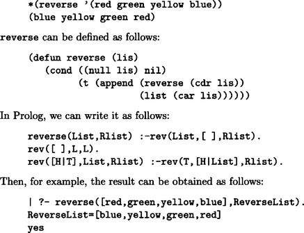
Lisp and Prolog are programming languages suited for transforming symbolic representations.
(a) (weather state raining)⇒(*wear raincoat)(*put-up umbrella)
(b) (electric_lightstateoff)(*electric_switchstateon)⇒(*check filament)
(c) (electric_light state off)(*electric_switchstateon)(filament state ok) ⇒ (*check fuse)
In an actual problem we would need to define each condition, the structure of sentences, and the semantic structure of actions. Here we showed examples only of what to write.
(a) isa: network example including multiple inheritance (Answer Figure 2.7.1)

Answer Figure 2.7.1
(b) A network example including both isa: and partof: (Answer Figure 2.7.2)
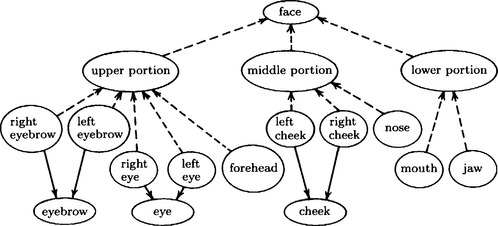
Answer Figure 2.7.2
Chapter 3: Generation and Transformation of Representations
3.1. If we let ![]() , then
, then ![]() . From this and (3.7), (3.8), and (3.9), we obtain
. From this and (3.7), (3.8), and (3.9), we obtain
If we generalize these to two dimensions, we obtain (3.10) and (3.11).
Therefore
and
3.3. For the Lagrange function
the solution to
is ![]() . Therefore,
. Therefore, ![]() is a local minimum of the original problem. On the other hand, if the goal function of the original problem is a convex function, then the local minimum becomes the global minimum. So,
is a local minimum of the original problem. On the other hand, if the goal function of the original problem is a convex function, then the local minimum becomes the global minimum. So, ![]() is the global minimum.
is the global minimum.
| input: | The list E of the edges of the weighted directed graph G and the list V of the nodes of G. |
| output: | The list M of the edges of the minimum spanning tree of G. |
[1] Generate the list D that sorts all the branches of G in order of increasing weight.
[3] If |M| < |V| − 1, remove the first element of D (vi, vj) ∈ E from D and go to [4]. Otherwise, stop. Output M.
[4] If the subgraph of G that consists of the branches of M ∪ {(vi, vj)} does not include a loop, let M = M ∪ {(vi, vj)} and go to [3].
This is not the fastest algorithm for obtaining the minimum spanning tree, because step [1] can be slow. There are other methods of obtaining the minimum spanning tree faster.
the set of axioms can be written
If we use ~cpu(m68386, Z) as a goal, we get Z = bonyson by the refutation process shown in Answer Figure 3.5.
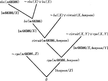
Answer Figure 3.5
3.6. If we thread the first list in working memory through the root node, node0 of the discrimination tree, it will go through node1, node2, node3, and finally reach node4, where the values of the variables $x, $y both become monkey. If we thread the second list through node0, it goes through node5, node6, node7, and node8, and reaches node9. In this case, the value of the variable $x becomes monkey. Now, since the assignment of the value to $x was not contradictory, the thread will extend to node10. Therefore, we can see that rule p1 is executable. On the other hand, since the list cannot be extended from node8 to node11, and therefore it cannot reach node12, rule p2 is not executable. In this case we see that only one rule, p1, is executable, and competition among the rules does not occur. If we execute p1, the working memory can be rewritten as
where bipedal(X) is thought of as a one variable function. In this way we can represent the simple slot-filler relation of frames using predicate logic. Also, for property inheritance in the frame representation, the properties of the more general frame can be copied into the less general frame beforehand, as long as the property to be inherited does not contain any contradictions. Therefore, inference in the frame representation about simple slot filling is logically equivalent to using a predicate logic representation. How ever, sometimes it is hard to represent information with heuristic meaning such as possibilities and the relation of cause and effect in predicate logic. For example, we can represent “if you are rich, you can buy a mansion” and “if you are rich, you can buy your own jet” using frames as follows:
In predicate logic, we can represent them as
In this case, we cannot infer “if you are rich, you can buy both a mansion and your own jet” from (1); however, by using the predicate logic inference rule
we can infer it from (2). In the first case you can buy either a mansion or your own jet, but it does not mean that you can buy both. This is the only case where we know the meaning of inference using the frame representation when we translate frames into predicate logic.
Chapter 4: Pattern Feature Extraction
4.1. Let f(x, y) be the sampling function at the mn points x = 0, 1,…, m − 1, y = 0, 1,…, n − 1. Then
First, computing ![]() requires 6mn multiplications and mn exponentiations. (There are two instances of (x − a)2 + (y − b)2, but they are each computed only once.) Therefore, to obtain k(x, y) for mn points (x, y), we require 6m2n2 multiplications and m2n2 exponentiations. Suppose m = n = 1000. Then, multiplication will be done 6 × 10¹² times and exponentiation will be done 1012 times. If, roughly speaking, one exponentiation takes 10 times as long as a multiplication, the computation will take 16 × 1012 the time of one multiplication. If we assume that one multiplication takes a microsecond, it will take more than 185 days to do this computation.
requires 6mn multiplications and mn exponentiations. (There are two instances of (x − a)2 + (y − b)2, but they are each computed only once.) Therefore, to obtain k(x, y) for mn points (x, y), we require 6m2n2 multiplications and m2n2 exponentiations. Suppose m = n = 1000. Then, multiplication will be done 6 × 10¹² times and exponentiation will be done 1012 times. If, roughly speaking, one exponentiation takes 10 times as long as a multiplication, the computation will take 16 × 1012 the time of one multiplication. If we assume that one multiplication takes a microsecond, it will take more than 185 days to do this computation.
This is a rough estimate, and there are methods for speeding up the computation. However, it should clear from this example that processing patterns requires a very high speed computer.
4.2. For each point of p,…, p5,
Using the coordinates (r, θ), we obtain the point of intersection of the above expressions. For example, for (2) and (3), from (3) – (2), the point of intersection is (r, θ) = (−4cos((tan−1(−2) ± nπ) ± mπ), tan−1(−2) ± nπ)(m, n = 0, ± 1,…). For (1) and (2), from (2) – (1), sinθ = 0. So, the point of intersection is given by (± ![]() , nπ) (n = 0, ± 1,…). The point X in Answer Figure 4.2 is the point of intersection of (1) and (2). In this case, since the x coordinates of the points p1 and p2 are the same, the point of intersection cannot be found by the method described in Section 4.2(c). (1)-(5) can be illustrated as in Answer Figure 4.2. In this figure, A′ and B′ are the highest points of intersection and they correspond to the straight line through p1, p3, and p4 and the straight line though p2, p3, and p5, respectively, which are shown by the broken lines in Figure 4.7(a).
, nπ) (n = 0, ± 1,…). The point X in Answer Figure 4.2 is the point of intersection of (1) and (2). In this case, since the x coordinates of the points p1 and p2 are the same, the point of intersection cannot be found by the method described in Section 4.2(c). (1)-(5) can be illustrated as in Answer Figure 4.2. In this figure, A′ and B′ are the highest points of intersection and they correspond to the straight line through p1, p3, and p4 and the straight line though p2, p3, and p5, respectively, which are shown by the broken lines in Figure 4.7(a).
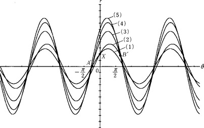
Answer Figure 4.2
[1] Let S be the given region.
[2] Execute the following steps for all the pattern elements s on the boundary line of S (those whose value is 1).
[2.1] If none of the pattern elements neighboring s are in the interior of the region (a pattern is in the interior of a region if it is within the region but not on the boundary), leave s as it is.
[3] Let S be the resulting region and go to [2].
In the above skeletonization algorithm, the skeletal representation of a square, for example, is only the center point. In order to avoid this, when the pattern element s in [2] is the end point of a boundary line, we can leave the value of s to be 1 without doing steps [2.1] and [2.2]. In this way, in the case of the square, the skeletal representation becomes the narrow region along the two diagonal lines of the square.
Another method of skeletonization and linear skeletonization is a method of shaving a pattern using the rule of local linear skeletonization by shifting an n x n (n = 3, 5, and so on) window in a fixed direction.
4.4. The wire frame representation is, as shown in the example of Figure 4.18, a spatial representation using the coordinates of the extreme points of the object, and it can represent solid and plane figures. On the other hand, a representation using the winged-edge model method, as shown in Figure 4.19, consists of the symbolic relation structure that represents the relation among the parts of an object and its features, and it can represent the general structure and features of solids and plane figures. Therefore, if we combine the wire frame representation and the winged-edge method, we can uniformly represent the spatial location, the structural relations, features, etc. of the parts of solids and plane figures.
Chapter 5: Pattern Understanding Methods
5.1. We can extract edges and regions by feature extraction; however, we cannot find out what the object is, what its features are, or what kinds of relations hold among several objects. In order to find this out, we need knowledge about the knowledge. We might need the following kinds of knowledge about an object: the name of the class it belong to, its spatial structure, its features, the relation between its local features and those of the class it belong to, a procedure for matching patterns with this knowledge, heuristic knowledge for finding features, knowledge about resolving contradictions between extracted features, knowledge for generating plans, inference procedures for using knowledge, and so on.
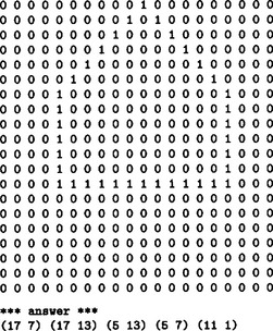
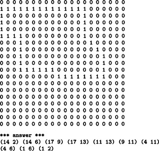
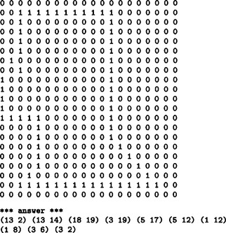
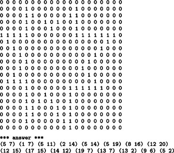
| input: | Two graphs, G1(V, E1), G2 = (V2, E2) (where V1 = V2 = {1,…,m}). |
| output: | A message stating whether they are graph isomorphic or not. |
5.3. In order to decide if an object (for example, a car) appears somewhere in a photograph (for example, a photograph of a road), we should divide the pattern into several subpatterns and try pattern understanding on each subpattern. Here the problem reduces to establishing a simple OR goal, and if a system can execute many pattern understanding routines in parallel, high execution speed is possible. For algorithms that generate plans including both OR goals and AND goals, please see Knowledge and Inference (Nagao (1990)).
Chapter 6: Learning Concepts
6.1. As we said in Section 6.2(a), we need to decide on what learning algorithm to use, how to use background information, the set of instances and a method of inputting them, and the representation of both instances and concepts. These are strongly related. For example, if we use predicate logic as the method of representation, then we can use the deductive transformations. If we use list representation, we would use algorithms for pattern matching. Also, if the set of instances includes noise, in other words, when it is possible that a positive (negative) example is interpreted as a negative (positive) example, we cannot usually make use of the methods described in this chapter. We will describe a method for dealing with noise in Chapter 9.
If we consider the conjunction to be the same as the set, ![]() , then, by Definition 5, pθ1, pθ2 is a positive example of p″η″. Also, there is no substitution ξ1″ for replacing the variable symbols of p″η″ with constant symbols that satisfies
, then, by Definition 5, pθ1, pθ2 is a positive example of p″η″. Also, there is no substitution ξ1″ for replacing the variable symbols of p″η″ with constant symbols that satisfies ![]() . Therefore, by Definition 5, pξ1 is a negative example of p″η″.
. Therefore, by Definition 5, pξ1 is a negative example of p″η″.
the following is a generalization of p1 and p2:

and there are no generalization p′ and substitution ξ1, ρi (i = 1,2) that make p ⊆ piξi,pi,p′ ⊆ piξi, p⊆p′pi (i = 1,2). So, by Definition 10, p is the MSC generalization of {p1, p2}. The following is the generalization that is not the MSC generalization:
with q = p1θ1 = p2η2, where
In this case, for the p given above, the substitutions θ1 and θ2, and
![]() so q is not the MSC generalization of p1
so q is not the MSC generalization of p1
Also, in the MSC generalization p, the constant symbols low and medium are replaced by the generalized variable symbol X, if we assume X ∈ {low, medium, high), then p becomes an overgeneralization. In order to prevent this, we should, for example, consider a representation that uses the disjunction medium ∨ low as the generalization. Unfortunately, if we allow this kind of representation, everything becomes very complicated.
6.4. Depending on the form of the functions u and v, integration by parts
can be easy to apply or hard to apply. For example, ∫ 3x cos x dx can be reduced to 3(x ∈ x + cos x) + c (c is a constant) by integration by parts if we let u = 3x and dv = cos x dx. Now, suppose that the positive example (where integration by parts can be applied easily)
is a maximal example, and the integration by parts for the general function
is a minimal example. Consider the version space shown in Answer Figure 6.4 and search the problem space where integration by parts can be applied easily in this space. For example, suppose
is presented as a positive example and
is presented as a negative example. By the former, the part of Answer Figure 6.4 including and below the circled node is left in the version space. By the latter, the part including and below the boxed nodes is removed from the version space. By repeating this operation, we can narrow down the problems that are easy to do by integration by parts. In order to find the circled nodes and the boxed nodes, we make use of the background knowledge that sin x and cos x are examples of trigonometric functions.
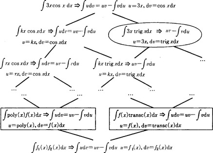
Answer Figure 6.4 Version space for integration by parts (Mitchell et al, 1983).
The above example is from Mitchell et al (1983).
Chapter 7: Learning Procedures
7.1. In the original problem, we would start from the initial state s0 of Section 7.1(a) (Figure 7.1); however, to simplify we consider here the goal state reached by solving the problem of Section 7.1(a) as the initial.
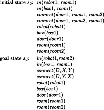
Now if we let g = {in(robot1, room2)}, we have g = a1θ for the add list of walkto a1 and the substitution θ = {robot1R, room2/Y}. So we rewrite
From this we prove so ![]() g and the substitution we get during the refutation process is ξ = {room1/X, door1/W}. Therefore, s0 can be changed to Sd by the operator
g and the substitution we get during the refutation process is ξ = {room1/X, door1/W}. Therefore, s0 can be changed to Sd by the operator
7.2. In the original problem we should start from the initial state so of Section 7.1(a) (Figure 7.1); however, to simplify, we generalize only the part of the problem dealt with in Problem 7.1. First, the triangular table for the answer to Exercise 7.1 is as shown in Answer Figure 7.2.1.
Answer Figure 7.2.1
The above triangular table can be generalized as shown in Answer Figure 7.2.2.
Answer Figure 7.2.2
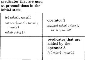
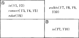
Using the above triangular table, we do the proof again. In other words, prove B using the precondition A and the precondition for the operator 3. The proof process is shown in Answer Figure 7.2.3.
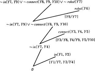
Answer Figure 7.2.3
If we do the substitution obtained from the triangular table, we obtain the generalized operator
This represents that “the robot Y6 moves by walking from room Y2 to Y5 through the door Y3.”
7.3. The sample program written in Lisp is shown in Answer Figure 7.3. To run this program, we setq the list of rules to the atom productions and the list containing the working memories to the atom wms, and evaluate the function start. The rule for generating and adding a new rule to the set of rules,
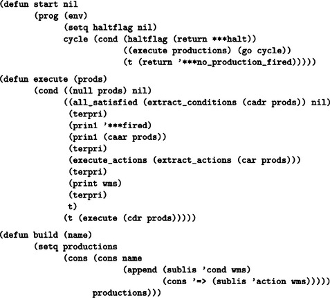
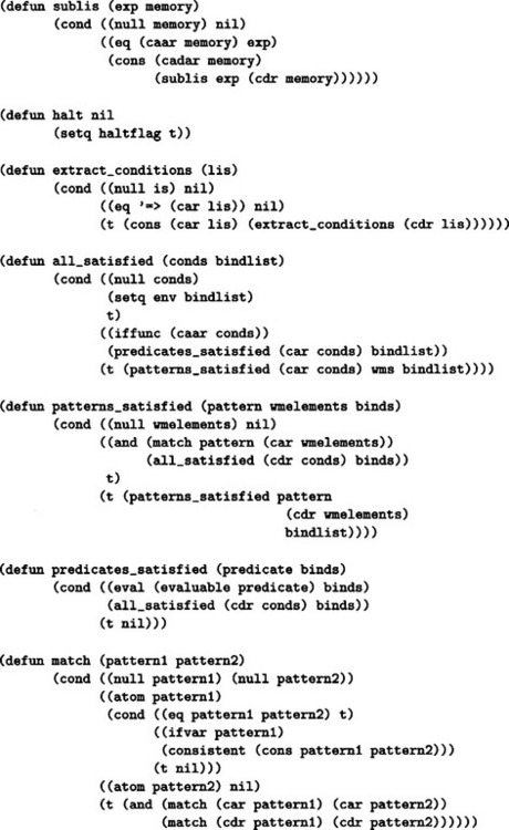
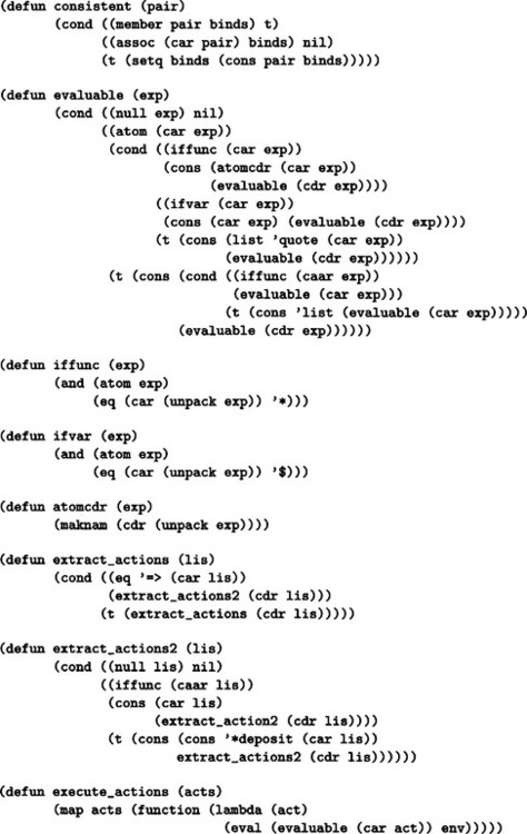
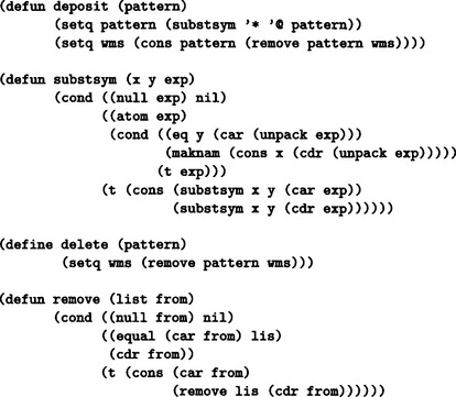
Answer Figure 7.3
should be placed in front of the initial set of the rules. If there is no function in the head of the action, we omit *deposit (adding the value of the argument to the head of the working memory). Also, the lists maintained in working memory that are candidates for conditions or actions should be in the form (cond <condition>) and (action <action>), respectively. For a function with © instead of * in the head of an <action>, © is changed to * when such a function is entered into the working memory. For example, if (action (©deposit (a b c))) is executed as the action of a rule, (action (*deposit (a b c))) is added to the front of the working memory. In this program, if at least one list with cond and action as its head exists in working memory, the program executes the rule rg, it generates a new rule (within working memory) consisting of all the lists whose head is cond or action, and it adds such a rule to the front of the set of rules. Then it deletes the used lists from working memory. By the way, the atoms with * as their head on the action side are all evaluated as functions. In particular, to stop the execution of the rule, we can let the action side execute the a rule including (*halt) which evaluates the function halt.
7.4. In the course of problem solving described in Exercise 7.3, (clear a) caused a loop on the state. For this reason we might put this subgoal at the beginning and change the order of subgoals in the original goal. As a result, we can solve the problem as follows:
This is an example of a case where we can solve a problem by changing the order of the subgoals in different classes or the subgoals in the same class.
Unfortunately, it is not so easy to introduce this operation into procedural learning as described in Section 7.3 and to build a system for learning how to change the structure of a subgoal.
Chapter 8: Learning Based on Logic
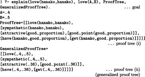
The following Horn clause is a sufficient condition:
![]()
The above well-formed formula can be interpreted as “a person who has good points and who is sympathetic to other people loves other people.” This is an overgeneralization of the positive example
![]()
This is due to the fact that the background information is too general.
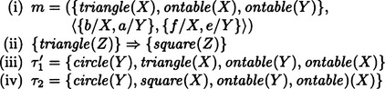
8.3. The knowledge that a swallow, a sparrow, a robin, and a hawk are birds can be represented by the following well-formed formula:
To say that only swallows, sparrows, robins, and hawks are birds, we use the following well-formed formula:
Consider the inference rule
(where p(X), q(X) correspond to (i) and (ii), respectively). Next, to generalize (iii), consider the following inference rule for an arbitrary well-formed formula r(X) and an arbitrary predicate w(X):
where P is a well-formed formula that can be proved from P(w). Since (iv) includes P(r), it is an inference rule of second-order predicate logic and the basic inference rule in circumscription. In this problem, we can assume, for example, the following:
(where P(w), in other words, (∀X)(bird(X) → canfly(X)) is true). From this we can conclude that if Y is a bird, then Y must be either a swallow, a sparrow, a robin, or a hawk.
Chapter 9: Learning by Classification and Discovery
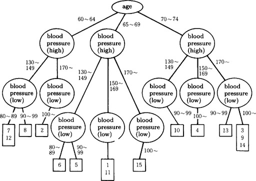
9.1. One example of a discrimination tree is shown in Answer Figure 9.1. (It does not include the classification of +-.)
Answer Figure 9.1
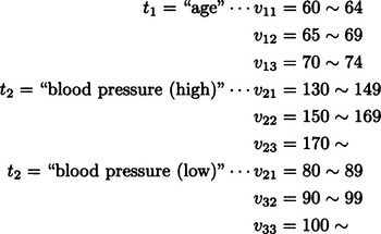
9.2. Similar to the answer to Exercise 9.1, we look at the value of each attribute classified as follows (the symbols are those of Section 9.3):
If we call the number of data points classified as +, −, d1 and d2, respectively, we have d1 = 6, d2 = 9. Also,
Furthermore,
Clearly
Therefore
and maxj G(tj) can be obtained by t2 = “blood pressure(high).” Now, if we choose “blood pressure(high)” as a test in the root node of the discrimination tree, we can maximize the amount of information. Actually, in this example, since E′(blood pressure(high)) = 0, the amount of information in the discrimination tree as a whole and the amount of information when we chose “blood pressure (high)” as the first test are the same. This means that the test of “blood pressure(high)” alone can classify the data into two classes of +, −.
we let X0 = {m, v, E}. If we set the initial state to X0 and do breadth-first search using the operators o, / that are defined in Definition 2 in Section 9.5(a), we obtain the constant vector m ![]() v
v ![]() v/E = (2,2,2,2,2,2). (If we generalize this, we can obtain E =
v/E = (2,2,2,2,2,2). (If we generalize this, we can obtain E = ![]() mv2, in other words, the expressions of the relation between the speed of an object and energy in Newtonian dynamics.) Answer Figure 9.3 shows part of the search tree.
mv2, in other words, the expressions of the relation between the speed of an object and energy in Newtonian dynamics.) Answer Figure 9.3 shows part of the search tree.
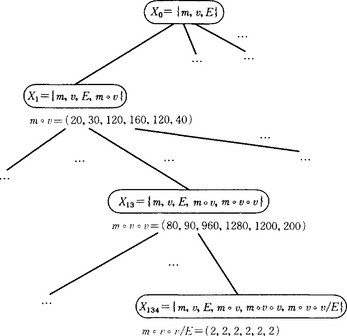
Answer Figure 9.3
Chapter 10: Learning by neural networks
| back propagation error learning | competitive learning | |
| structure of the neural network | feedforward network | feedforward cluster |
| learning method | supervised learning | unsupervised learning |
| learning rule for net weight | generalization delta rule | intensification based on conflict |
| Hopfield network | Boltzmann machine | |
| behavior of corollary | deterministic | probabilistic |
| value the state can take | [0, 1] | {0,1} |
| state transition | deterministic | probabilistic |
10.2. [4], [5], [6] show that an output unit and the units in its neighborhood where the corresponding input vector is closest to the unit’s weight are selected and the weights of the links that combine such units are reactivated. By repeating this operation, the unit weight that represents the distribution of the input vector in some sense is created in several output units. In other words, we can divide the set of the input vector into several clusters by vector quantization.
10.3. The following is a partial list of the necessary functions:
(1) macro commands for simply defining many units and links.
(2) a template for modulizing the computation at each layer and cluster.
(3) commands for making simple definitions of output functions, state transition functions, and so on.
(4) functions for uniform random numbers, probabilistic distribution functions, and so on.
(5) input functions for reading masses of input data and for managing data bases.
(6) descriptions of functions that change the values of the energy function, the unit weights, the states, and so on.
(7) human/machine interface for showing clearly the structure of the network, and so on.