Congestion Control in High-Speed Networks
This chapter discusses congestion control in high-speed networks with long latencies. One of the consequences of the application of control theory to TCP congestion control was the realization that TCP Reno was inherently unstable as the delay-bandwidth product of the network became large or even for very large bandwidths. As a result of this, a number of new congestion control designs were suggested with the objective of solving this problem such as High-Speed TCP (HSTCP), TCP Binary Increase Congestion control (BIC), TCP CUBIC, and Compound TCP (CTCP), which are described in this chapter. Currently, TCP CUBIC serves as the default congestion control algorithm for Linux servers and as a result is as widely deployed as TCP Reno. CTCP is used as the default option for Windows servers and is also very widely deployed. We also describe the eXpress Control Protocol (XCP) and Rate Control Protocol (RCP) algorithms that have been very influential in the design of high-speed congestion control protocols. Finally, we make connections between the algorithms in this chapter and the stability theory from Chapter 3 and give some general guidelines to be used in the design of high-speed congestion control algorithms.
Keywords
Congestion control in high-speed networks; TCP over high-speed links; TCP Response Function; HSTCP; High-Speed TCP; TCP BIC; TCP CUBIC; CTCP; Compound TCP; FAST TCP; XCP Congestion Control; RCP Congestion Control; Scalable TCP; Yeah-TCP; TCP Africa; TCP Illinois
5.1 Introduction
Link speeds have exploded in the past 2 decades from tens of megabits to multiple gigabits per second for both local as well as long-distance networks. The original congestion control algorithms for TCP, such as Reno and Tahoe, worked very well as long as the link speeds were lower but did not scale very well to the higher speeds and longer propagation delays for several reasons:
• In Chapter 3, Section 3.4, by using a control theory framework, it was shown that TCP Reno becomes unstable if either the link capacity, the propagation delay, or both become large. This results in severe oscillations of the transmission rates and buffer occupancies, which has been observed in practice in high-speed networks.
• Consider the following scenario: The link capacity is 10 Gbps, and the Round Trip Latency (RTT) is 100 ms, so the delay bandwidth product is about 100,000 packets (for a packet size of 1250 bytes). For TCP to grow its window from the midpoint (after a multiplicative decrease) to full window size during the congestion avoidance phase, it will require 50,000 RTTs, which is about 5000 seconds (1.4 hours). If a connection finishes before then, the link will be severely underutilized. Hence, when we encounter a combination of high capacity and large end-to-end delay, the multiplicative decrease policy on packet loss is too drastic, and the linear increase is not quick enough.
• The square-root formula for TCP throughput (see Chapter 2) shows that for a round trip latency of T, the packet drop rate has to be less than 1.5(RT)2![]() to sustain an average throughput of R. Hence, using the same link and TCP parameters as above, the packet drop rate has to be less than 10−10
to sustain an average throughput of R. Hence, using the same link and TCP parameters as above, the packet drop rate has to be less than 10−10![]() to sustain a throughput of 10 Gbps. This is much smaller than the drop rate that can be supported by most links.
to sustain a throughput of 10 Gbps. This is much smaller than the drop rate that can be supported by most links.
A number of alternate congestion control algorithms for high-speed networks were suggested subsequently to solve this problem, including Binary Increase Congestion control (BIC) [1], CUBIC [2], High-Speed TCP (HSTCP) [3], ILLINOIS [4], Compound TCP (CTCP) [5], YEAH [6], and FAST TCP [7]. The Linux family of operating systems offers users a choice of one of these algorithms to use (in place of TCP Reno) while using TCP CUBIC as the default algorithm. The Windows family, on the other hand, offers a choice between Reno and CTCP. As a result of the wide usage of Linux on web servers, it has recently been estimated [8] that about 45% of the servers on the Internet use either BIC or CUBIC, about 30% still use TCP Reno, and another 20% use CTCP.
In this chapter, we provide a description and analysis of the most popular high-speed congestion control algorithms, namely HSTCP, BIC, CUBIC, and CTCP. Each of these algorithms modifies the TCP window increase and decrease rules in a way such that the system is able to make better utilization of high-speed and long-distance links. We also discuss two other protocols, namely eXpress Control Protocol (XCP) and Rate Control Protocol (RCP). These need multi-bit network feedback, which has prevented their deployment in Internet Protocol (IP) networks. However, several interesting aspects of their design have influenced subsequent protocol design. Whereas XCP and RCP approach the high-speed congestion control problem by using an advanced Active Queue Management (AQM) scheme, the other algorithms mentioned are server based and designed to work with regular tail-drop or Random Early Detection (RED) routers.
The rest of this chapter is organized as follows: Section 5.2 introduces the concept of the Response Function and its utility in designing and analyzing congestion control algorithms, Sections 5.3 to 5.8 discuss the design and analysis of a number of high-speed congestion control algorithms, including HSTCP (Section 5.3), TCP BIC (Section 5.4.1), TCP CUBIC (Section 5.4.2), Compound TCP (Section 5.5), FAST TCP (Section 5.6), XCP (Section 5.7), and RCP (Section 5.8). Section 5.9 contains some observations on the stability of these algorithms.
An initial reading of this chapter can be done in the sequence 5.1→5.2→5.3 followed by either 5.4 or 5.5 or 5.6 or 5.7 or 5.8 (depending on the particular algorithm the reader is interested in)→5.9.
5.2 Design Issues for High-Speed Protocols
In networks with large link capacities and propagation delays, the congestion control protocol needs to satisfy the following requirements:
1. It should be able to make efficient use of the high-speed link without requiring unrealistically low packet loss rates. As pointed out in the introduction, this is not the case for TCP Reno, because of its conservative window increase and aggressive window decrease rules.
2. In case of very high-speed links, the requirement of intraprotocol fairness between the high speed TCP protocol and regular TCP is relaxed because regular TCP is not able to make full use of the available bandwidth. Hence, in this situation, it is acceptable for the high speed TCP variants to perform more aggressively than standard TCP.
3. If connections with different round trip latencies share a link, then they should exhibit good intraprotocol fairness.
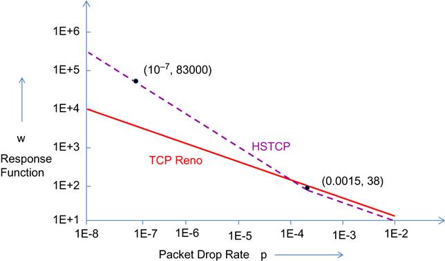
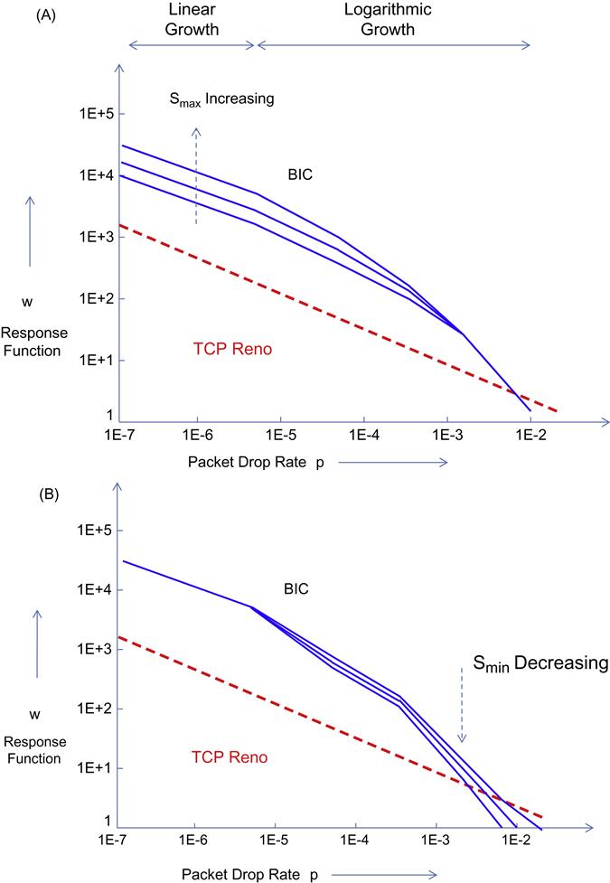
Define the Response Function w of a congestion control algorithm as w=Ravg.T packets per round trip time (ppr), where Ravg is the average throughput and T is the minimum round trip latency. This is sometimes also referred to as the average window because it is the average number of packets transmitted per round trip time. A basic tool used to evaluate high-speed designs is the log-log plot of the Response Function versus p (Figure 5.1). Note that the ability of a protocol to use the high amount of bandwidth available in high-speed networks is determined by whether it can sustain high sending rates under low loss rates. From Figure 5.1, it follows that a protocol becomes more scalable if its sending rate is higher under lower loss rates.
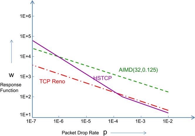
From Chapter 2, the Response Function for TCP Reno is given by
w=√32porlogw=0.09−0.5logp (1)
 (1)
(1)
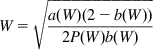
This plot is shown in Figure 5.1, along with the plot for the Response Function of some high-speed algorithms.
• Additive increase/multiplicative decrease AIMD(32, 0.125) corresponds to an AIMD algorithm (introduced in Section 2.3.1 of Chapter 2) with an additive increase of 32 packets and a multiplicative decrease factor of 0.125. From equation 72 in Chapter 2, the response function for AIMD(32, 0.125) is given by
logw=1.19−0.5logp (2)
Hence AIMD(32, 0.125) has the same slope as Reno on the log-log plot but is able to achieve a higher window size for both high- and lower link speeds.
• The HSTCP response function is derived in Section 2.3 (equation 8), and is given by
logw={−0.82−0.82logpifp<0.00150.09−0.5logpotherwise (3)
This response function coincides with that of Reno for larger values of the packet drop rate, but for smaller values, it exhibits a steeper slope, which explains its better performance in high-speed links.
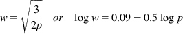
Even though Figure 5.1 plots the response function versus the packet drop rate, it also implies a relationship between the response function and the link capacity as we show next. We will consider the case when all packet drops are due to buffer overflows, so from equation 53 in Chapter 2, it follows that the number of packets N transmitted during a single cycle for TCP Reno is given by
N=3W2m8
where Wm is the maximum window size. But Wm≈CT![]() if we ignore the contribution caused by the buffer occupancy. Hence, it follows that the packet drop probability p is given by
if we ignore the contribution caused by the buffer occupancy. Hence, it follows that the packet drop probability p is given by
p=1N≈83W2m=83(CT)2
which implies that the packet drop probability is inversely proportional to the square of the link speed. This is also illustrated in Figure 5.2, which shows the frequency of packet drops decreasing as the window size increases for two connections that pass through links with different capacities but with the same round trip latency. Hence, it follows that small values of p correspond to a large link capacity and vice versa.
Note the following features for the graph in Figure 5.1:
1. At small values of p (or equivalently for very high-speed links), it is desirable that the Response Function for the high-speed protocol be much larger than for TCP Reno because this implies that for a given interval between packet drops (which is the inverse of the packet loss rate), the congestion window can grow to a much larger value compared with Reno. Note that this implies that if Reno and the high-speed protocol compete for bandwidth in a high-speed link, the latter will end up with a much larger portion of the bandwidth (i.e., the system will not be fair). However, this is deemed to be tolerable because the high-speed protocol is taking up link bandwidth that cannot be used by TCP Reno anyway.
2. At larger values of p (or equivalently lower speed links), it is desirable for TCP friendliness that the point at which the two curves cross over lie as much to the left as possible. The reason for this is that for lower speed links, the congestion control algorithm should be able to sustain smaller window sizes, which is better suited to coexisting with TCP Reno without taking away bandwidth from it. To do this, the Response Function for the high-speed algorithm should be equal to or lower than that for TCP Reno after the two curves cross over.
3. To investigate the third requirement regarding intraprotocol RTT fairness, we can make use of the following the result that was derived in Chapter 2:
Assume that the throughput of a loss based congestion control protocol with constants A, e, d is given by
R=ATepdpackets/s
Then the throughput ratio between two flows with round trip latencies T1 and T2, whose packet losses are synchronized, is given by
R1R2=(T2T1)e1−d (4)
Note that as d increases, the slope of the response function and RTT unfairness both increase (i.e., the slope of the response function on the log-log plot determines its RTT unfairness).
Thus, by examining the Response Function graph, one can verify whether the high-speed protocol satisfies all the three requirements mentioned.
To satisfy the first requirement, many high-speed algorithms use a more aggressive version of the Reno additive increase rule. Hence, instead of increasing the window size by one packet per round trip time, they increase it by multiple packets, and the increment size may also be a function of other factors such as the current window size or network congestion. However, to satisfy the second requirement of TCP friendliness, they modify the packet increase rule in one of several ways. For example:
• HSTCP [3] reverts to the TCP Reno packet increment rule when the window size is less than some threshold.
• Compound TCP [5] and TCP Africa [9] keep track of the connections’ queue backlog in the network and switch to a less aggressive packet increment rule when the backlog exceeds a threshold.
There is also a tradeoff between requirements 2 and 3 as follows: Even though it is possible to design a more TCP-friendly protocol by moving the point of intersection with the TCP curve to a lower packet drop rate (i.e., to the left in Figure 5.1), this leads to an increase in the slope of the Response Function line, thus hurting RTT fairness.
5.3 High Speed TCP (HSTCP) Protocol
HSTCP by Floyd et al. [3,10] was one of the first TCP variants designed specifically for high-capacity links with significant propagation delays. The design for HSTCP was based on the plot of the Response Function versus Packet Drop Rate introduced in the previous section and proceeds as follows: The ideal response function for a high-speed congestion control algorithm should have the following properties:
• The HSTCP Response Function should coincide with that of TCP Reno when the packet drop rate exceeds some threshold P (or equivalently when the congestion window is equal to or less than W packets). As a default HSTCP chooses P0=0.0015 and W0=38 packets.
• We next choose a large ppr, say, W1=83,000 packets (which corresponds to a link capacity of 10 Gbps for packet size of 1500 bytes and round trip time T=100 ms) and a corresponding packet loss rate of P1=10−7. For packet loss rates less than P0, we specify that the HSTCP Response Function should pass through the points (P0, W0) and (P1, W1) and should also be linear on a log-log scale (Figure 5.3).
As a result, the Response Function for HSTCP is given by
logw=S(logp−logP0)+logW0 (5)
where
S=logW1−logW0logP1−logP0 (6)
Equation 5 can be rewritten as
w=W0(pp0)Spackets (7)
If we substitute the values of (P0,W0) and (P1,W1) in equation 6, then we obtain S=−0.82, so that the HSTCP Response Function is given by
w=0.15p0.82packetsforp≤P0. (8)
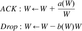
We now derive an expression for the AIMD increase–decrease parameters for HSTCP. The window size W in HSTCP uses the following AIMD rules with increase–decrease functions a(w) and b(w) that are functions of the window size (these are implemented on a per-ACK basis):
ACK:W←W+a(W)WDrop:W←W−b(W)W (9)
 (9)
(9)
For the case W≤W0![]() , HSTCP defaults to TCP Reno so that
, HSTCP defaults to TCP Reno so that
a(W)=1andb(W)=0.5forW≤W0. (10)
For W>W0, we assume that b(W) varies linearly with respect to log(W) for W∈[W0,W1]![]() With b(W0)=0.5 and b(W1)=B, where B is the target minimum value for B(w) for W=W1, (Floyd et al. [3] recommend a value of B=0.1 at W=W1), we obtain
With b(W0)=0.5 and b(W1)=B, where B is the target minimum value for B(w) for W=W1, (Floyd et al. [3] recommend a value of B=0.1 at W=W1), we obtain
b(W)=(B−0.5)logW−logW0logW1−logW0+0.5 (11)
To obtain the corresponding a(W), we use the following formula for the response function of AIMD congestion control (this was derived in Section 2.3.1 in Chapter 2). We choose a point W∈[W0,W1]![]() and compute the corresponding probability P(W) by using equation 5. Substitute (P(W),W) into the following equation
and compute the corresponding probability P(W) by using equation 5. Substitute (P(W),W) into the following equation
W=√a(W)(2−b(W))2P(W)b(W) (12)
 (12)
(12)
so that
a(W)=P(W)W22b(W)2−b(W) (13)
Note that there are a couple of heuristics in the use of equation 12: (1) equation 12 is a formula for the response time function, not the window size, and (2) equation 12 was derived for the case when a and b are constants, which is not the case here.
Table 5.1 gives the values of a(W) and b(W) using equations 11 and 13 for some representative values of W between 38 and 84,035.
Table 5.1
| W | a(W) | b(W) |
| 38 | 1 | 0.5 |
| 1058 | 8 | 0.33 |
| 10661 | 30 | 0.21 |
| 21013 | 42 | 0.17 |
| 30975 | 50 | 0.15 |
| 40808 | 56 | 0.14 |
| 51258 | 61 | 0.13 |
| 71617 | 68 | 0.11 |
| 84035 | 71 | 0.1 |
a(W), defined in equation (13); b(W), defined in equation (11); W, HSTCP Window Size.
Even though HSTCP is not widely used today, it was one of the first high-speed algorithms and served as a benchmark for follow-on designs that were done with the objective of addressing some of its shortcomings. A significant issue with HSTCP is the fact that the window increment function a(w) increases as w increases and exceeds more 70 for large values of w, as shown in Table 5.1. This implies that at the time when the link buffer approaches capacity, it is subject to a burst of more than 70 packets, all of which can then be dropped. Almost all follow-on high-speed designs reduce the window increase size as the link approaches saturation. HSTCP is more stable than TCP Reno at high speeds because it is less aggressive in reducing its window after a packet loss which reduces the queue size oscillations at the bottleneck node.
If we apply equation 4 to HSTCP, then substituting e=1, d=0.82, we obtain
R1R2=(T2T1)11−d=(T2T1)5.55 (14)
Hence, because of the aggressive window increment policy of HSTCP, combined with small values of the decrement multiplier, connections with a larger round trip latency are at a severe throughput disadvantage. There is a positive feedback loop which causes the connection with the large latency to loose throughput, which operates as follows: Even if the two connections start with the same window size, the connection with smaller latency will gain a small advantage after a few round trip delays because it is able to increase its window faster. However this causes its window size to increase, which further accelerates this trend. Conversely the window size of the large latency connection goes into a downward spiral as reductions in its throughput causes a further reduction in its window size.
5.4 TCP BIC and CUBIC
Both TCP BIC and CUBIC came from the High-Speed Networks Research Group at North Carolina State University [1,11]. TCP BIC was invented first and introduced the idea of binary search in congestion control algorithms, and TCP CUBIC was later designed to simplify the design of BIC and improve on some of its weaknesses. Both these protocols have been very successful, and currently TCP CUBIC serves as the default congestion control choice on the Linux operating system. It has been estimated [8] that TCP BIC is used by about 15% of the servers in the Internet, and CUBIC is used by about 30% of the servers.
The main idea behind TCP BIC and CUBIC, is to grow the TCP window quickly when the current window size is far from the link saturation point (at which the previous loss happened), and if it is close to the saturation point then the rate of increase is slowed down (see Figure 5.5 for BIC and Figure 5.8 for CUBIC). This results in a concave increase function, which decrements the rate of increase as the window size increases. The small increments result in a smaller number of packet losses if the window size exceeds the capacity. This makes BIC and CUBIC very stable and also very scalable. If the available link capacity has increased since the last loss, then both BIC and CUBIC increase the window size exponentially using a convex function. Since this function shows sub-linear increase initially, this also adds to the stability of the algorithm for cases in which the new link capacity did not increase significantly.
5.4.1 TCP BIC
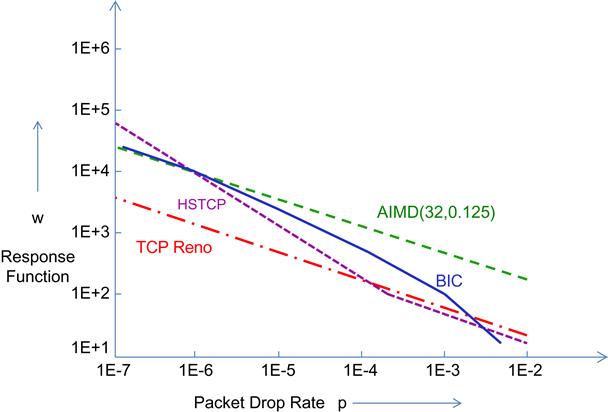
The objective of BIC’s design is to satisfy the three criteria of RTT fairness, TCP friendliness, and scalability. The algorithm results in a concave response time function for BIC as shown in Figure 5.4, from which we can observe the following:
• Because the BIC response time graph intersects with that of Reno around the same point as that of HSTCP, it follows BIC is also TCP friendly at lower link speeds.
• The slope of BIC’s response time at first rises steeply and then flattens out to that of TCP Reno for larger link speeds. This implies that for high-speed links, BIC exhibits the RTT fairness property.
• Because of the fast initial rise in its response time, BIC scales well with link speeds.
The evolution of BIC’s congestion window proceeds in three stages (Figure 5.5): additive increase, binary search increase, and max probing.
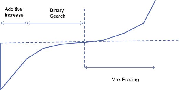
5.4.1.1 Binary Search Increase
The Binary Search window increase rule in BIC was inspired by the binary search algorithm and operates as follows:
• If Wmax is the maximum window size that was reached just before the last packet loss, and Wmin is the window size just after the packet loss, then after 1 RTT, the algorithm computes Wmid, the midpoint between Wmax and Wmin, and sets the current window size to Wmid.
• After the resulting packet transmissions:
• If there are no packet losses, then Wmin is set to Wmid, or
For the case of no packet losses the process repeats for every RTT until the difference between Wmax and Wmin falls below a preset threshold Smin. Note that as a result of this algorithm, the window size increases logarithmically.
Just as for binary search, this process allows the bandwidth probing to be more aggressive when the difference between the current window and the target window is large and gradually becomes less aggressive as the current window gets closer to the target. This results in a reduction in the number of lost packets as the saturation point is reached. This behavior contrasts with HSTCP, which increases its rate near the link saturation point, resulting in excessive packet loss.
5.4.1.2 Additive Increase
When the distance to Wmid from the current Wmin is too large, then increasing the window to that midpoint leads to a large burst of packets transmitted into the network, which can result in losses. In this situation, the window size is increased by a configured maximum step value Smax. This continues until the distance between Wmin and Wmid falls below Smax, at which the Wmin is set directly to Wmid. After a large window size reduction, the additive increase rule leads to an initial linear increase in window size followed by a logarithmic increase for the last few RTTs.
For large window sizes or equivalently for higher speed links, the BIC algorithm performs more as a pure additive increase algorithm because it spends most of its time in this mode. This implies that for high-speed links, its performance should be close to that of the AIMD algorithm, which is indeed the case from Figure 5.4.
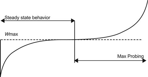
5.4.1.3 Max Probing
When the current window size grows past Wmax, the BIC algorithm switches to probing for the new maximum window, which is not known. It does so in a slow-start fashion by increasing its window size in the following sequence for each RTT: Wmax+Smin, Wmax+2Smin, Wmax+4Smin,…,Wmax+Smax. The reasoning behind this policy is that it is likely that the new saturation point is close to the old point; hence, it makes sense to initially gently probe for available bandwidth before going at full blast. After the max probing phase, BIC switches to additive increase using the parameter Smax.
BIC also has a feature called Fast Convergence that is designed to facilitate faster convergence between a flow holding a large amount of bandwidth and a second flow that is starting from scratch. It operates as follows: If the new Wmax for a flow is smaller than its previous value, then this is a sign of a downward trend. To facilitate the reduction of the flow’s bandwidth, the new Wmax is set to (Wmax+Wmin)/2, which has the effect of reducing the increase rate of the larger window and thus allows the smaller window to catch up.
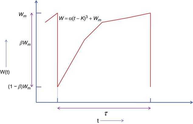
We now provide an approximate analysis of BIC using the sample path–based fluid approximation technique introduced in Section 2.3 of Chapter 2. This analysis explains the concave behavior of the BIC response time function as illustrated in Figure 5.4. We consider a typical cycle of window increase (see Figure 5.6), that is terminated when a packet is dropped at the end of the cycle.
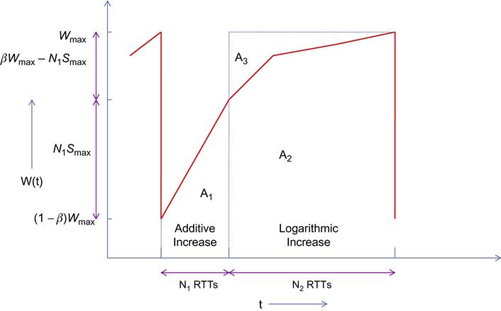
N1: Number of RTT rounds in the additive increase phase
N2: Number of RTT rounds in the logarithmic increase phase
Y1: Number of packets transmitted during the additive increase phase
Y2: Number of packets transmitted during the logarithmic increase phase
As per the deterministic approximation technique, we make the assumption that the number of packets sent in each cycle of the congestion window is fixed (and equal to 1/p, where p is the packet drop rate). The average throughput Ravg is then given by
Ravg=Y1+Y2T(N1+N2)=1/pT(N1+N2) (15)
We now proceed to compute the quantities Y1, Y2, N1 and N2.
Note that β![]() is multiplicative decrease factor after a packet loss, so that
is multiplicative decrease factor after a packet loss, so that
Wmin=(1−β)Wmax (16)
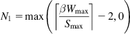
BIC switches to the logarithmic increase phase when the distance from the current window size to Wmax is less than 2Smax; hence, if this distance less than this, there is no additive increase. Because Wmax−Wmin=βWmax![]() , it follows that N1 is given by
, it follows that N1 is given by
N1=max(⌈βWmaxSmax⌉−2,0) (17)
 (17)
(17)and the total increase in window size during the logarithmic increase phase is given by βWmax−N1Smax![]() , which we denote by X. Note that
, which we denote by X. Note that
X2+X22+⋯+X2N2=X−Smin (18)
This equation follows from the fact that the X is reduced by half in each RTT of the logarithmic increase phase until the distance to Wmax becomes less than Smin. From equation 18, it follows that
X(1−12N2)=X−Smin,sothat
N2=log(βWmax−N1SmaxSmin)+2 (19)
Note that 2 has been added in equation 19 to account for the first and last round trip latencies of the binary search increase.
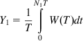
We now compute Y1 and Y2. Y1 is given by the formula
Y1=1TN1T∫0W(T)dt (20)
 (20)
(20)
The integral is given by the area A1 under the W(t) curve for the additive increase phase (Figure 5.6), which is given by
A1=(1−β)WmaxN1T+12(N1−1)SmaxN1T,sothat
Y1=(1−β)WmaxN1+12(N1−1)SmaxN1 (21)
Similarly, to compute Y2, we need to find the area A2 under the W(t) curve for the logarithmic increase phase. Note that from Figure 5.6, A3=WmaxN2−A2; hence, it is sufficient to find the area A3. Define Z=βWmax−N1Smax![]() , then A3 is given by
, then A3 is given by
A3=[(Z+Z2)+(Z2+Z22)+⋯+(Z2m+Z2m+1)+⋯]−Smin=2Z−Smin
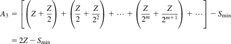
It follows that
Y2=WmaxN2−2(βWmax−N1Smax)+Smin (22)
Because the total number of packets transmitted during a period is also given by 1/p, it follows that
1p=Y1+Y2 (23)
Equation 23 can be used to express Wmax as a function of p. Unfortunately, a closed-form expression for Wmax does not exist in general, but it can computed for the following special cases:
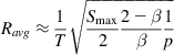
1. βWmax≫2Smax![]()
This condition implies that the window function is dominated by the linear increase part, so that N1>>N2 and from equations 17, 21, and 23, it can be shown that the average throughput is given by
Ravg≈1T√Smax22−ββ1p (24)
 (24)
(24)
which is same as the throughput for a general AIMD congestion control algorithm that was derived in Chapter 2.
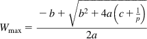
2. βWmax>2Smax![]() and βWmax
and βWmax![]() is divisible by Smax.
is divisible by Smax.
From equations 21 to 23, it follows that
Wmax=−b+√b2+4a(c+1p)2a (25)
 (25)
(25)
where
a=β(2−β)2Smaxb=logSmaxSmin+2−ββc=Smax−Smin
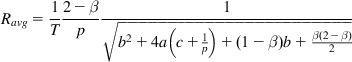
and the throughput is given by
Ravg=1T2−βp1√b2+4a(c+1p)+(1−β)b+β(2−β)2 (26)
 (26)
(26)
3. βWmax≤2Smax![]()
This condition implies that N1=0, and assuming 1p≫Smin![]() , Wmax is approximately given by
, Wmax is approximately given by
Wmax≈1p1log(βWmaxSmin)+2(1−β) (27)
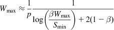 (27)
(27)
This equation can be solved for Wmax in terms of the LambertW(y) function (which is the only real solution to xex=y![]() ) to get
) to get
Wmax=1pln2LambertW(4βe−2βln2ln2pSmin) (28)
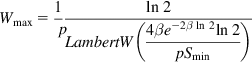 (28)
(28)
so that
Ravg≈Y2TN2=WmaxN2−2βWmaxTN2=WmaxT[1−2βlog(βWmaxSmin)+2] (29)
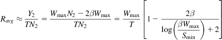 (29)
(29)
From these equations, we can draw the following conclusions:
• Because large values of Wmax also correspond to large link capacities (because Wmax=CT), it follows by a comparison of equations 24 and equation 72 in Chapter 2 that for high-capacity links, BIC operates similar to an AIMD protocol with increase parameter a=Smax, decrease parameter of b=β![]() , and the exponent d=0.5. This follows from the fact that for high-capacity links, the BIC window spends most of its time in the linear increase portion.
, and the exponent d=0.5. This follows from the fact that for high-capacity links, the BIC window spends most of its time in the linear increase portion.
• For moderate values of C, we can get some insight into BIC’s behavior by computing the constants in part 2. As recommended by Xu et al. [1], we choose the following values for BIC’s parameters: β=0.125,Smax=32,Smin=0.01![]() . It follows that a=0.0036, b=18.5, and c=31. 99, and from equation 26, it follows that
. It follows that a=0.0036, b=18.5, and c=31. 99, and from equation 26, it follows that
Ravg=1.875T√1359.02p2+0.014p
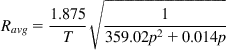
This formula implies that if 359p2>>0.014p, i.e., p>>3.9E(-5), then it follows that
Ravg=0.1Tp
Hence, it follows that for larger packet drop rates (i.e., smaller values of C), the exponent d=1.
Because d=0.5 for large link capacities and d=1 for smaller link capacities, it follows that for intermediate value of capacity 0.5<d<1, which explains the concave shape of the BIC response function Figure 5.4.
Figure 5.7 from Xu et al. [1] shows the variation of the BIC response function as a function of Smax and Smin. Figure 5.7A shows that for a fixed value of Smin, increasing Smax leads to an increase in throughput for large link capacities. Figure 5.7B shows that for a fixed value of Smax, as Smin increases the throughput decreases for lower link capacities.
5.4.2 TCP CUBIC
TCP CUBIC is a follow-on design from the same research group that had earlier come up with TCP BIC [11]. Their main motivation in coming up with CUBIC was to improve on BIC in the following areas: (1) BIC’s window increase function is too aggressive for Reno, especially under short RTT or low-speed networks, and (2) reduce the complexity of BIC’s window increment–decrement rules to make the algorithm more analytically tractable and easier to implement.
Recall that BIC implemented the concave and convex functions that govern the window increase by using a binary search technique. To reduce the resulting complexity of the algorithm, CUBIC replaced the binary search by a cubic function, which contains both concave and convex portions. Another significant innovation in CUBIC is that the window growth depends only on the real time between consecutive congestion events, unlike TCP BIC or Reno in which the growth depends at the rate at which ACKs are returning back to the source. This makes the window growth independent of the round trip latency, so that if multiple TCP CUBIC flows are competing for bandwidth, then their windows are approximately equal. This results in a big improvement in the RTT fairness for CUBIC as shown later in this section.
W(t): Window size at time t, given that the last packet loss occurred at t=0
Wm: Window size at which the last packet loss occurred
α,K![]() : Parameters of the window increase function
: Parameters of the window increase function
β![]() : Multiplicative factor by which the window size is decreased after a packet loss, so that the new window is given by (1−β)Wm
: Multiplicative factor by which the window size is decreased after a packet loss, so that the new window is given by (1−β)Wm![]()
The window size increase function for TCP CUBIC is given by
W(t)=α(t−K)3+Wm (30)
Note that at t=0+, the window size is given by W(0+)=(1−β)Wm![]() , so that
, so that
(1−β)Wm=α(−K)3+Wm,i.e.,
K=3√βWmα (31)
CUBIC runs in one of the following three different modes depending on the value of W(t):
1. CUBIC is in the TCP Mode if W(t) is less than the window size that TCP Reno would reach at time t.
In short RTT networks, TCP Reno can grow faster than CUBIC because its window increases by one every RTT, but CUBIC’s window increase rate is independent of the RTT. To keep CUBIC’s growth rate the same as that of Reno in the situation, CUBIC emulates Reno’s window adjustment algorithm after a packet loss event using an equivalent AIMD (α,β)![]() algorithm as follows: Recall that the throughput for TCP Reno is given by
algorithm as follows: Recall that the throughput for TCP Reno is given by
R=1T√32p

and that for an AIMD (α,β)![]() algorithm is given by
algorithm is given by
R=1T√α(2−β)2β1p
α=3β2−β
will ensure that the AIMD algorithm has the same average throughput as TCP Reno. Because the window size increases by α![]() in every round trip and there are t/T round trips in time t, it follows that the emulated CUBIC window size after t seconds is given by
in every round trip and there are t/T round trips in time t, it follows that the emulated CUBIC window size after t seconds is given by
WAIMD(t)=(1−β)Wm+3β(2−β)tT
If WAIMD is larger than WCUBIC from equation 30, then WCUBIC is set equal to WAIMD. Otherwise, WCUBIC is used as the current congestion window size.
2. If W(t) is greater than the corresponding TCP Reno window but less than Wm, then CUBIC is in the concave region.
3. If W(t) is larger than Wm, then CUBIC is in the convex region.
We now proceed to do an analysis of the throughput for TCP CUBIC. Again using the deterministic approximation technique from Section 2.3, we consider a typical cycle of window increase (Figure 5.9) that is terminated when a packet is dropped at the end of the cycle.
During the course of this cycle, the TCP window increases from (1−β)Wm![]() to Wm
to Wm![]() , and we will assume that this takes on the average τ
, and we will assume that this takes on the average τ![]() seconds. From equation 15, it follows that
seconds. From equation 15, it follows that
τ=3√βWmα (32)
Note that the throughput R(t) at time t, is given by
R(t)=W(t)T (33)
Again, using the deterministic assumption from Section 2.3 of Chapter 2, it follows that the average throughput is given by
Ravg=NτwhereN=1p (34)
is the number of packets transmitted during a cycle. N is also given by
N=τ∫0W(t)Tdt (35)
 (35)
(35)
Following the usual recipe, we equate N to 1/p, where p is the packet drop rate. Hence,
1p=τ∫0W(t)Tdt (36)
 (36)
(36)
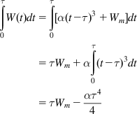
Note that
τ∫0W(t)dt=τ∫0[α(t−τ)3+Wm]dt=τWm+ατ∫0(t−τ)3dt=τWm−ατ44 (37)
 (37)
(37)
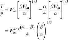
Substituting equations 32 and 37 into equation 35, it follows that
Tp=Wm[βWmα]1/3−α4[βWmα]4/3=W4/3m(4−β)4(βα)1/3 (38)
 (38)
(38)
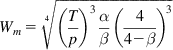
This implies that
Wm=4√(Tp)3αβ(44−β)3 (39)
 (39)
(39)
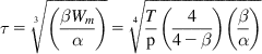
and
τ=3√(βWmα)=4√Tp(44−β)(βα) (40)
 (40)
(40)
The average throughput is then given by
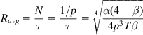
Ravg=Nτ=1/pτ=4√α(4−β)4p3Tβ (41)
 (41)
(41)
From this equation, it follows that the response function for CUBIC is given by
logw=logRavgT=0.25logα(4−β)4β+0.75logT−0.75logp
Because CUBIC is forced to follow TCP Reno for smaller window sizes, its response function becomes
logw={0.25logα(4−β)4β+0.75logT−0.75logpifp<ˉp0.09−0.5logpifp≥ˉp
where
logˉp=logα(4−β)4β+3logT−0.36.
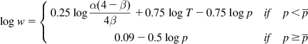
Figure 5.10 clearly shows this piecewise linearity of the CUBIC response function for T=10 ms and T=100 ms, respectively.
Based on these equations, the response function for CUBIC can be regarded as a family of response functions parameterized by the round trip latency T. As shown in Figure 10A, for smaller values of T, the response functions of CUBIC and Reno mostly coincide, but for large values of T (see Figure 5.10B), the CUBIC response function grows faster and looks more like that of HSTCP. This is an interesting contrast with the behavior of HSTCP, in which the switch between HSTCP and TCP Reno happens as a function of the window size W alone, irrespective of the round trip latency T.
The dependency of the Reno–CUBIC cross-over point on T is a very attractive feature because most traffic, especially in enterprise environments, passes over networks with low latency, for whom regular TCP Reno works fine. If a high-speed algorithm is used over these networks, we would like it to coexist with Reno without overwhelming it, and CUBIC satisfies this requirement very well. Over high-speed long-distance networks with a large latency, on the other hand, TCP Reno is not able to make full use of the available bandwidth, but CUBIC naturally scales up its performance to do so.
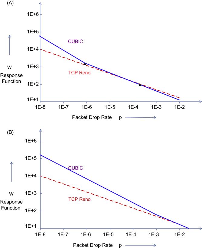
Figure 5.11 shows the ratio between the throughputs of two flows of CUBIC, BIC, HSTCP, and TCP SACK, for a bottleneck link capacity of 400 mbps, and with one of the flows with a fixed RTT of 162 ms; the RTT of the other flow is varied between 16 ms and 162 ms. This clearly shows that CUBIC has better inter-RTT fairness than the other protocols. This can also be inferred from equation 4 because if we substitute e=0.25 and d=0.75, it follows that
R1R2=(T2T1)0.251−0.75=(T2T1).
Hence, TCP CUBIC has better intraprotocol fairness that any of the other high-speed protocols and even TCP Reno. This is because it does not use ACK clocking to time its packet transmissions.
5.5 The Compound TCP (CTCP) Protocol
CTCP was invented by Tan et al. [5,12] from Microsoft Research and serves as the default congestion control algorithm in all operating systems from that company, from Windows Vista onward. In addition to making efficient use of high-speed links, the main design objective of CTCP was to be more TCP friendly compared with the existing alternatives such as HSTCP and CUBIC.
To do so, they came up with an innovative way to combine the fairness of delay-based congestion control approach (as in TCP Vegas) and the aggressiveness of loss-based approaches. Tan et al. [5,12] made the observation that the reason protocols such HSTCP and BIC are not very TCP friendly is that they continue to use the loss-based approach to congestion detection and as a result overload the network. To correct this problem, they suggested that the system should keep track of congestion using the TCP Vegas queue size estimator and use an aggressive window increase rule only when the estimated queue size is less than some threshold. When the estimated queue size exceeds the threshold, then CTCP switches to a less aggressive window increment rule, which approaches the one used by TCP Reno.
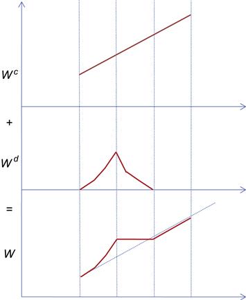
To implement their approach, they used the following decomposition for the window size into two components:
W(t)=Wc(t)+Wd(t) (42)
In equation 42, Wc(t) is the part of the window that reacts to loss-based congestion signals and changes its size according to the rules used by TCP Reno. The component Wd(t), on the other hand, reacts to a delay-based congestion signal and a uses a new set of rules for changing its window size. Specifically, Wd(t) has a rapid window increase rule when the network is sensed to be underutilized and gracefully reduces its size when the bottleneck queue builds up.
W(t): CTCP Window size at time t
Wc(t): Congestion component of the CTCP window size at time t
Wd(t): Delay component of the CTCP window size at time t
T: Base value of the round trip latency
Ts(t): Smoothed estimate of the round trip latency at time t
RE(t): Expected estimate of the CTCP throughput at time t
R(t): Observed CTCP throughput at time t
θ(t)![]() : Delay-based congestion indicator at time t
: Delay-based congestion indicator at time t
γ![]() : Delay threshold, such that the system is considered to b congested if θ(t)≥γ
: Delay threshold, such that the system is considered to b congested if θ(t)≥γ![]()
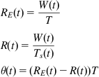
We briefly recap the calculation of the delay-based congestion indicator from TCP Vegas (see Chapter 1):
RE(t)=W(t)TR(t)=W(t)Ts(t)θ(t)=(RE(t)−R(t))T (43)
 (43)
(43)
Note that the expression for θ![]() can also be written as
can also be written as
θ(t)=W(t)Ts(t)(Ts(t)−T) (44)
which by Little’s law equals the number of queued packets in the network.
CTCP specifies that the congestion window should evolve according to the following equations on a per RTT basis:
W←W+αWk,whentherearenopacketlossesorqueuingdelaysand (45)
W←(1−β)WononeormorepacketlossesduringaRTT (46)
Given that the standard TCP congestion window evolves according to (per RTT):
Wc←Wc+1withnoloss,and (47a)
Wc←Wc2withloss (47b)
it follows that the delay-based congestion window Wd![]() should follow the following rules (per RTT):
should follow the following rules (per RTT):
Wd←Wd+[αWk−1]+ifθ≤γ (48a)
Wd←[Wd−ςθ]+ifθ≥γ (48b)
Wd←[(1−β)Wd−Wc2]+withloss (48c)
Using the fact that W=Wc+Wd, it follows from equations 47a and 47b and 48a to 48c that the CTCP window evolution rules (equations 45 and 46) can be written as
W←W+δifW+δ<γ (49a)
W←W0ifW+δ≥W0andWc<W0 (49b)
W←W+1ifWc≥W0 (49c)
W←(1−β)Wwithloss (49c)
where δ=max{⌊αWk⌋,1}![]() and W0 is given by equation 51.
and W0 is given by equation 51.
The shape of the window increase function in equations 49a to 49c (Figures 5.12 and 5.13) is explained as follows: When the network queuing backlog is smaller than γ![]() , the delay-based congestion window grows rapidly as per equation 48a. When the congestion level reaches γ
, the delay-based congestion window grows rapidly as per equation 48a. When the congestion level reaches γ![]() , the congestion window continues to increase at the rate of one packet per round trip time, and the delay window starts to ramp down as per equation 48b. If the rate of increase of the congestion window Wc equals the rate of decrease of the delay window Wd, then the resulting CTCP window W stays constant at W0 until the size of the congestion window Wc exceeds W0. At that point, the CTCP window W resumes its increase at the same linear rate as the congestion window, and the delay window dwindles to zero (see equation 49c).
, the congestion window continues to increase at the rate of one packet per round trip time, and the delay window starts to ramp down as per equation 48b. If the rate of increase of the congestion window Wc equals the rate of decrease of the delay window Wd, then the resulting CTCP window W stays constant at W0 until the size of the congestion window Wc exceeds W0. At that point, the CTCP window W resumes its increase at the same linear rate as the congestion window, and the delay window dwindles to zero (see equation 49c).
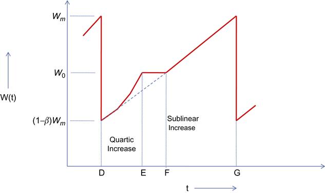
Referring to Figure 5.12, we now derive an expression for the throughput of CTCP using the deterministic sample path–based technique from Section 2.3. The evolution of the window increase is divided into three periods, as explained. Let the duration of these periods be TDE, TEF, and TFG and let NDE, NEF and NFG be the number of packets transmitted over these intervals. Then the average throughput Ravg is given by
Ravg=NDE+NEF+NFGTDE+TEF+TFG (50)
Assuming that the CTCP window size at the end of the cycle is given by Wm, so that the window size at the start of the next cycle is given by (1−β)Wm![]() , we now proceed to compute the quantities in equation 50. Noting that the queue backlog during the interval TEF is given by γ
, we now proceed to compute the quantities in equation 50. Noting that the queue backlog during the interval TEF is given by γ![]() , it follows from Little’s law that
, it follows from Little’s law that
γ=(Ts−T)W0Ts
where W0 is the CTCP window size during this interval. Hence, it follows that
W0=γTsTs−T (51)
During the interval TDE, the CTCP window increases according to
dWdt=αWkTs,sothat (52)
W1−k1−k=αtTs (53)
For the case k=0.75, which is the recommended choice for k as we shall see later, it follows from equation 53 that
W(t)=(αt4Ts)4,tD≤t≤tE
which illustrates the rapid increase in the window size in this region. Because W increases as a power of 4, we refer to this as quartic increase.
Because the window size increases from (1−β)Wm![]() to W0 during the interval TDE, from equation 53, it follows that
to W0 during the interval TDE, from equation 53, it follows that
TDE=Tsα(1−k)[W1−k0−(1−β)1−kW1−km] (54)
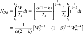
and the number of packets transmitted during this interval is given by (with TDE=tD−tE)
NDE=tE∫tdWTsdt=[α(1−k)Ts]11−k1TstE∫tdt11−kdt=1α(2−k)[W2−k0−(1−β)2−kW2−km] (55)
 (55)
(55)
Note that the interval TEF comes to an end when the size of the congestion window Wc becomes equal to W0. Because dWcdt=1Ts![]() , by equation 47, it follows that
, by equation 47, it follows that
TDF=[W0−(1−β)Wm]Tsand (56)
TEF=TDF−TDE=[W0−(1−β)Wm]Ts−Tsα(1−k)[W1−k0−(1−β)1−kW1−km] (57)
andNEF=W0TEF. (58)
During the interval TFG, the CTCP window increases linearly as for TCP Reno, so that
dWdt=1TssothatΔW=ΔtTs.
Hence,
TFG=(Wm−W0)Tsand (59)
NFG=tG∫tFWTsdt=tG∫tFtT2sdt=t2G−t2F2T2s=W2m−W202 (60)
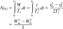 (60)
(60)
Note that the total number of packets transmitted over the interval TDG is also given by 1/p, so that
1p=NDE+NEF+NFG (61)
Equation 61 can be numerically solved to obtain the value of Wm, which can then be substituted back into equations 54, 57, and 59 to obtain the length of the interval TDG. From equation 50, it follows that
Ravg=1/pTDG (62)
If we make the assumption that the packet loss rate is high enough to cause the window size to decrease during the interval TDE, it is possible to obtain a closed-form expression for R. In this case, NDE=1/p so that
1α(2−k)[W2−km−(1−β)2−kW2−km]=1psothat
Wm=[α(2−k)1−(1−β)2−k]12−k1p12−kand (63)
TDE=TsW1−kmα(1−k)[1−(1−β)1−k] (64)
The average throughput Ravg is then given by
Ravg=1pα(1−k)TsW1−km(1−(1−β)1−k)=(αp)12−k1Ts(1−(1−β)1−k)[1−(1−β)2−k2−k]1−k2−k (65)
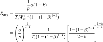 (65)
(65)
To make the variation of the throughput with p the same as that for HSTCP, Tan et al. [5,12] chose k so that 1/(2−k)=0.833, so k=0.8. To make the implementation easier, they used k=0.75 instead.
We can develop some intuition into CTCP’s performance with the following considerations: With reference to Figure 5.12, note that the demarcation between the quartic increase portion of the CTCP window and the linear increase portion is governed by the window size parameter W0 given by
W0=γTsTs−T.
From this equation, it follows that:
• For networks with large latencies, the end-to-end delay is dominated by the propagation delays; hence, Ts≈T![]() . This leads to a large value of W0.
. This leads to a large value of W0.
• For networks with small latencies, the queuing delays may dominate the propagation delays, so that Ts≫T![]() . This leads to small values of W0.
. This leads to small values of W0.
The interesting fact to note is that W0 is independent of the link capacity, which we now use to obtain some insights into CTCP behavior. Also note that in the absence of random link errors, the maximum window size Wm is approximately equal to the delay bandwidth product CT.
Based on the values of the link speed C and the threshold W0, we can have four different scenarios (Figure 5.14):
• As link speed C increases, for a fixed value of end-to-end latency, then Wm increases, and as a result, the number of packets transmitted in the linear portion of window increases (see, e.g., the change from equations 14a to 14b or 14c to 14d). This can also be seen by the formula for NFG in equation 60. As a result, at higher link speeds, the CTCP throughput converges toward that for TCP Reno.
• As the end-to-end latency increases, then W0 increases as explained above, and the number of packets transmitted in the quartic region of the CTCP window increases (see, e.g., the change from equation 14a to 14c or 14b to 14d). This can also be seen by the formula for NDE in equation 55. As a result, an increase in latency causes the CTCP throughput to increase faster compared with that of Reno. This behavior is reminiscent with that of CUBIC because CUBIC’s throughput also increased with respect to Reno as the end-to-end latency increases. However, the CTCP throughput will converge back to that for Reno as the link speed becomes sufficiently large, while the CUBIC throughput keeps diverging.
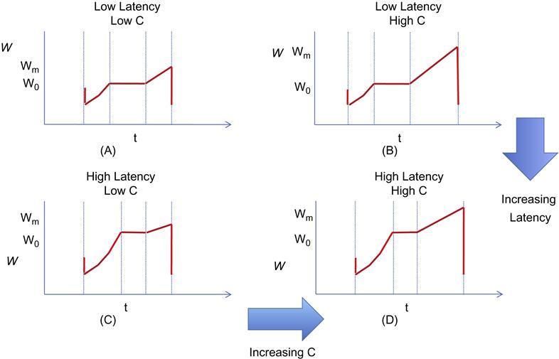
These two effects are clearly evident in the response function plot in Figure 5.15.
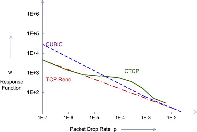
Figure 5.15 plots the response function for CTCP in which the following features are evident: The response functions for Reno and CTCP are close to each other at lower link speeds. Then as the link speed increases, CTCP increases at a faster rate and diverges away from Reno. This can be explained by the fact that the quartic increase portion dominates the linear increase in this region. Finally, when the link speed assumes very large values, to the left part of the graph, CTCP and Reno again converge together. This is because the linear portion of the window increase in CTCP is dominant at high link speeds, as explained earlier.
As the lend-to-end latency increases, we can expect this pattern to persist, with the difference that the portion of the curve where the CTCP response time is bigger will move to the left (because of larger values of W0).
Figure 5.15 also plots the response function for CUBIC for comparison purposes. Observe that response functions for CUBIC starts diverging away from that of Reno as the link speed increases, and unlike CTCP, the divergence keeps increasing. This implies that at very high link speeds CTCP will be at a disadvantage with respect to CUBIC or Reno, as has been noted by Munir et al. [13].
From the discussion in the previous few sections, we observe that there is a fundamental difference between the response function for HSTCP on one hand and that for CUBIC or CTCP on the other. In the latter case, the response function changes as the round trip latency changes and tends to be more TCP Reno friendly at lower latencies. This is an attractive property to have because lower latencies correspond to LAN environments, in which most transfers still use TCP Reno. On the other hand, at higher latencies, both CUBIC and CTCP response functions diverge from that of TCP Reno (CUBIC more so than CTCP). This is tolerable because Reno is not able to make full use of the available link capacity in high-latency and high-capacity networks and may even become unstable.
5.6 The Fast TCP Protocol
The design of FAST TCP was inspired by that of TCP Vegas, and in contrast to the other high-speed protocols, it uses end-to-end delay as a measure of congestion rather than dropped packets. Given the description of TCP Vegas in Chapter 1, the following equation describes the evolution of TCP Vegas’ window size (assuming that the parameters α=β![]() ):
):
Wi(t+1)=Wi(t)+1Ti(t)sgn(αi−Ri(t)θi(t)) (66)
where θi(t)![]() is the queuing delay that connection i experiences, such that the round trip latency is given by Ti(t)=Ti+θi(t)
is the queuing delay that connection i experiences, such that the round trip latency is given by Ti(t)=Ti+θi(t)![]() , where Ti is the fixed part. Hence, Ri(t)θi(t)
, where Ti is the fixed part. Hence, Ri(t)θi(t)![]() is a measure of the number of queued packets from the connection in the network. The function sgn(z)=−1 if z<0, 0 if z=0 and 1 if z>0. Hence, TCP Vegas adjusts its window up or down by one packet per RTT depending on whether the number of queued packets is smaller or greater than its target α
is a measure of the number of queued packets from the connection in the network. The function sgn(z)=−1 if z<0, 0 if z=0 and 1 if z>0. Hence, TCP Vegas adjusts its window up or down by one packet per RTT depending on whether the number of queued packets is smaller or greater than its target α![]() .
.
To create a high-speed version of this algorithm, Wei et al. [7]. changed the window size evolution equation to
Wi(t+1)=Wi(t)+γi(αi−Ri(t)θi(t))γi∈(0,1] (67)
As a result, the window adjustments in FAST TCP depend on the magnitude as well as the sign of the difference αi−Ri(t)θi(t)![]() and are no longer restricted to a change of at most 1 every round trip time. Hence, FAST can adjust its window by a large amount, either up or down, when the number of buffered packets is far away from its target and by a smaller amount when it is closer.
and are no longer restricted to a change of at most 1 every round trip time. Hence, FAST can adjust its window by a large amount, either up or down, when the number of buffered packets is far away from its target and by a smaller amount when it is closer.
It can be shown that FAST has the following property: The equilibrium throughputs of FAST are the unique optimal vector that maximize the sum ∑iαilogRi![]() subject to the link constraint that the aggregate flow rate at any link does not exceed the link capacity. This result was obtained using the Primal-Dual solution to a Lagrangian optimization problem using the methodology described in Chapter 3. Furthermore, the equilibrium throughputs are given by
subject to the link constraint that the aggregate flow rate at any link does not exceed the link capacity. This result was obtained using the Primal-Dual solution to a Lagrangian optimization problem using the methodology described in Chapter 3. Furthermore, the equilibrium throughputs are given by
Ravgi=αi¯θi (68)
Just as for TCP Vegas, equation 68 shows that FAST does not penalize flows with large round trip latencies, although in practice, it has been observed that flows with longer RTTs obtain smaller throughput than those with shorter RTTs. Equation 68 also implies that in equilibrium, source i maintains αi![]() packets in the buffers along its path. Hence, the total amount of buffering in the network is at least ∑iαi
packets in the buffers along its path. Hence, the total amount of buffering in the network is at least ∑iαi![]() to reach equilibrium. Wang et al. [14] have also proven a stability result for FAST, which states that it is locally asymptotically stable in general networks when all the sources have a common round trip delay, no matter how large the delay is.
to reach equilibrium. Wang et al. [14] have also proven a stability result for FAST, which states that it is locally asymptotically stable in general networks when all the sources have a common round trip delay, no matter how large the delay is.
5.7 The eXpress Control Protocol (XCP)
The XCP congestion control algorithm [15] is an example of a “clean slate” design, that is, it is a result of a fundamental rethink of the congestion control problem without worrying about the issue of backward compatibility. As a result, it cannot deployed in a regular TCP/IP network because it requires multi-bit feedback, but it can be used in a self-contained network that is separated from the rest of the Internet (which can done by using the split TCP architecture from Chapter 4, for example).
XCP fundamentally changes the nature of the feedback from the network nodes by having them provide explicit window increase or decrease numbers back to the sources. It reverses TCP’s design philosophy in the sense that all congestion control intelligence is now in the network nodes. As a result, the connection windows can be adjusted in a precise manner so that the total throughput at a node matches its available capacity, thus eliminating rate oscillations. This allows the senders to decrease their windows rapidly when the bottleneck is highly congested while performing smaller adjustments when the sending rate is close to the capacity (this is similar to the BIC and CUBIC designs and conforms to the averaging principle). To improve system stability, XCP reduces the rate at which it makes window adjustments as the round trip latency increases.
Another innovation in XCP is the decoupling of efficiency control (the ability to get to high link utilization) from fairness control (the problem of how to allocate bandwidth fairly among competing flows). This is because efficiency control should depend only on the aggregate traffic behavior, but any fair allocation depends on the number of connections passing through the node. Hence, an XCP-based AQM controller has both an efficiency controller (EC) and a fairness controller (FC), which can be modified independently of the other. In regular TCP, the two problems coupled together because the AIMD window increase–decrease mechanism is used to accomplish both objectives, as was shown in the description of the Chiu-Jain theory in Chapter 1.
5.7.1 XCP Protocol Description
The XCP protocol works as follows:
• Traffic source k maintains a congestion window Wk, and keeps track of the round trip latency Tk. It communicates these numbers to the network nodes via a congestion header in every packet. Note that the rate Rk at source k is given by
Rk=WkTk
Whenever a new ACK arrives, the following equation is used to update the window:
Wk←Wk+Sk (69)
where Sk is explicit window size adjustment that is computed by the bottleneck node and is conveyed back to the source in the ACK packet. Note that Sk can be either positive or negative, depending on the congestion conditions at the bottleneck.
• Network nodes monitor their input traffic rate. Based on the difference between the link capacity C and the aggregate rate Y given by Y=∑Kk=1Rk![]() , the node tells the connections sharing the link to increase or decrease their congestion windows, which is done once every average round trip latency, for all the connections passing through the node (this automatically reduces the frequency of updates as the latencies increase). This information is conveyed back to the source by a field in the header. Downstream nodes can reduce this number if they are experiencing greater congestion, so that in the end, the feedback ACK contains information from the bottleneck node along the path.
, the node tells the connections sharing the link to increase or decrease their congestion windows, which is done once every average round trip latency, for all the connections passing through the node (this automatically reduces the frequency of updates as the latencies increase). This information is conveyed back to the source by a field in the header. Downstream nodes can reduce this number if they are experiencing greater congestion, so that in the end, the feedback ACK contains information from the bottleneck node along the path.
• Operation of the Efficiency Controller (EC): The EC’s objective is to maximize link utilization while minimizing packet drops and persistent queues. The aggregate feedback ϕ![]() (in bytes) is computed as follows:
(in bytes) is computed as follows:
ϕ=αTav(C−∑Kk=1Rk)−βb (70)
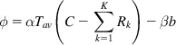 (70)
(70)where α,β![]() are constants whose values are set based on the stability analysis, Tav is the average round trip latency for all connections passing through the node, and b is the minimum queue seen by an arriving packet during the last round trip interval (i.e., it’s the queue that does not drain at the end of a round trip interval). The first term on the RHS is proportional to the mismatch between the aggregate rate and the link capacity (multiplied by the round trip latency to convert it into bytes). The second term is required for the following reason: When there is a persistent queue even if the rates in the first term are matching, then the second term helps to reduce this queue size.
are constants whose values are set based on the stability analysis, Tav is the average round trip latency for all connections passing through the node, and b is the minimum queue seen by an arriving packet during the last round trip interval (i.e., it’s the queue that does not drain at the end of a round trip interval). The first term on the RHS is proportional to the mismatch between the aggregate rate and the link capacity (multiplied by the round trip latency to convert it into bytes). The second term is required for the following reason: When there is a persistent queue even if the rates in the first term are matching, then the second term helps to reduce this queue size.
From the discussion in Chapter 3, the first term on the RHS in equation 7 is proportional to the derivative of the queue length, and the second term is proportional to the difference between the current queue size and the target size of zero. Hence, the XCP controller is equivalent to the proportional-integral (PI) controller discussed in Chapter 3.
Note that the increase in transmission rates in XCP can be very fast because the increase is directly proportional to the spare link bandwidth as per equation 70, which makes XCP suitable for use in high-speed links. This is in contrast to TCP, in which the increase is by at most one packet per window.
• Operation of the Fairness Controller (FC): The job of the FC is to divide up the aggregate feedback among the K connections in a fair manner. It achieves fairness by making use of the AIMD principle, so that:
– If ϕ![]() >0, then the allocation is done so that the increase in throughput for all the connections is the same.
>0, then the allocation is done so that the increase in throughput for all the connections is the same.
– If ϕ![]() <0, then the allocation is done so that the decrease in throughput of a connection proportional to its current throughput.
<0, then the allocation is done so that the decrease in throughput of a connection proportional to its current throughput.
When ϕ![]() is approximately zero, then the convergence to fairness comes to a halt. To prevent this, XCP does an artificial deallocation and allocation of bandwidth among the K connections by using the feedback h given by
is approximately zero, then the convergence to fairness comes to a halt. To prevent this, XCP does an artificial deallocation and allocation of bandwidth among the K connections by using the feedback h given by
h=max(0,0.1∑Kk=1Rk−|ϕ|), (71)
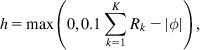 (71)
(71)so on every RTT, at least 10% of the traffic is redistributed according to AIMD. This process is called “bandwidth shuffling” and is the principle fairness mechanism in XCP to redistribute bandwidth among connections when a new connection starts up.
The per packet feedback to source k can be written as
ϕk=pk−nk (72)
where pk is the positive feedback and nk is the negative feedback.
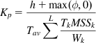
First consider the case when ϕ![]() >0. This quantity needs to be equally divided among the throughputs of the K connections. The corresponding change in window size of the kth connection is given by ΔWk=ΔRkTk∝Tk
>0. This quantity needs to be equally divided among the throughputs of the K connections. The corresponding change in window size of the kth connection is given by ΔWk=ΔRkTk∝Tk![]() because the throughput deltas are equal. This change needs to be split equally among the packets from connection k that pass through the node during time Tk, say mk. Note that mk is proportional to Wk/MSSk
because the throughput deltas are equal. This change needs to be split equally among the packets from connection k that pass through the node during time Tk, say mk. Note that mk is proportional to Wk/MSSk![]() and inversely proportional to Tk. It follows that the change in window size per packet for connection k is given by
and inversely proportional to Tk. It follows that the change in window size per packet for connection k is given by
pk=KpT2kMSSkWk (73)
where Kp is a constant. Because the total increase in aggregate traffic rate is h+max(ϕ,0)Tav![]() , it follows that
, it follows that
h+max(ϕ,0)Tav=∑LpkTk (74)
where the summation is over the average number of packets seen by the node during an average RTT. Substituting equation 73 into equation 74, we obtain
Kp=h+max(ϕ,0)Tav∑LTkMSSkWk (75)
 (75)
(75)
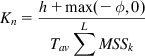
When ϕ![]() <0, then the decrease in throughput should be proportional to the current throughput. It follows that ΔWk=ΔRkTk∝RkTk=Wk
<0, then the decrease in throughput should be proportional to the current throughput. It follows that ΔWk=ΔRkTk∝RkTk=Wk![]() . Splitting up this change in window size among all the mk packets that pass through the node during an RTT, it follows that
. Splitting up this change in window size among all the mk packets that pass through the node during an RTT, it follows that
nk=KnWkmk=KnTkMSSk (76)
where the constant Kn is given by
Kn=h+max(−ϕ,0)Tav∑LMSSk (77)
 (77)
(77)
5.7.2 XCP Stability Analysis
In this section, we show that the if parameters α,β![]() (that appear in equation 70) satisfy the conditions:
(that appear in equation 70) satisfy the conditions:
0<α<π4√2andβ=α2√2 (78)
then the system is stable, independently of delay, capacity, and number of connections. This analysis is done using the techniques introduced in Chapter 3, whereby the system dynamics with feedback are captured in the fluid limit using ordinary differential equations, to which the Nyquist stability criterion is applied.
In this section, we will assume that the round trip latencies for all the k connections are equal, so that Tk=Tav=T, k=1,…,K. Using the notation used in the previous section, note that the total traffic input rate into the bottleneck queue is given by
Y(t)=∑Kk=1Rk(t)=∑Kk=1Wk(t)T (79)
Because the aggregate feedback ϕ![]() is divided up among the K connections, every T seconds, it follows that the total rate of change in their window sizes is given by ϕ/T
is divided up among the K connections, every T seconds, it follows that the total rate of change in their window sizes is given by ϕ/T![]() bytes/sec. Using equation 70, it follows that
bytes/sec. Using equation 70, it follows that
∑Kk=1dWkdt=1T[−αT(y(t−T)−C)−βb(t−T)] (80)
From equations 79 and 80, it follows that
dY(t)dt=1T2[−αT(Y(t−T)−C)−βb(t−T)] (81)
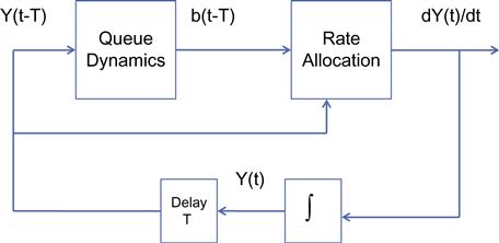
Hence, the equations that govern the input traffic rate and buffer dynamics are the following
db(t)dt={Y(t)−Cifb(t)>0max(0,Y(t)−C)ifb(t)=0 (82)
dYdt=−αT(Y(t−T)−C)−βT2b(t−T) (83)
These form a feedback loop, as shown in Figure 5.16. In this figure, the queue dynamics are governed by equation 82, and the rate allocation is done via equation 83. These equations have the equilibrium point beq=0 and Yeq=C. If we consider the following linear equations around this equilibrium point, by making the substitution x(t)=Y(t)−C, we get
db(t)dt=x(t) (84)
dx(t)dt=−K1x(t−T)−K2b(t−T) (85)
where
K1=αTandK2=βT2 (86)
Passing to the Laplace transform space, it follows from equations 84 and 85 that the open loop transfer function for the system is given by
G(s)=sK1+K2s2e−sT (87)
To apply the Nyquist Criterion, we express equation 87 in the complex plane by making the substitution s=jω![]() , so that
, so that
G(jω)=|G(jω)|e−arg(G(jω))
where
|G(jω)|=√ω2K21+K22ω2 (88)
and
arg(G(jω))=π−tan−1ωK1K2+ωT (89)
We now choose the critical frequency ωc![]() at which |G(jωc)|=1
at which |G(jωc)|=1![]() , as a function of the parameters K1 and K2 as follows
, as a function of the parameters K1 and K2 as follows
ωc=K2K1 (90)
Using equation 88, it follows that K2K21=√2![]() , which can be expressed using equation 86 as β=α2√2
, which can be expressed using equation 86 as β=α2√2![]() .
.
To prove stability of the closed-loop system, the Nyquist criterion requires that arg(G(jωc))<π![]() radians. Substituting equation 90 into equation 89, it follows that
radians. Substituting equation 90 into equation 89, it follows that
arg(G(jωc))=π−π4+βα<πi.e.α<π4√2
which completes the proof.
This analysis shows that unlike for traditional congestion control and AQM schemes, XCP’s stability criterion is independent of the link capacity, round trip latency, or number of connections. It was later shown by Balakrishnan et al. [16] that the linearization assumption around the point beq=0 may not be a good approximation because the system dynamics are clearly nonlinear at this point (see equation 82). They did a more exact stability analysis using Lyapunov functionals and showed that the more exact stability region for α,β![]() varies as a function of T and is in fact much larger than the region given by equation 78. However, it is not an exact superset because there are points near the boundary of the curve β=α2√2
varies as a function of T and is in fact much larger than the region given by equation 78. However, it is not an exact superset because there are points near the boundary of the curve β=α2√2![]() that lie in the stable region as per the linear analysis but actually lie in the unstable region according to the nonlinear analysis (see Balakrishnan et al. [16]).
that lie in the stable region as per the linear analysis but actually lie in the unstable region according to the nonlinear analysis (see Balakrishnan et al. [16]).
5.8 The Rate Control Protocol (RCP)
The RCP protocol [17] was inspired by XCP and builds on it to assign traffic rates to connections in a way such that they can quickly get to the ideal Processor Sharing (PS) rate. RCP is an entirely rate-based protocol (i.e., no windows are used). Network nodes compute the ideal PS-based rate and then pass this information back to the source, which immediately changes its rate to the minimum PS rate that was computed by the nodes that lie along its path.
RCP was designed to overcome the following issue with XCP: When a new connection is initiated in XCP and the nodes along its path are already at their maximum link utilizations, then XCP does a gradual redistribution of the link capacity using the bandwidth-shuffling process (see equation 71). Dukkipatti and McKeown [17] have shown that this process can be quite slow because new connections start with a small window and get to a fair allocation of bandwidth in a gradual manner by using the AIMD principle. However, it takes several round trips before convergence happens, and for smaller file sizes, the connection may never get to a fair bandwidth distribution. Hence, one of the main innovations in RCP, compared with XCP, is that the bandwidth reallocation happens in one round trip time, in which a connection gets its equilibrium rate.
The RCP algorithm operates as follows:
• Every network node periodically computes a fair-share rate R(t) that it communicates to all the connections that pass through it. This computation is done approximately once per round trip delay.
• RCP mandates two extra fields in the packet header: Each network node fills field 1 with is fair share value R(t), and when the packet gets to the destination, it copies this field into the ACK packet sends it back to the source. Field 2, as in XCP, is used communicate the current average round trip latency Tk, from a connection to all the network nodes on its path. The nodes use this information to compute the average round trip latency Tav of all the connections that pass through it.
• Each source transmits at rate Rk, which is the smallest offered rate along its path.
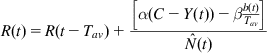
• Each network node updates its local rate R(t) according to the equation below:
R(t)=R(t−Tav)+[α(C−Y(t))−βb(t)Tav]ˆN(t) (91)
 (91)
(91)
where ˆN(t)![]() is the node’s estimate of the number of connections that pass through it and the other variables are as defined for XCP.
is the node’s estimate of the number of connections that pass through it and the other variables are as defined for XCP.
The basic idea behind equation 91 is that if there is spare bandwidth available (equal to C−Y(t)), then share it equally among all the connections; on the other hand, if C−Y(t)<0, then the link is over subscribed, and each connection is asked to decrease its rate evenly. If there is a queue build-up of b(t), then a rate decrease of b(t)/Tav will bring it down to zero within a round trip interval.
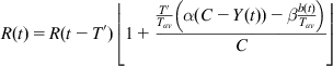
RCP replaces the interval at which the node recomputes R(t) to T′, so that it is user configurable and uses the following estimate for the number of connections:
ˆN(t)=CR(t−T′)
so that equation 91 can be written as
R(t)=R(t−T′)⌊1+T′Tav(α(C−Y(t))−βb(t)Tav)C⌋ (92)
 (92)
(92)
where the rate change has been scaled down by T′/Tav because it is done more than once per Tav seconds.
It can be easily shown that system dynamic equations for RCP are exactly the same as for XCP (see equations 82 and 83). Hence, the stability conditions derived for XCP in the previous section hold in this case as well.
5.9 Stability of High-Speed TCP Algorithms
The algorithms described in this chapter all operate in the region where regular TCP has been shown to exhibit poor performance because of oscillatory behavior. From the analysis that was described in Chapter 3, the following techniques were found to increase the stability of congestion control algorithms in networks with high link capacity or end-to-end latency:
• Sophisticated AQM schemes that feed back the buffer occupancy value, as well as the first or higher derivatives of the buffer occupancy. Note that the first derivative of the buffer occupancy is given by
db(t)dt=C−∑iRi
so that it provides the same information as the difference between the link capacity and the current traffic load (i.e., how close the link is to saturation).
• Window size increment rules that incorporate the Averaging Principle (AP) to reduce the rate of the window size increase as the link approaches saturation
The natural question to ask is how do the algorithms described in this chapter fare in this regard? We have not seen any work that applies control theory to models for HSTCP, BIC, CUBIC, or CTCP, but simulations show that they are much more stable than Reno in the high-link speed and large propagation delay environment.
A reason why this is the case can be gleaned from the principles enunciated earlier. Applying the Averaging Principle, algorithms that reduce the window increment size as the link reaches saturation, are more stable than those that do not do so. BIC, CUBIC, CTCP, and FAST all fall into this category of algorithms. BIC, CUBIC, and FAST reduce their window increment size in proportion to how far they are from the link saturation point while CTCP changes to a linear rate of increase (from quartic) when the queue backlog increases beyond a threshold. XCP and RCP, on the other hand, use a sophisticated AQM scheme in which the network nodes feed back the value of the buffer occupancy as well as the difference between the link capacity and the total traffic load. The Quantum Congestion Notification (QCN) algorithm that we will meet in Chapter 8 uses a combination of the averaging principle and first derivative feedback to achieve stability.
The HSTCP algorithm, on the other hand, does not fall cleanly into one of these categories. But note that HSTCP decreases its window size decrement value (on detecting packet loss) as the window size increases, and in general, algorithms that do a less drastic reduction of their window size compared with Reno have better stability properties (because this has the effect of reducing the rate oscillations). This is also true for TCP Westwood (see Chapter 4), whose window size reduction is proportional to the amount of queuing delay. The Data Center Congestion Control Protocol (DCTCP) algorithm (see Chapter 7) also falls in this class because it reduces its window size in proportion to the amount of time that the queue size exceeds some threshold.
5.10 Further Reading
Other TCP algorithms designed for high-speed long latency links include Scalable TCP [18], H-TCP [19], Yeah-TCP [6], TCP Africa [9], and TCP Illinois [4]. All of these are deployed on fewer than 2% of the servers on the Internet, according to the study done by Yang et al. [8].