Congestion Control in Data Center Networks
This chapter explores congestion control in data center networks (DCNs). This is the most current and still rapidly evolving area because of the enormous importance of DCNs in running the data centers that underlie the modern Internet economy. Because DCNs can form a relatively autonomous region, there is also the possibility of doing a significant departure from the norm of congestion control algorithms if the resulting performance is worth it. This has resulted in innovations in congestion control such as the application of ideas from Earliest Deadline First scheduling and even in-network congestion control techniques. All of these are driven by the need to keep the end-to-end latency between two servers in a DCN to values that are in the tens of milliseconds or smaller to satisfy the real-time needs to applications such as Web search and social networking.
Keywords
congestion control in Data Center Networks; DCN; tree-based DCN; bisection bandwidth; VL2 Inter-Connection Network; Fat Tree Inter-Connection Network; data center TCP; DCTCP; HULL and DCTCP; Deadline Aware Data Center TCP; D2TCP; D3 Congestion Control Algorithm; Preemptive Distributed Quick Flow algorithm; PDQ; Multipath TCP; Incast Problem; pFabric congestion control algorithm; Detail congestion control algorithm
7.1 Introduction
This chapter discusses the topic of congestion control in data center networks (DCN), which have assumed a lot of importance in the networking arena lately. DCNs are used to create “cloud”-based massively parallel information processing systems, which are integral to the way computing is done today. They underlie the massive computing infrastructure that run web sites such as Google and Facebook and constitute a key competitive advantage for these types of companies.
Modern data centers are created by interconnecting together a large number of commodity servers and their associated storage systems, with commodity Ethernet switches. They create a “warehouse-scale” computing infrastructure [1] that scales “horizontally”; that is, we can increase the processing power of the data center by adding more servers as opposed to increasing the processing power of individual servers (which is a more expensive proposition). The job of a DCN in the data center architecture is to interconnect the servers in a way that maximizes the bandwidth between any two servers while minimizing the latency between them. The DCN architecture should also allow the flexibility to easily group together servers that are working on the same application, irrespective of where they are located in the DCN topology.
From the congestion control point of view, DCNs have some unique characteristics compared with the other types of Internet Protocol (IP) networks that we have seen so far in this book:
• The round trip latencies in DCNs are extremely small, usually of the order of a few hundred microseconds, as opposed to tens of milliseconds and larger for other types of networks.
• Applications need very high bandwidths and very low latencies at the same time.
• There is very little statistical multiplexing, with a single flow often dominating a path.
• To keep their costs low, DCN switches have smaller buffers compared with regular switches or routers because vendors implement them using fast (and expensive) static random-access memory (SRAM) to keep up with the high link speeds. Moreover, buffers are shared between ports, so that a single connection can end up consuming the buffers for an entire switch [2].
As a result of these characteristics, normal TCP congestion control (i.e., TCP Reno) does not perform very well because of the following reasons:
• TCP requires large buffers; indeed, the buffer size should be greater than or equal to the delay-bandwidth product of the connection to fully use the full bandwidth of the link as shown in Chapter 2.
• End-to-end delays of connections under TCP are much larger than what can be tolerated in DCNs. The delays are caused by TCP’s tendency to fill up link buffers to capacity to fully use the link.
Another special characteristic of DCNs is that they are homogeneous and under a single administrative control. Hence, backward compatibility, incremental deployment, or fairness to legacy protocols are not of major concern. As a result, many of the new DCN congestion control algorithms require fairly major modifications to both the end systems as well as the DCN switches. Their main objective is to minimize end-to-end latency so that it is of the order of a few milliseconds while ensuring high link utilization.
DCN congestion control algorithms fall in two broad categories:
• Algorithms that retain the end-to-end congestion control philosophy of TCP: Data Center TCP (DCTCP) [2], Deadline-Aware Data Center TCP (D2TCP) [3], and High bandwidth Ultra Low Latency (HULL) [4], fall into this category of algorithms. They use a more aggressive form of a Random Early Detection (RED)–like Explicit Congestion Notification (ECN) feedback from congested switches that are then used to modify the congestion window at the transmitter. These new algorithms are necessitated due to the fact that Normal RED or even the more effective form of Active Queue Management (AQM) with the Proportional-Integral (PI) controller (see Chapter 3) is not able to satisfy DCNs’ low latency requirements.
• Algorithms that depend on in-network congestion control mechanisms: Some recently proposed DCN congestion control protocols such as D3 [5], Preemptive Distributed Quick Flow Scheduling (PDQ) [6], DeTail [7], and pFabric [8] fall in this category. They all use additional mechanisms at the switch, such as bandwidth reservations in D3, priority scheduling in pFabric or packet by packet load balancing in DeTail. The general trend is towards a simplified form of rate control in the end systems coupled with greater support for congestion control in the network because this leads to much faster response to congestion situations. This is a major departure from the legacy congestion control philosophy of putting all the intelligence in the end system.
To communicate at full speed between any two servers, the interconnection network provides multiple paths between them, which is one of the distinguishing features of DCNs. This leads to new open problems in the area of how to load balance the traffic among these paths. Multi-path TCP (MPTCP) [9,10] is one of the approaches that has been suggested to solve this problem, using multiple simultaneous TCP connections between servers, whose windows are weakly interacting with one another.
The Incast problem is a special type of traffic overload situation that occurs in data centers. It is caused by the way in which jobs are scheduled in parallel across multiple servers, which causes their responses to be synchronized with one another, thus overwhelming switch buffers.
The rest of this chapter is organized as follows: Section 7.2 provides a brief overview to the topic of DCN Interconnect networks. We also discuss the traffic generation patterns in DCNs and the origin of the low latency requirement. Section 7.3 discusses the DCTCP algorithm, and Section 7.4 explores Deadline Aware algorithms, including D2TCP and D3. Section 7.5 is devoted to MPTCP, and Section 7.6 describes the Incast problem in DCNs.
An initial reading of this chapter can be done in the sequence 7.1→7.2→7.3→7.5, which contains an introduction to data center architectures and a description and analysis of the DCTCP and Multipath TCP algorithms. More advanced readers can venture into Sections 7.4 and 7.6, which discuss deadline aware congestion control algorithms and the Incast problem.
7.2 Data Center Architecture and Traffic Patterns
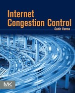
A typical data center consists of thousands of commodity servers that are connected together using a special type of Ethernet network called an Inter-connection Network. An example of a data center using a traditional tree-type interconnection architecture is shown in Figure 7.1, which illustrates the main features of this type of network: Servers are arranged in racks consisting of 20 to 40 devices, each of which is connected to a Top of Rack (ToR) switch. Each ToR is connected to two aggregation switches (ASs) for redundancy, perhaps through an intermediate layer of L2 switches. Each AS is further connected to two aggregation routers (ARs), such that all switches below each pair of ARs form a single Layer 2 domain, connecting several thousand servers. Servers are also partitioned into Virtual Local Area Networks (VLANs) to limit packet flooding and Address Resolution Protocol (ARP) broadcasts and to create a logical server group that can be assigned to a single application. ARs in turn are connected to core routers (CRs) that are responsible for the interconnection of the data center with the outside world.
Some of the problems with this architecture include the following:
• Lack of bisection bandwidth: Bisection bandwidth is defined as the maximum capacity between any two servers. Even though each server may have a 1-Gbps link to its ToR switch and hence to other servers in its rack, the links further up in the hierarchy are heavily oversubscribed. For example, only 4 Gbps may be used on the link between the ToR and AS switches, resulting in 1:5 oversubscription when there are 20 servers per rack, and paths through top-most layers of the tree may be as much as 1:240 oversubscribed. As a result of this, designers tend to only user servers that are closer to each other, thus fragmenting the server pool (i.e., there may be idle servers in part of the data center that cannot be used to relieve the congestion in another portion of the system).
Note that bisection bandwidth is a very important consideration in DCNs because the majority of the traffic is between servers, as opposed to between servers and the external network. The reason for this is that large DCNs are used to execute applications such as Web search, analytics, and so on that involve coordination and communication among subtasks running on hundreds of servers using technologies such as map-reduce.
• Configuration complexity: Another factor that constrains designers to use servers in the same Layer 2 domain for a single service is that adding additional servers to scale the service outside the domain requires reconfiguration of IP addresses and VLAN trunks because IP addresses are topologically significant and are used to route traffic to a particular Layer 2 domain. As a result, most designs use a more static policy whereby they keep additional servers idle within the same domain to scale up, thus resulting in server under-utilization.
• Poor reliability and redundancy: Within a Layer 2 domain, the use of Spanning Tree protocol for data forwarding results in only a single path between two servers. Between Layer 2 domains, up to two paths can be used if Equal Cost Multi-Path (ECMP) [11] routing is turned on.
To address these problems, several new data center architectures have been proposed in recent years. Some of the more significant designs include the following:
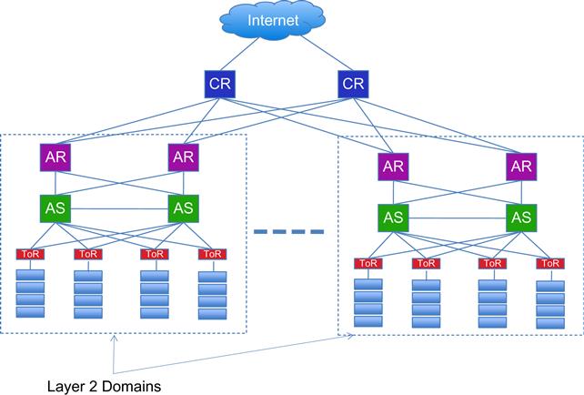
The VL2 Inter-Connection Network: Instead of using the Tree Architecture, Greenberg et al. [12] proposed using a Clos network [13] of interserver connections (Figure 7.2). As shown, each ToR switch is still connected to two AS switches using 1-Gbps links, but unlike the Tree Architecture, each AS switch is connected to every other AS switch in 2-hops, through a layer of intermediate switches (ISs) using 10 Gbps or higher speed links. As a result, if there are n IS switches, then there are n paths between any two ASs, and if any of the IS fails, then it reduces the bandwidth between 2 AS switches by only 1/n. For the VL2 network shown in Figure 7.2, the total capacity between each layer is given by DIDA/2 times the link capacity, assuming that there are DI AS switches with DA ports each. Also note that the number of ToR switches is given by DADI/4, so that if there are M servers attached with a 1-Gbps link to the ToR and the links between the AS and IS are at 10 Gbps, then equating the total bandwidth from the AS to the ToR switches to the total bandwidth in the opposite direction, we obtain
servers per ToR, so that the network can support a total of 5DADI servers, with a full bisection bandwidth of 1 Gbps between any two servers.
The VL2 architecture uses Valiant Load Balancing (VLB) [14] among flows to spread the traffic through multiple paths. VLB is implemented using ECMP forwarding in the routers. VL2 also enables the system to create multiple Virtual Layer 2 switches (hence the name), such that it is possible to configure a virtual switch with servers that may be located anywhere in the DCN. All the servers in Virtual Switch are able to communicate at the full bisection bandwidth and furthermore are isolated from servers in the other Virtual Switches.
To route packets to a target server, the system uses two sets of IP addresses. Each application is assigned an Application Specific IP Address (AA), and all the interfaces in the DCN switches are assigned a Location Specific IP Address (LA) (a link-state based IP routing protocol is used to disseminate topology information among the switches in the DCN). An application’s AA does not change if it migrates from server to server, and each AA is associated with an LA that serves as the identifier of the ToR switch to which it is connected. VL2 has a Directory System (DS) that stores the mapping between the AAs and LAs. When a server sends a packet to its ToR switch, the switch consults the DS to find out the destination ToR and then encapsulates the packet at the IP level, known as tunneling, and forwards it into the DCN. To take advantage of the multiple paths, the system does load balancing at the flow level by randomizing the selection of the Intermediate Switch used for the tunnel. Data center networking–oriented switching protocols such as VxLAN and TRILL use a similar design.
A VL2-based DCN can be implemented using standard switches and routers, the only change required is the addition of a software layer 2.5 shim in the server protocol stack to implement address resolution and tunnel selection functions.
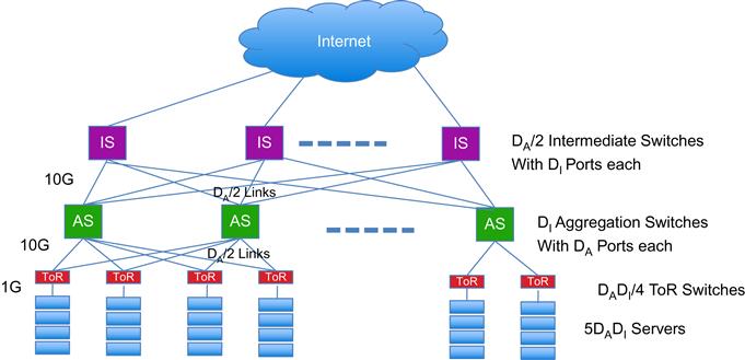
The Fat Tree Architecture: Vahdat et al. [15] proposed another Clos-based DCN architecture called Fat Tree (Figure 7.3). The network is built entirely with k-port 1-Gbps switches and is constructed around k pods, each of which has two layers of switches, with (k/2) switches in each layer. The bottom layer of switches in a pod is connected to the servers, with (k/2) servers connected to each switch. This implies that the system with k pods can connect (k/2) switches/pod * (k/2) server facing ports per switch * k pods=(k3/4) servers per network. Similarly, it can be shown that there are k2/4 core switches per network, so that the number of equal-cost multipaths between any pair of hosts is also given by k2/4. Because the total bandwidth between the core switch and aggregation switch layers is given by k3/4, it follows that the network has enough capacity to support a full 1-Gbps bisectional bandwidth between any two servers in the ideal case.
The main distinction compared with VL2 is the fact that the Fat Tree network is built entirely out of lower speed 1 Gbps switches. However, this come at the cost of larger number of interconnections between switches. To take full advantage of the Fat Tree topology and realize the full bisection bandwidth, the traffic between two servers needs to be spread evenly between the (k/2)2 paths that exist between them. It is not possible to do this using the traditional ECMP-based IP routing scheme, so Vahdat et al. designed a special two-level routing table scheme to accomplish this.
Modern data center designs use a simpler form the Clos architecture called Leaf Spine. VL2 is an example of a 3-Layer Leaf Spine design with ToR, AS and IS switches forming the three layers. It is possible to do a 2-Layer Leaf Spine design with just the ToR and IS layers, with each ToR switch directly connected to every one of the IS switches.
As both the VL2 and the Fat Tree interconnections illustrate, the biggest difference between DCNs and more traditional networks is the existence of multiple paths between any two servers in a DCN. This opens the field to new types of congestion control algorithms that can take advantage of this feature.
7.2.1 Traffic Generation Model and Implications for Congestion Control
We provide a short description of a typical online transaction that generates most of the traffic in large DCNs today (Figure 7.4). Applications such as web search, social network content composition, and advertisement selection are all based around this design pattern. Each of the nodes in Figure 7.4 represents the processing at a server node; the connector between nodes stands for the transmission of a flow across the interconnection network. A typical online transaction is generated when a user enters a query into a search engine. Studies have shown that the response needs to be generated within a short deadline of 230 to 300 ms. A very large data set is required to answer the query, which is spread among thousands of servers in the DCN, each with its own storage. The way a query progresses through a DCN is shown in Figure 7.4. The query arrives at the root node, which broadcasts it to down to the next level, which in turn generate their own queries one level down until the leaf nodes holding the actual data are reached. Each leaf node sends its response back to its parent, which aggregates the replies from all its child nodes and sends it up to the root. Furthermore, answering a query may involve iteratively invoking this pattern; one to four iterations are typical, but as many as 20 may occur.
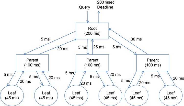
This overall architecture is called scatter-gather, partition-aggregate, or map-reduce. The propagation of the request down to the leaves and the responses back to the root must complete within the overall deadline that is allocated to the query; otherwise, the response is discarded. To satisfy this, the system allocates a deadline to each processing node, which gets divided up into two parts: the computation time in the leaf node and the communication latency between the leaf and the parent. The deadlines for individual computational nodes typically vary from about 10 to 100 ms. Some example delay allocations to the nodes and the communications links are shown in Figure 7.4, from which we can see that the deadlines for communications between hosts cannot exceed tens of milliseconds if the system is to be able to meet the overall job deadline.
This model of data center job computation leads to a few different models for congestion control algorithms that are optimized for DCNs, namely:
• Minimization of flow latency becomes a very important requirement in DCNs, which was not the case for other congestion control scenarios. At the same time, other flows in the data center are throughput intensive. For example, large transfers that update the internal data structures at a server node fall into the latter category; hence, throughput maximization and high link utilization cannot be ignored as the congestion control objective. Based on this insight, a number of new congestion control algorithms, such as DCTCP, try to minimize latency with an aggressive form of AQM while not compromising on throughput.
• A second class of algorithms tackles the issue of deadlines for flows directly by using congestion control algorithms that take these deadlines into account. Algorithms such as D3 [5] and D2TCP [3] fall in this category.
• A third class of algorithms have adopted a more radical design by parting ways with the “all intelligence should be in the end system” philosophy of the Internet. They contend that end system–based controls have an unsurmountable delay of one round trip before they can react to network congestion, which is too slow for DCNs. Instead they propose to make the network responsible for congestion control while limiting the end system to very simple nonadaptive rate regulation and error recovery functions. Some of these algorithms take advantage of the fact that there are multiple paths between any two servers; hence, the network nodes can quickly route around a congested node on a packet-by-packet basis (e.g., see [7]).
7.3 Data Center TCP (DCTCP)
DCTCP was one of the earliest congestion control algorithms designed for DCNs and is also one of the best known. It was invented by Alizadeh et al. [2], who observed that query and delay sensitive short messages in DCNs experienced long latencies and even packet losses caused by large flows consuming some or all of the buffer in the switches. This effect is exacerbated by the fact that buffers are shared across multiple ports, so that a single large flow on any one of the ports can increase latencies across all ports. As a result, even though the round trip latencies are of the order of a few hundred microseconds, queuing delays caused by congestion can increase these latencies by two orders of magnitude. Hence, they concluded that to meet the requirements for such a diverse mix of short and long flows, switch buffer occupancies need to be persistently low while maintaining high throughput for long flows.
Traditionally, two classes of congestion control algorithms are used to control queuing latencies:
• Delay-based protocols such as TCP Vegas: These use increases in measured Round Trip Latency (RTT) as a sign of growing queue lengths and hence congestion. They rely heavily on accurate RTT measurements, which is a problems in a DCN environment because the RTTs are extremely small, of the order of a few hundred microseconds. Hence, small noise fluctuations in latency become indistinguishable from congestion, which can cause TCP Vegas to react in error.
• AQM algorithms: These use explicit feedback from the congested switches to regulate the transmission rate, RED being the best known member of this class of algorithms. DCTCP falls within this class of algorithms.
Based on a simulation study, Alizadeh et al. [2] came to the conclusion that legacy AQM schemes such as RED and PI do not work well in environments where there is low statistical multiplexing and the traffic is bursty, both of which are present in DCNs. DCTCP is able to do a better job by being more aggressive in reacting to congestion and trading off convergence time to achieve this objective.
1. At the switch: An arriving packet at a switch is marked with Congestion Encountered (CE) codepoint if the queue occupancy is greater than a threshold K at its arrival. A switch that supports RED can be reconfigured to do this by setting both the low and high threshold to K and marking based on instantaneous rather than average queue length.
2. At the receiver: A DCTCP receiver tries to accurately convey the exact sequence of marked packets back to the sender by ACKing every packet and setting the ECN-Echo flag if and only if the data packet has a marked CE codepoint. This algorithm can also be modified to take delayed ACKs into account while not losing the continuous monitoring property at the sender [2].
3. At the sender: The sender maintains an estimate of the fraction of packets that are marked, called ![]() , which is updated once for every window of data as follows:
, which is updated once for every window of data as follows:
(1)
where F is the fraction of packets that were marked in the last window of data and 0<g<1 is the smoothing factor. Note that because every packet gets marked, ![]() estimates the probability that the queue size is greater than K.
estimates the probability that the queue size is greater than K.
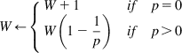
Features of TCP rate control such as Slow Start, additive increase during congestion avoidance, or recovery from lost packets are left unchanged. However, instead of cutting its window size by 2 in response to a marked ACK, DCTCP applies the following rule once every RTT:
(2)
(3)
Thus, a DCTCP sender starts to reduce its window as soon as the queue size exceeds K (rather than wait for a packet loss) and does so in proportion to the average fraction of marked packets. Hence, if very few packets are marked then the window size hardly reduces, and conversely in the worst case if every packet is marked, then the window size reduces by half every RTT (as in Reno).
Following Alizadeh et al. [2,16], we now provide an analysis of DCTCP. It can be shown that in the fluid limit, the DCTCP window size W, the marking estimate ![]() , and the queue size at the bottleneck node b(t) satisfy the following set of delay-differential equations:
, and the queue size at the bottleneck node b(t) satisfy the following set of delay-differential equations:
(4)
(5)
(6)
where p(t) is the marking probability at the bottleneck node and is given by
(7)
T(t) is the round trip latency, C is the capacity of the bottleneck node, and N is the number of DCTCP sessions passing through the bottleneck.
Equations 4 to 6 are equivalent to the corresponding equations 54 and 55 for TCP Reno presented in Chapter 3. Equation 5 can be derived as the fluid limit of equation 1, and equation 6 can be derived from the fact that the data rate for each of the N sessions is given by W(t)/T(t), while C is the rate at which the buffer gets drained. To derive equation 4, note that 1/T(t) is the rate at which the window increases (increase of 1 per round-trip), and ![]() is the rate at which the window decreases when one or more packets in the window are marked (because
is the rate at which the window decreases when one or more packets in the window are marked (because ![]() is the decrease in window size, and this happens once per round trip).
is the decrease in window size, and this happens once per round trip).
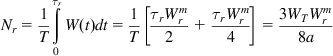
Using the approximation T=D + K/C (where D is the round trip propagation delay), it was shown by Alizadeh et al. [16] that this fluid model agrees quite well with simulations results. Because of the 0-1 type marking function p(t), this system of equations does not have a fixed point and instead converges to a periodic limit-cycle behavior in steady state. It is possible to do a stability analysis of the system using sophisticated tools from Poincare Map theory and thus derive conditions on the parameters C, N, D, K, and g for the system to be stable, which are ![]() and (CD+K)/N>2. They also showed that to attain 100% throughput, the minimum buffer size K at the bottleneck node is given by
and (CD+K)/N>2. They also showed that to attain 100% throughput, the minimum buffer size K at the bottleneck node is given by
(8)
This is a very interesting result if we contrast it with the minimum buffer size required to sustain full throughput for TCP Reno, which from Chapter 2 is given by CD. Hence, DCTCP is able to get to full link utilization using just 17% of the buffers compared with TCP Reno, which accounts for the lower latencies that the flows experience.
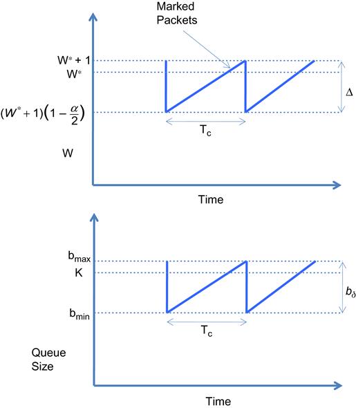
Using a simpler model and under the assumption that all N connections are synchronized with each other, it is possible to obtain expressions for the fluctuation of the bottleneck queue size [2], and we do this next (Figure 7.5). This model, called the Sawtooth model by Alizadeh et al. [16], is of the more traditional type that we have analyzed in previous chapters, and the synchronization assumption makes it possible to compute the steady-state fraction of the packets that are marked at a switch. This quantity is assumed to be fixed, which means that the model is only accurate for small values of the smoothing parameter g.
An analysis of the Sawtooth model is done next:
Let S(W1,W2) be the number of packets sent by the sender while its window size increases from W1 to W2>W1. Note that this takes (W2–W1) round trip times because the window increases by at most 1 for every round trip. The average window size during this time is given by (W1+W2)/2, and because the increase is linear, it follows that
(9)
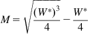
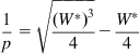
When the window increases to W*=(CD+K)/N, then the queue size reaches K (because CD+K is the maximum number of packets that can be in transit + waiting for service for a buffer size of K and a single source), and the switch starts to mark packets with the congestion codepoint. However, it takes one more round trip delay for this information to get to the source, during which the window size increases to W*+1. Hence, the steady-state fraction of marked packets is given by
(10)
By plugging equations 9 into 10 and simplifying, it follows that
(11)
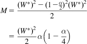
To compute the magnitude of oscillations in the queue size, we first compute the magnitude of oscillations in window size of a single connection, which is given by
(12)
Because there are N flows, it follows that the oscillation in the queue size ![]() , is given by
, is given by
(13)
From equation 13, it follows that the amplitude of queue size oscillations in DCTCP is ![]() , which is much smaller than the oscillations in TCP Reno, which are
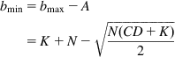
, which is much smaller than the oscillations in TCP Reno, which are ![]() . This allows for a smaller threshold value K, without the loss of throughput. Indeed, the minimum value of the queue size bmin, can also be computed and is given by
. This allows for a smaller threshold value K, without the loss of throughput. Indeed, the minimum value of the queue size bmin, can also be computed and is given by
(14)
 (14)
(14)
To find a lower bound on K, we can minimize equation 14 over N and then choose K so that this minimum is larger than zero, which results in
(15)
which is close to the value 0.17D derived from the more exact analysis by Alizadeh et al. [16].
Simulation results in Alizadeh et al. [2] show that DCTCP achieves its main objective of reducing the size of the bottleneck queue size; indeed, the queue size with DCTCP is 1/20th the size of the corresponding queue with TCP Reno and RED.
Using this model, it is also possible to derive an expression for the average throughput of DCTCP as a function of the packet drop probability, and we do so next. Using the deterministic approximation technique described in Section 2.3 of Chapter 2, we compute the number of packets transmitted during a window increase–decrease cycle M and the length of the cycle ![]() to get the average throughput
to get the average throughput ![]() , so that
, so that
(16)
In this equation, ![]() is the number of round trip latencies in a cycle, and
is the number of round trip latencies in a cycle, and ![]() is approximated by equation 11. Note that M is approximately given by
is approximated by equation 11. Note that M is approximately given by ![]() , so that
, so that
Substituting for ![]() using equation 11, we obtain
using equation 11, we obtain
Following the usual procedure, we equate M=1/p, where p is the packet drop probability, so that
After some simplifications, we obtain
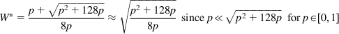
Solving the resulting equation for W*, we obtain
(17)
 (17)
(17)
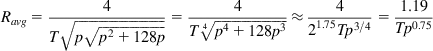
Substituting for M=1/p and W* in equation 16, we obtain
(18)
 (18)
(18)
so that the Response Function for DCTCP is given by (see Chapter 5 for a definition of the Response Function)
(19)
Equation 18 and 19 imply that DCTCP is comparable to high-speed protocols such as High Speed TCP (HSTCP) in being able to use large link capacities in an efficient manner. Unlike HSTCP or CUBIC, DCTCP does not make allowances to be Reno friendly, so there is no cut-off link capacity below which DCTCP behaves like Reno. The higher throughput of DCTCP compared with Reno can be attributed to DCTCP’s less drastic reductions in window size on encountering packet drops. The exponent d of the packet drop probability is given by d=0.75, which points to high degree of intraprotocol RTT unfairness in DCTCP. However Alizadeh et al. [2] have shown by simulations that the RTT unfairness in DCTCP is actually close to that of Reno with RED. Hence, the unfairness predicted by equation 18 is an artifact of the assumption that all the N sessions are synchronized in the Sawtooth model.
7.3.1 The HULL Modification to Improve DCTCP
Alizadeh et al. [4], in a follow-on work, showed that it is possible to reduce the flow latencies across a DCN even further than DCTCP by signaling switch congestion based on link utilizations rather than queue lengths. They came up with an algorithm called HULL (High bandwidth Ultra Low Latency), which implements this idea and works as follows:
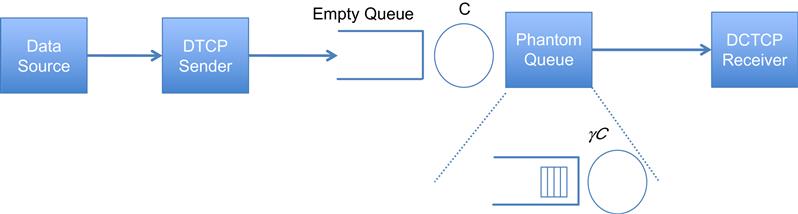
Consider a simulated queue called Phantom Queue (PQ), which is a virtual queue associated with each switch egress port, and in series with it as shown in Figure 7.6 (sometimes it is also called a Virtual Out Queue [VOQ]). Note that the PQ is not really a queue because it does not store packets; however, it is simply a counter that is updated as packets exit the link to determine the queuing that would have occurred on a slower virtual link (typically about 10% slower). It then marks the ECN for packets that pass through it when the simulated queue is above a fixed threshold. The PQ attempts to keep the aggregate transmission rate for the congestion-controlled flows to be strictly less than the link capacity, which keeps the switch buffers mostly empty. The system also uses DCTCP as its congestion control algorithm to take advantage of its low latency properties.
To further reduce the queue build-up in the switches, HULL also implements Packet Pacing at the sender. The pacer should be implemented in hardware in the server Network Interface Card (NIC) to smooth out the burstiness caused by the data transfer mechanism between the main memory and the NIC.
As a result of these enhancements, HULL has been shown achieve 46% to 58% lower average latency compared with DCTCP, and 69% to 78% slower 99th percentile latency.
7.4 Deadline-Aware Congestion Control Algorithms
Section 7.2.1 showed that flows in DCNs come with real-time constraints on their completion times, typically of the order of tens of milliseconds. One of the issues with DCTCP is that it does not take these deadlines into account; instead, because of its TCP heritage, it tries to assign link bandwidth fairly to all flows irrespective of their deadlines. As a result, it has been shown [5] that as much as 7% of flows may miss their deadlines with DCTCP. A number of recent DCN congestion control proposals seek to address this shortcoming. All of them try to incorporate the flow deadline information into the congestion control algorithm in some way and in the process have a varying impact on the implementation at the sender, the receiver, and the switches. In this subsection, we will describe two of these algorithms, namely, Deadline Aware Datacenter TCP (D2TCP) [3] and D3 [5], in order of increasing difference from the DCTCP design.
7.4.1 Deadline Aware Datacenter TCP
Historically, the D3 algorithm came first, but we will start with D2TCP because it is closer in design to DCTCP and unlike D3 does not impact the switches or make fundamental changes to TCP’s additive increase/multiplicative decrease (AIMD) scheme. In fact, just like DCTCP, it is able to make use of existing ECN-enabled Ethernet switches.
The basic idea behind D2TCP is to modulate the congestion window size based on both deadline information and the extent of congestion. The algorithm works as follows:
• As in DCTCP, each switch marks the CE bit in a packet if its queue size exceeds a threshold K. This information is fed back to the source by the receiver though ACK packets.
• Also as in DCTCP, each sender maintains a weighted average of the extent of congestion ![]() , given by
, given by
(20)
where F is the fraction of marked packets in the most recent window and g is the weight given to new samples.
• DCTCP introduces a new variable that is computed at the sender, called the deadline imminence factor d, which is a function of a flows deadline value, and such that the resulting congestion behavior allows the flow to safely complete within its deadline. Define Tc as the time needed for a flow to complete transmitting all its data under a deadline agnostic behavior, and ![]() as the time remaining until its deadline expires. If
as the time remaining until its deadline expires. If ![]() , then the flow should be given higher priority in the network because it has a tight deadline and vice versa. Accordingly, the factor d is defined as
, then the flow should be given higher priority in the network because it has a tight deadline and vice versa. Accordingly, the factor d is defined as
(21)
Note that ![]() is known at the source. To compute Tc, consider the following: Let X be the amount of data (in packets) that remain to be transmitted and let Wm be the current maximum window size. Recall from Section 7.3 that the number of packets transmitted per window cycle N is given by
is known at the source. To compute Tc, consider the following: Let X be the amount of data (in packets) that remain to be transmitted and let Wm be the current maximum window size. Recall from Section 7.3 that the number of packets transmitted per window cycle N is given by
so that ![]()
Hence, the number round trip latencies M in a window increase–decrease cycle is given by
Again from Section 7.3, the length ![]() of a cycle is given by
of a cycle is given by
where T=D + K/C. It follows that Tc is given by
so that
(22)
• Based on ![]() and d, the sender computes a penalty function p applied to the window size, given by
and d, the sender computes a penalty function p applied to the window size, given by
(23)
The following rule is then used for varying the window size once every round trip
(24)
 (24)
(24)
When ![]() then p=0, and the window size increases by one on every round trip. At the other extreme, when
then p=0, and the window size increases by one on every round trip. At the other extreme, when ![]() , then p=1, and the window size is halved just as in regular TCP or DCTCP. For
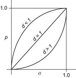
, then p=1, and the window size is halved just as in regular TCP or DCTCP. For ![]() , the algorithm behaves differently compared with DCTCP, and depending on the value of d, the window size gets modulated as a function of the deadlines. In Figure 7.7, we plot p as a function of
, the algorithm behaves differently compared with DCTCP, and depending on the value of d, the window size gets modulated as a function of the deadlines. In Figure 7.7, we plot p as a function of ![]() , for d<1, d=1 and d>1. Note than when d=1, then
, for d<1, d=1 and d>1. Note than when d=1, then ![]() , so that the system matches DCTCP. If d>1, then from equation 21, it follows that the time required to transmit the remaining data is larger than allowed by the deadline; hence, the flow should be given higher priority by the network. Equation 23 brings this about by reducing the value of p for such a flow, resulting in a larger window size by equation 24. Conversely, if d<1, equation 24 leads to a smaller window size and hence lower priority for the flow. Hence, the net effect of these window change rules is that far-deadline flows relinquish bandwidth so that near-deadline flows can have greater short-term share to meet their deadlines. If the network congestion keeps increasing despite the far-deadline flows backing off, then Figure 7.7 shows that the curves for d<1 converges toward that for d>1, which implies that in this situation even the near-deadline flows reduce their aggressively.
, so that the system matches DCTCP. If d>1, then from equation 21, it follows that the time required to transmit the remaining data is larger than allowed by the deadline; hence, the flow should be given higher priority by the network. Equation 23 brings this about by reducing the value of p for such a flow, resulting in a larger window size by equation 24. Conversely, if d<1, equation 24 leads to a smaller window size and hence lower priority for the flow. Hence, the net effect of these window change rules is that far-deadline flows relinquish bandwidth so that near-deadline flows can have greater short-term share to meet their deadlines. If the network congestion keeps increasing despite the far-deadline flows backing off, then Figure 7.7 shows that the curves for d<1 converges toward that for d>1, which implies that in this situation even the near-deadline flows reduce their aggressively.
Vamanan et al. [3] simulated D2TCP and showed that the algorithm reduces the fraction of missed deadlines by 75% when compared to DCTCP and 50% compared with D3. It is also able to coexist with TCP flows without degrading their performance.
7.4.2 The D3 Algorithm
Both the DCTCP and D2TCP algorithms are designed to make use of regular Ethernet switches, albeit those that support RED. In this section, we describe the D3 algorithm that requires significantly enhanced switch functionalities [5]. D3 was the first algorithm that attempted to directly adapt the classical EDF scheduling algorithm to DCNs, and later another algorithm called PDQ [6] built upon it to significantly and improved its performance by adding preemptive scheduling of flows. Indeed, both of these algorithms take us out of the province of AIMD-type window increment–decrement algorithms that have dominated congestion control designs since the 1980s. Note that both of these algorithms are based on the use of First In First Out (FIFO) scheduling at the network nodes. These algorithms are able to simulate the effect of node level EDF scheduling by controlling the rate (in D3) or the admission of packets into the network (in PDQ).
A traditional EDF scheduler operates as follows: All packets arriving into the queue carry an extra piece of information in their headers, which is the deadline by which they have to be finish transmission. The EDF scheduler prioritizes transmissions, such that packets with the smallest or earliest deadline are transmitted first. EDF scheduling can be done either on a nonpreemptive or preemptive basis. In nonpreemptive scheduling, after a transmission is started, it finishes to completion; in preemptive scheduling, a packet with a smaller deadline can preempt the transmission of a packet with a longer deadline. A preemptive EDF scheduler can be proven to be optimal [17] in the sense that if the link utilization is under 100%, then all packets under EDF scheduling will meet their deadlines.
A straightforward application of EDF to a DCN runs into the following problems: (1) It is difficult to do EDF on a packet-by-packet basis at switches because packets do not carry any information about their deadlines, and (2) DCN switches do not incorporate priority-based transmission such that packets with closer deadlines could be transmitted earlier. The D3 algorithm solves the first problem by assigning deadlines on a flow basis rather than on a packet basis. Furthermore, it solves the second problem by translating the flow deadline requirement into an equivalent bandwidth requirement, and then reserving this bandwidth, on a per round trip basis at all switches along the path. PDQ, on the other hand, attaches extra fields to the packet header with information about flow deadlines and size among other quantities and lets the switches make priority decisions regarding the flows, which are communicated back to the sources.
We now provide a brief description of the D3 algorithm:
• Applications communicate their size and deadline information when initiating a flow. The sending server uses this information to request a desired rate r given by r=s/d, where s is the flow size and d is the deadline. Note that both s and d change as a flow progresses, and these are update by the sender.
• The rate request r is carried in the packet header as it traverses the switches on its path to the receiver. Each switch assigns an allocated rate that is fed back in the form of a vector of bandwidth grants to the sender though an ACK packet on the reverse path. Note that a switch allocates rates on an First Come First Served (FCFS) basis, so that if it has spare capacity after satisfying rate requests for all the deadline flows, then it distributes it fairly to all current flows. Hence, each deadline flow gets allocated a rate a, where a=r + fs and fs is the fair share of the spare capacity (Note that fs can be computed using the techniques described for the RCP algorithm in Chapter 5.)
• On receiving the ACK, the source sets the sending rate to the minimum of the allocated rates. It uses this rate for a RTT (rather than using an AIMD-type algorithm to determine the rate) while piggybacking a rate request for the next RTT on one of the data packets. Note that D3 does not require a reservation for a specific sending rate for the duration of the entire flow, so the switches do not have to keep state of their rate allocation decisions. Also, D3 does not require priority scheduling in the switches and can work with FIFO scheduled queues.
The D3 protocol suffers from the following issues:
• Because switches allocate bandwidth on a FCFS basis, it may result in bandwidth going to flows whose deadlines are further away but whose packets arrive at the switch earlier. It has been shown [3] that this inverts the priorities of 24% to 33% of requests, thus contributing to missed deadlines.
• D3 requires custom switching sets to handle requests at line rates, which precludes the use of commodity Ethernet switches.
• It is not clear whether the D3 rate allocation strategy can coexist with legacy TCP because TCP flows do not recognize D3’s honor based bandwidth allocation. This means that a TCP flow can grab a lot of bandwidth so that the switch will not be able to meet the rate allocation promise it made to a D3 source.
The PDQ [6] scheduler was designed to improve upon D3 by providing a distributed flow scheduling layer, which allows for flow preemption, while using only FIFO tail-drop queues. This, in addition to other enhancements, improves the performance considerably, and it was shown that PDQ can reduce the average flow completion time compared with TCP and D3 by 30% and can support three times as many concurrent senders as D3 while meeting flow deadlines. PDQ is able to implement sophisticated strategies such as EDF or SJF (Shortest Job First) in a distributed manner, using only FIFO drop-tail queues, by explicitly controlling the flow sending rate and retaining packets from low-priority flows at senders.
7.5 Load Balancing over Multiple Paths with Multipath TCP (MPTCP)
One of the features that differentiates a DCN from other types of networks is the presence of multiple paths between end points. As explained in Section 7.2, these multiple paths are integral to realizing the full bisection bandwidth between servers in DCN architectures such as a Clos-based Fat Tree or VL2 networks. To accomplish this, the system should be able to spread its traffic among the multiple paths while at the same time providing congestion control along each of the paths.
The traditional way of doing load balancing is to do it on a flow basis, with each flow mapped randomly to one of the available paths. This is usually done with the help of routing protocols, such as ECMP, that use a hash of the address, port number and other fields to do the randomization. However, randomized load balancing cannot achieve the full bisectional bandwidth in most topologies because often a random selection causes a few links to be overloaded and other links to have little load. To address this issue, researchers have proposed the use of centralized schedulers such as Hedera [18]. This algorithm detects large flows, which are then assigned to lightly loaded paths, while existing flows may be reassigned to maximize overall throughput. The issue with centralized schedulers such as this is that the scheduler has to run often (100 ms or faster) to keep up with the flow arrivals. It has been shown by Raiciu et al. [9] that even if a scheduler runs every 500 ms, its performance is no better than that of a randomized load-balancing system.
To address these shortcomings in existing load balancers, Raiciu et al. [9] and Wischik et al. [10] designed a combined load-balancing plus congestion control algorithm called Multipath TCP (MPTCP), which is able to establish multiple subflows on different paths between the end systems for a single TCP connection. It uses a simple yet effective mechanism to link the congestion control dynamics on the multiple subflows, which results in the movement of traffic away from more congested paths and on to less congested ones. It works in conjunction with ECMP, such that if ECMP’s random selection causes congestion along certain links, then the MPTCP algorithm takes effect and balances out the traffic.
The MPTCP algorithm operates as follows:
• MPTCP support is negotiated during the initial SYN exchange when clients learn about additional IP addresses that the server may have. Additional subflows can then be opened with IP addresses or in their absence by using different ports on a single pair of IP addresses. MPTCP then relies on ECMP routing to hash the subflows to different paths.
• After the multiple subflows have been established, the sender’s TCP stack stripes data across all the subflows. The MPTCP running at the receiver reconstructs the receive data in the original order. Note that there is no requirement for an application to be aware that MPTCP is being used in place of TCP.
• Each MPTCP subflow have its own sequence space and maintains its own congestion window so that it can adapt independently to conditions along the path. Define the following:
Wr: Window size for the rth subflow
The following window increment–decrement rules are used by MPTCP:
For each ACK received on path r, increase the window as per
(25)
where
(26)
 (26)
(26)
On detecting a dropped packet on subflow r, decrease its window according to
(27)
Hence, MPTCP links the behavior of the subflows by adapting the additive increase constant. These rules enable MPTCP to automatically move traffic from more congested paths and place it on less congested ones. Wischik et al. [10] used heuristic arguments to justify these rules, which we explain next:
• Note that if the TCP window is increased by a/W per ack, then the flow gets a window size that is proportional to ![]() (see equation 68 in Section 2.3.1 of Chapter 2). Hence, the most straightforward way to split up the flows is by choosing
(see equation 68 in Section 2.3.1 of Chapter 2). Hence, the most straightforward way to split up the flows is by choosing ![]() and assuming equal round trip delays, resulting in an equilibrium window size of W/n for each subflow. However, this algorithm can result in suboptimal allocations of the subflows through the network because it uses static splitting of the source traffic instead of adaptively trying to shift traffic to routes that are less congested.
and assuming equal round trip delays, resulting in an equilibrium window size of W/n for each subflow. However, this algorithm can result in suboptimal allocations of the subflows through the network because it uses static splitting of the source traffic instead of adaptively trying to shift traffic to routes that are less congested.
• Adaptive shifting of traffic to less congested routes can be done by the using the following rules:
(28)
(29)
Consider the case when the packet drop rates are not equal. As a result of equations 28 and 29, the window increment and decrement amounts are the same for all paths; hence, it follows that the paths with higher drop rate will see more window decreases, and in equilibrium, the window size on these paths will go to zero.
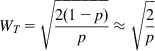
Assuming that each of the paths have the same packet loss rate p and using the argument that in equilibrium, the increases and decreases of the window size must balance out, it follows that
(30)
so that
(31)
 (31)
(31)
It follows that the total window size WT, is the same as for the case when all the traffic was carried on a single path. Hence, unlike the case of static splitting, the adaptive splitting rule does not use more bandwidth by virtue of the fact that it is using multiple paths.
• The window increment–decrement rules (equations 28 and 29) lead to the situation where there is no traffic directed to links with higher packet drop rates. If there is no traffic going to a path for a subflow, then this can be a problem because if the drop rate for that link decreases, then there is no way for the subflow to get restarted on that path. To avoid this, it is advisable to have traffic flow even on links with higher loss rates, and this can be accomplished by using the following rules:
(32)
(33)
Note that equation 33 causes a decrease in the rate at which the window decreases for higher loss rate links, and the factor a in equation 32 increases the rate of increase. We now derive an expression for Wr for the case when the packet drop rates are different but the round trip latencies are same across all flows.
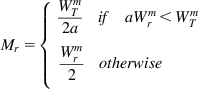
![]() : Maximum window size for the rth subflow
: Maximum window size for the rth subflow
![]() : Length of a window increase–decrease cycle for the rth subflow
: Length of a window increase–decrease cycle for the rth subflow
Mr: Multiple of RTTs contained in an increase–decrease cycle
Nr: Number of packets transmitted an increase–decrease cycle for the rth subflow
We will use the fluid flow model of the system (see Section 7.3). Because the window size increases by aWr/WT for every RTT and the total increase in window size during a cycle is Wr/2, it follows that
so that
Also
(34)
 (34)
(34)
Using the deterministic approximation technique, it follows that
(35)
From equation 35, it follows that
(36)
Substituting equation 36 back into equation 35, we finally obtain
(37)
 (37)
(37)
Hence, unlike the previous iteration of the algorithm, this algorithm allocates a nonzero window size to flows with larger packet drop rates.
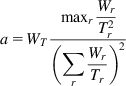
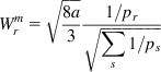
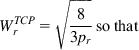
• The window increment–decrement rules (equations 32 and 33) are effective in guiding traffic toward links with lower loss rates; however, they do not work very well if the paths have differing round trip delays. This is because the path with the higher round trip delay will experience a lower rate of increase of window size, resulting in a lower throughput even if the packet loss rates are the same. Wischik et al. [10] solved this problem as follows: First, they noted that if
(38)
is satisfied, where ![]() is the window size attained by a single-path TCP experiencing path r’s loss rate, then we can conclude the following: (1) The multipath flow takes at least as much capacity as a single path TCP flow on the best of the paths, and (2) the multipath flow takes no more capacity on any single path (or collection of paths) than if it was a single path TCP using the best of those paths. They also changed the window increment–decrement rules to the following:
is the window size attained by a single-path TCP experiencing path r’s loss rate, then we can conclude the following: (1) The multipath flow takes at least as much capacity as a single path TCP flow on the best of the paths, and (2) the multipath flow takes no more capacity on any single path (or collection of paths) than if it was a single path TCP using the best of those paths. They also changed the window increment–decrement rules to the following:
(39)
(40)
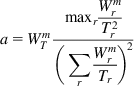
where a is given by
(41)
 (41)
(41)
The difference between this algorithm and the previous one is that window increase is capped at 1/Wr, which means that the multipath flows can take no more capacity on any path than a single-path TCP flow would.
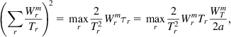
The expression for a in equation 41 can be derived by combining equations 39 and 40 with the condition (equation 38), and we proceed to do this next.
Using the same notation as before, note that the window size for the rth subflow increases by ![]() in each round trip. Hence, it follows that
in each round trip. Hence, it follows that
(42)
 (42)
(42)
It follows that
(43)
Using the deterministic approximation technique, it follows that
(44)
In equation 38, note that
(45)
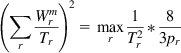 (45)
(45)
Substituting for pr from (44) and ![]() from (43), it follows that
from (43), it follows that
from which (41) follows.
Raiciu et al. [9] have carried out extensive simulations of MPTCP and have shown that it leads to appreciable improvement in DCN performance. For example, for an eight-path Fat Tree CLOS network, regular TCP with an ECMP-type load balancing scheme only realized 50% of the total bandwidth between two servers, but MPTCP with eight subflows realized about 90% of the total bandwidth. Moreover, the use of MPTCP can lead to new interconnection topologies that are not feasible under regular TCP. Raiciu et al. [9] suggested a modified form of Fat Tree, which they call Dual-Homed Fat Tree (DHFT), which requires a server to have two interfaces to the ToR switch. They showed that DHFT has significant benefits over the regular Fat Tree topology.
7.6 The Incast Problem in Data Center Networks
The Incast problem in DCNs is caused by the temporal dependency created on message traffic that is generated as a result of the Map-Reduce type parallel execution illustrated in Figure 7.4. The parent node sends queries in parallel to multiple leaf nodes, and the subsequent responses from the leaf nodes also tend to be bunched together, as shown in Figure 7.8. This pattern is referred to as Incast [19,20].
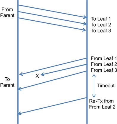
The response size not very large on the average, usually a few kilobytes, but even then it has been observed that they suffer from a large packet loss rate. The reason for this has to do with the hardware design of the DCN switches, which tend to have shallow buffers, which are shared among all the ports in switch. As a result, the Incast pattern can lead to a packet drop in one of the following scenarios: (1) because of multiple query responses overflowing a port buffer, (2) because of buffer exhaustion as a result of long background flows on the same port as the Incast packets, and (3) because of buffer exhaustion as a result of long background flows on a different port than the Incast packets.
To solve the Incast problem, researchers do one of the following: (1) try to avoid packet loss or reduce the rate of packet loss or (2) quickly recover from lost packets.
In the first category are techniques such as increasing the switch buffer size and adding a random delay to query responses from the leaf nodes. The latter technique reduces the occurrence of Incast-generated timeouts but at the cost of an increase in the median Job response time. The use of a DCN-specific congestion control protocol such as DCTCP also falls in this category because they are mode effective in keeping buffer occupancy low compared with regular TCP. In the second category are techniques such as reducing the TCP packet lost timer RTO from the default value of a few 100 ms to less than 1 ms. This has been very effective in improving Incast performance.
7.7 Further Reading
Congestion control in DCNs is an extremely active area, with researchers exploring new ideas without being constrained by legacy compatibility issues. One such idea is that of in-network congestion control in which the switches bear the burden of managing traffic. The justification for this is that traditional TCP congestion control requires at least one RTT to react to congestion that is too slow for DCNs because congestion builds very quickly, in less than RTT seconds. The in-network schemes go hand in hand with the multipath nature of modern datacenter architecture, and a good example of this category is the Detail protocol [7]. Routing within the network is done on a packet-by-packet basis and is combined with load balancing, such that a packet from an input queue in a switch is forwarded to the output interface with the smallest buffer occupancy (thus taking advantage of the fact that there are multiple paths between the source and destination). This means that packets arrive at the destination out of order and have to be resequenced before being delivered to the application. This mechanism is called Adaptive Load Balancing (ALB). Furthermore, if an output queue in a switch is congested, then this may result in input queues becoming full as well, at which point the switch backpressures the upstream switch by using the IEEE 802.1Qbb Priority based Flow Control (PFC) mechanism.
The pFabric [8] is another protocol with highly simplified end system algorithm and with the switches using priority-based scheduling to reduce latency for selected flows. Unlike in D2TCP, D3 or PDQ, pFabric decouples flow priority scheduling from rate control. Each packet carries its priority in its header, which is set by the source based on information such the deadline for the flow. Switches implement priority-based scheduling by choosing the packet with the high priority number for transmission. If a packet arrives to a full buffer, then to accommodate it, the switch drops a packet whose priority is lower. pFabric uses a simplified form of TCP at the source without congestion avoidance, fast retransmits, dupACKs, and so on. All transmissions are done in the Slow Start mode, and congestion is detected by the occurrence of excessive packet drops, in which case the system enters into probe mode in which it transmits minimum size packets. Hence, pFabric does away with the need to do adaptive rate (or window) control at the source.
Computing services such as Amazon EC2 are a fast-growing category of DCN applications. These systems use Virtual Machines (VMs), which share the servers by using a Processor Sharing (PS) type scheduling discipline to make more efficient use of the available computing resources. Wang and Ng [21] studied the impact of VMs on TCP performance by using network measurements and obtained some interesting results: They found out that PS causes a very unstable TCP throughput, which can fluctuate between 1 Gbps and 0 even at about tens of milliseconds in granularity. Furthermore, even in a lightly congested network, they observed abnormally large packet delay variations, which were much larger than the delay variations caused by network congestion. They attributed these problems to the implementation of the PS scheduler that is used for scheduling VMs. They concluded that TCP models for applications running on VMs should incorporate an additional delay in their round trip latency formula (i.e., the delay caused by end host virtualization).