Congestion Control in Ethernet Networks
This chapter is on the topic of congestion control in Ethernet networks. Traditionally, Ethernet, which operates at Layer 2, has left the task of congestion control to the TCP layer. However, recent developments such as the spread of Ethernet use in applications such as Storage Area Networks (SANs) has led the networking community to revisit this design because SANs have a very strict requirement that no packets be dropped. As a result, the Institute of Electrical and Electronics Engineers (IEEE) 802.1 Standards group has recently proposed a congestion control algorithm called IEEE802.1Qau or Quantum Congestion Notification (QCN) for use in Ethernet networks. This algorithm uses several advances in congestion control techniques described in the previous chapters, such as the use of rate averaging at the sender and Active Queue Management (AQM) feedback, which takes the occupancy as well as the rate of change of the buffer size into account.
Keywords
Ethernet congestion control; Quantum Congestion Notification; QCN; Reaction Point or RP algorithm; Control Point or CP Algorithm; QCN Stability Analysis; IEEE802.1Qau
8.1 Introduction
Ethernet is the most prevalent Layer 2 technology used in Internet Protocol (IP) networks; it is almost as old as IP itself. Traditionally, Ethernet left the job of congestion control to IP while providing basic medium access control (its original purpose in shared media links) and later Layer 2 bridging and switching functionalities. This state of affairs started to change in the past 10 to 15 years as the use of Ethernet expanded to wider domains. One of these domains is data center networking, and Chapter 7 discusses server-to-server networking in DCNs using Ethernet as the switching fabric with TCP running on top.
An aspect of data center networks (DCNs) not discussed in Chapter 7 is that of communications between the servers and storage devices. The networks that are used to interconnect them together are known as Storage Area Networks (SANs). Fiber Channel (FC) is a Layer 1–2 high-speed point-to-point interconnect technology that is used to create SANs. A very strong requirement in SAN networks is that the packet drop rate caused by buffer overflows should be zero. FC networks use a hop-by-hop congestion control method to accomplish this goal, whereby a node that is running out of buffers sends a signal to the node upstream from it to stop it from transmitting.
Link speeds in FC increased over time, but they were not able to keep pace with the more rapid increases in Ethernet link speeds that have gone from 1 to 10 Gbps and then to 100 Gbps in the past decade and a half. In addition, Ethernet adaptors and switches come at a lower cost because of their wider adoption in the industry. Motivated by these considerations, the industry created a FC over Ethernet (FCoE) standard, in which Ethernet is used as the Layer 1–2 substrate in SANs. However, using TCP as the congestion control mechanism will not work in an FCoE SAN because TCP does drop packets during the course of its normal operation. As a result, an effort was started in the Institute of Electrical and Electronics Engineers (IEEE) 802.2 Standards Body to make modifications to Ethernet so that it is suitable for deployment in a SAN (or a DCN in general), called Data Center Bridging (DCB) [1]. One of the outcomes of this effort is a congestion control protocol called IEEE 802.1Qau [2], also known as Quantum Congestion Notification (QCN), which operates at the Ethernet layer and aims to satisfy the special requirements in DCB networks [3].
There is more design latitude in the design of QCN compared with TCP because Ethernet provides 6 bits of congestion feedback (as opposed to 1 bit in TCP), and the QCN design takes advantage of this by implementing a proportional-integral (PI) controller at the Ethernet switch, which we know to be superior than Random Early Detection (RED) controllers. The QCN increase–decrease protocol has some novel features described in Section 8.4. Alizadeh et al. [4] carried out a comprehensive control theoretic analysis of the fluid model of the QCN algorithm that forms the subject matter of Section 8.5.
8.2 Differences between Switched Ethernet and IP Networks
Alizadeh et al. listed the following contrasts between switched Ethernet networks and IP networks [3]. We already mentioned one of them in the Introduction (i.e., packets should not be dropped); the others are:
• Ethernet does not use per-packet ACKs: This means that (1) packet transmissions are not self-clocked, (2) round trip latencies are unknown, and (3) congestion has to be signaled directly by the switches back to the source.
• There are no Packet Sequence Numbers in Ethernet.
• Sources start at Line Rate because there is no equivalent of the TCP Slow-Start mechanism. Because Ethernet implements its congestion control in hardware, a Slow-Start–like algorithm would have required a rate limiter, which are few in number and used up by the main congestion control algorithm.
The next three differences are more specific to DCNs in general and served as constraints in the design of a transport level congestion control algorithm as well:
• Very shallow buffers: Ethernet switch buffers are of the order of 100s of kilobytes in size.
• Small number of simultaneously active connections.
• Multipathing: Traditional Layer 2 networks used Spanning Trees for routing, which restricted the number of paths to one. The use of Equal Cost Multi-Path (ECMP) opens up the system to using more than 1 path.
8.3 Objectives of the Quantum Congestion Notification Algorithm
The QCN algorithm was designed based on all the learning from the design and modeling of TCP congestion control algorithms over the previous 2 decades. As a result, it incorporates features that keep it from falling into performance and stability traps that TCP often runs into. Some of the objectives that it seeks to satisfy include the following:
• Stability: We will use this term in the same sense as in the rest of this book, that is, the bottleneck queue length in a stable system should not fluctuate widely, thus causing overflows and underflows. Whereas the former leads to excessive packet drops, the latter causes link underutilization.
• Responsiveness to link bandwidth fluctuations
• Implementation simplicity: Because the algorithm is implemented entirely in hardware, simplicity is a must.
8.4 Quantum Congestion Notification Algorithm Description
The algorithm is composed of two main parts: Switch or Control Point (CP) Dynamics and Rate Limiter or Reaction Point (RP) Dynamics.
8.4.1 The Control Point or CP Algorithm
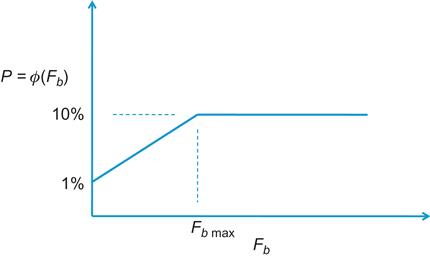
The CP algorithm runs at the network nodes, and its objective is to maintain the node’s buffer occupancy at the operating point beq (Figure 8.1). It computes a congestion measure Fb and randomly samples an incoming packet with a probability that that depends on the severity of the congestion (Figure 8.2). It sends the value of Fb back to the source of the sampled packet after quantizing it to 6 bits.
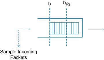
b: Value of the current queue length
bold: Value of the buffer occupancy when the last feedback message was generated
Then Fb is given by the formula:
(1)
where w is a non-negative constant, set equal to 2 for the baseline implementation. Note that equation 1 is basically the PI Active Queue Management AQM controller from Chapter 3. The first term on the RHS is the offset from the target operating point (i.e., the buffer oversubscription), and the second term is proportional to the rate at which the queue size is changing. As per equation 55 in Chapter 3, this is proportional to the difference between the link capacity and the total traffic rate flowing through the link (i.e., the link oversubscription).
When ![]() , there is no congestion, and no feedback messages are sent. When
, there is no congestion, and no feedback messages are sent. When ![]() , then either the buffers or the link or both are oversubscribed, and control action needs to be taken. An incoming packet is sampled with probability
, then either the buffers or the link or both are oversubscribed, and control action needs to be taken. An incoming packet is sampled with probability ![]() (see Figure 8.2), and if ps=1 and
(see Figure 8.2), and if ps=1 and ![]() , then a congestion feedback message is sent back to the source.
, then a congestion feedback message is sent back to the source.
8.4.2 The Reaction Point or RP Algorithm
The RP algorithm runs at the end systems and controls the rate at which Ethernet packets are transmitted in to the network. Unlike TCP, the RP algorithm does not get positive ACKs from the network and hence needs alternative mechanisms for increasing its sending rate. Define the following:
Current rate (RC): The transmission rate of the source
Target rate (RT): The transmission rate of the source just before the arrival of the last feedback message
Byte counter: A counter at the RP for counting transmitted bytes; it is used to time rate increases
Timer: A clock at the RP that is used for timing rate increases. It allows the source to rapidly increase its sending rate from a low value when a lot of bandwidth becomes available.
Initially assuming only the Byte Counter is available, RP uses the following rules for increasing and decreasing its rate.
8.4.2.1 Rate Decreases
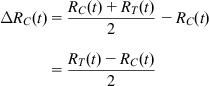
A rate decrease is only done when a feedback message is received, and in this case, CR and TR are updates as follows:
(2)
(3)
The constant Gd is chosen so that ![]() (i.e., the rate can decrease by at most 50%). Because only 6 bits are available for feedback, it follows that
(i.e., the rate can decrease by at most 50%). Because only 6 bits are available for feedback, it follows that ![]() , so that
, so that ![]() accomplishes this objective.
accomplishes this objective.
8.4.2.2 Rate Increases
Rate Increase is done in two phases: Fast Recovery and Active Increase (Figure 8.3)
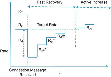
Fast Recovery (FR): The source enters the FR state immediately after a rate decrease event, at which point the Byte Counter is reset. FR consists of 5 cycles, in each of which 150 Kbytes of data are transmitted (100 packets of 1500 bytes each), as counted by the Byte Counter. At the end of each cycle, RT remains unchanged, and RC is updated as follows:
(4)
The rationale behind this rule is if the source is able to transmit 100 packets without receiving another Rate Decrease message (which are sent by the CP once every 100 packets on the average since ps=0.01), then it can conclude that the CP is uncongested, and therefore it increases its rate. Note that FR is similar to the way in which a Binary Increase Congestion Control (BIC) TCP source increases its window size after a packet drop (see Chapter 5). This mechanism was discovered independently by Alizadeh et al. [3].
Active Increase (AI): After 5 cycles of FR, the source enters the AI state, where it probes for extra bandwidth. AI consists of multiple cycles of 50 packets each. During this phase, RT and RC are updates as follows:
(5)
(6)
where RAI is a constant, set to 5 mbps by default.
When RC is extremely small after a rate decrease, then the time required to send out 150 Kbyes can be excessive. To speed this up, the source also uses a Timer, which is used as follows: The Timer is reset when the rate decrease message arrives. The source then enters FR and counts out 5 cycles of T ms duration (T=10 ms in the baseline implementation), and in the AI state, each cycle is T/2 ms long.
• In the AI state, the RC is updated when either the Bye Counter or the Timer completes a cycle.
• The source is in the AI state if and only if either the Byte Counter or the Timer is in the AI state. In this case, when either completes a cycle, RT and RC are updated according to equations 5 and 6.
• The source is in the Hyper-Active Increase (HAI) state if both the Bye Counter and the Timer are in AI. In this case, at the completion of the ith Byte Counter or Timer cycle, RT and RC are updated as follows:
(7)
(8)
where RHAI is set to 50 mbps in the baseline.
8.5 Quantum Congestion Notification Stability Analysis
The stability analysis is done on a simplified model of the type shown in Chapter 3, Figure 3.2, with N connections with the same round trip latency, passing through a single bottleneck node with capacity C [4]. Following the usual recipe, we will first write down the differential equations in the fluid limit and then linearize them around an operating point, which allows us to analyze their stability using tools such as the Nyquist stability criterion. We will assume that ps is fixed at ps=1% in this section to simplify the analysis. Also, all connections are assumed to have the same round trip latency equal to ![]() seconds.
seconds.
In contrast to other congestion control protocols, two variables RC(t) and RT(t), are needed to describe the source behavior:
(9)
(10)
(11)
(12)
(13)
To justify the negative first terms in equations 9 and 10, note that ![]() is the rate at which negative ACKs are arriving at the source. Each of these causes RC to decrease by
is the rate at which negative ACKs are arriving at the source. Each of these causes RC to decrease by ![]() and RT to decrease by
and RT to decrease by ![]() .
.
To derive the positive second term in equation 9, consider the following: The rate RC is increased on the transmission of 150 Kbytes, or 100 packets of 1500 bytes each, if no negative ACK is received in the interim. The change in RC when this happens is given by
To compute the rate at which the RC rate increase events occur, consider the Markov chain in Figure 8.4: It is in state k if k packets have been transmitted back to back without the receipt of a single negative ACK. Starting from state 0, in general, the system may undergo several cycles where it returns back to state 0 before it finally transmits 100 packets back to back and gets to state 100. It can be shown that the average number of packets transmitted to get to state 100 when starting from state 0, is given by
(14)
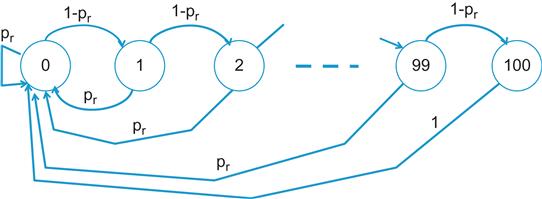
This can be derived as follows: Define ![]() as the average number of packets transmitted to get to state 100 when starting from state i. Based on the Markov chain in Figure 8.4, the sequence ui satisfies the following set of equations (with qr=1−pr):
as the average number of packets transmitted to get to state 100 when starting from state i. Based on the Markov chain in Figure 8.4, the sequence ui satisfies the following set of equations (with qr=1−pr):
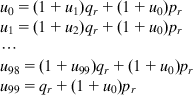
This set of equations can be solved recursively for u0, and results in equation 14.
Because the average time between packet transmissions is given by ![]() , it follows that the average time between increase events is given by
, it follows that the average time between increase events is given by
(15)
The second term on the RHS of equation 9 follows by dividing equation 14 by equation 15. The second term on the RHS of equation 10 is derived using similar considerations. In this case, RT increments by RAI when 500 packets are transmitted back to back without returning to state 0, which results in a Markov chain just like that in Figure 8.4, except that it extends up to state 500.
We now compute the equilibrium values of the variables in equations 9 to 13. In equilibrium, we replace pr by ps throughout.
Define
The fluid flow model in equations 9 to 13 has the following equilibrium points:
(16)
Equation 16 follows by setting db/dt=0 in equation 11.
(17)
Equation 17 follows by setting dRT/dt=0 in equation 10.
Note that from equation 12, it follows that
(18)
and equation 9 implies that
(19)
Substituting for ![]() and
and ![]() from equations 16 and 17 into equation 19, we finally obtain
from equations 16 and 17 into equation 19, we finally obtain
(20)
We now proceed to linearize the equations 9 to 11 around the equilibrium points ![]() . Define the following deltas around the equilibrium:
. Define the following deltas around the equilibrium:
Using the Linearization procedure described in Appendix 3.A of Chapter 3, it can be shown that the following equations result:
(21)
(22)
where
This system of equations can be shown to have the following characteristic function:
(23)
where
(24)
with
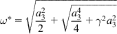
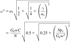
We now state the stability result for QCN. Let
(25)
where
(26)
 (26)
(26)
Then ![]() , and the system in equations 21 and 22 is stable for all
, and the system in equations 21 and 22 is stable for all ![]() .
.
To prove ![]() , note that because
, note that because ![]() , it follows that
, it follows that ![]() .
.
To apply the Nyquist criterion, we pass to the frequency domain and write equation 24 as
where
The last inequality follows from the fact that ![]() , which can verified by substituting
, which can verified by substituting ![]() . Note that setting
. Note that setting ![]() , implies that
, implies that ![]() . Hence, it follows that
. Hence, it follows that ![]() . Because
. Because ![]() is a monotonically decreasing function of
is a monotonically decreasing function of ![]() , it follows that the critical frequency
, it follows that the critical frequency ![]() at which
at which ![]() , is such that
, is such that ![]() . By the Nyquist criterion, if we can show that
. By the Nyquist criterion, if we can show that ![]() for all
for all ![]() , then the system is stable. This can be done as follows:
, then the system is stable. This can be done as follows:
Because ![]() , it follows that
, it follows that
(27)
 (27)
(27)
The last inequality follows from the fact that ![]() . Defining
. Defining
note that ![]() and for
and for ![]() ,
, ![]() . Moreover
. Moreover ![]() is convex for
is convex for ![]() , which implies that
, which implies that ![]() for
for ![]() , and from equation 27, it follows that
, and from equation 27, it follows that ![]() in this range, so that the Nyquist stability criterion is satisfied.
in this range, so that the Nyquist stability criterion is satisfied.
8.5.1 Discussion of the Stability Result
Writing out the formula for ![]() in detail, we get
in detail, we get
(28)
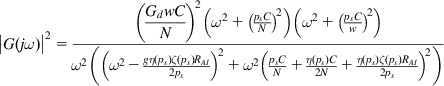 (28)
(28)From equation 28, we can see that the loop gain K for the system is of the order given by
(29)
This is in contrast to TCP Reno (see Chapter 3, Section 3.4), whose loop gain (without RED) is of the order
The absence of the round trip latency from the loop gain in equation 29 is attributable to the fact that QCN is not a window-based congestion control algorithm. In both cases, an increase in link capacity C or a decrease in number of connections drives the system toward instability. Because ![]() , the window based feedback loop plays a role in stabilizing Reno compared with QCN by reducing the system loop gain.
, the window based feedback loop plays a role in stabilizing Reno compared with QCN by reducing the system loop gain.
Also note that the critical frequency can be written as
(30)
 (30)
(30)
It follows that
(31)
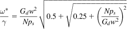 (31)
(31)
(32)
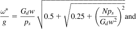 (32)
(32)
(33)
 (33)
(33)
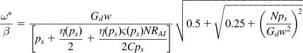
The last two terms in the denominator of equation 33 are much smaller than the first term. As a result, it follows that ![]() , so that the stability threshold for latency is given by
, so that the stability threshold for latency is given by
(34)
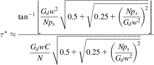 (34)
(34)
Substituting Gd=1/128, w=2 and ps=0.01, we obtain
(35)
and
(36)
Hence, the stability threshold for the round trip latency is inversely proportional to C and directly proportional to ![]() . For example, substituting C=1 Gbps (=83,333 packets/s) and N=10 yields
. For example, substituting C=1 Gbps (=83,333 packets/s) and N=10 yields ![]() .
.
8.6 Further Reading
In addition to QCN, there were two other algorithms that were considered as candidates for the IEEE802.1Qau protocol. The algorithm by Jiang et al. [5] uses an AQM scheme with explicit rate calculation at the network nodes that is fed back to the source. This scheme has some similarities to the RCP algorithm from Chapter 5. The algorithm by Bergamasco and Pan [6] has some similarities to QCN because it is also based on an AQM scheme that provides PI feedback back to the source using a quantized congestion number Fb. The source nodes then use this number to adjust the parameters of their additive increase/multiplicative decrease (AIMD) scheme, such that the rate is additively increased if Fb>0 and multiplicatively decreased if Fb<0.