Congestion Control in Broadband Wireless Networks
This chapter discusses congestion control in broadband wireless networks. This work was motivated by finding solutions to the performance problems that TCP Reno has with wireless links. Because the algorithm cannot differentiate between congestion losses and losses caused by link errors, decreasing the window size whenever a packet is lost has a very detrimental effect on performance. This chapter describes TCP Westwood, which solved this problem by keeping an estimate of the data rate of the connection at the bottleneck node. Thus, when Duplicate ACKs are received, the sender reduces its window size to the transmit rate at the bottleneck node (rather than blindly cutting the window size by half, as in TCP Reno). This works well for wireless links because if the packet was lost because of wireless errors, then the bottleneck rate my still be high, and this is reflected in the new window size. This chapter also describes techniques, such as Split-Connection TCP and Loss Discrimination Algorithms, that are widely used in wireless networks today. The combination of TCP at the end-to-end transport layer and Link Layer Retransmissions (Automatic Retransmissions [ARQ]) or Forward Error Correction (FEC) coding on the wireless link is also analyzed using the results from Chapter 2. The large variation in link capacity that is observed in cellular networks, has led to problem called bufferbloat. We describe techniques using Active Queue Management at the nodes as well as end-to-end algorithms to solve this problem.
Keywords
TCP and wireless systems; congestion control in wireless networks; Split-Connection TCP; ABE; Available Bandwidth Estimator; LDA; Loss Discrimination Algorithm; Zero Receive Window ACK; TCP Westwood; TCP Westwood Plus; TCP and Forward Error Correction (FEC); TCP and ARQ; bufferbloat; Adaptive RED; Controlled Delay (CoDel) AQM; TCP LEDBAT
4.1 Introduction
When users access the Internet using cable, DSL, or wireless mediums, they are doing so over access networks. Over the course of the past 20 years, these networks have been deployed worldwide and today constitute the most common way to access the Internet for consumers. These networks are characterized by transmission mediums such as air, cable, or copper lines, which presented formidable barriers to the reliable transmission of digital data. These problems have been gradually overcome with advances in networking algorithms and physical media modulation technology so that reliable high-speed communication over access networks is a reality today.
In this chapter, the objective is to discuss congestion control over broadband wireless networks. Common examples of broadband wireless networks deployed today include WiFi networks that operate in the unlicensed frequency bands and broadband cellular networks such as 2G, 3G, and LTE that operate in service provider–owned licensed bands. When TCP is used as the transport protocol over these networks, it runs into a number of problems that are not commonly found in wireline networks; some of these are enumerated in Section 4.2. As a result, a lot of effort over the past 10 to 15 years has gone into finding ways in which the wireless medium can be made more data friendly. A lot of this work has gone into improving the wireless physical layer with more robust modulation and more powerful error correction schemes, but equally important have been the advances in the Medium Access Control (MAC) and Transport Layers. Some of this effort has gone into modifying the congestion control algorithm to overcome wireless-related link impairments, and this is the work that described in this chapter.
The fundamental problem that hobbles TCP over wireless links is the fact that it cannot differentiate between congestion and link-error related packet drops. As a result, it reacts to link errors by reducing its transmit window, but the more appropriate reaction would be to retransmit the lost packet. By using the expression for the average TCP throughput that was derived in Chapter 2,

this problem can be solved in several ways:
• By making the wireless link more robust by using channel coding: This leads to a reduction in the wireless link error rate p.
• By retransmitting the lost packets quickly at lower layers of the stack (called Automatic Retransmissions [ARQ]), so that TCP does not see the drops. This also leads to a reduction in p at the cost of an increase in T because of retransmissions.
• By introducing special algorithms at the TCP source that are able to differentiate between congestion drops and link-error related drops. We will discuss one such algorithm called TCP Westwood, which we will show has the same effect on the throughput as a reduction in the link error rate p.
• By splitting the end-to-end TCP connection into two parts, such that the wireless link falls into a part whose congestion control has been specially designed for wireless environments. This technique works because by splitting the connection, we reduce the latency T for each of the resulting two connections. Furthermore, the use of one of the three techniques mentioned above can reduce p.
Modern broadband wireless systems such as LTE have largely solved the link error caused packet drop problem through a combination of strong channel coding and retransmissions. In fact, recent studies of wireless link performance show very few packet losses. However, link errors have been replaced by a new problem in these networks, namely, a large amount of variability in the link latency, leading to a problem that has been christened “bufferbloat.”
The rest of this chapter is organized as follows. In Section 4.2, we introduce the broadband wireless architecture and enumerate the problems that wireless networks present for TCP. In Sections 4.3 and 4.4, we describe several techniques that are used to improve TCP performance in wireless networks, including Split Connections, Bandwidth Estimators, Loss Discrimination Algorithms, and Zero Receive Window (ZRW) ACKs. We illustrate these ideas with a description and analysis of TCP Westwood, which was specifically designed for wireless environments. In Section 4.5, we use the analytical tools developed in Chapter 2 to do performance modeling of TCP running over wireless links that implement techniques such Forward Error Correction (FEC) and Automatic Retransmissions (ARQ) to improve robustness. In Section 4.6, we analyze the bufferbloat issue, its causes, and some of the solutions that have been suggested. Section 4.7 has some useful rules that can be used to test whether link errors are indeed causing packet drops and the effectiveness of various techniques to combat it.
An initial reading of this chapter can be done in the sequence 4.1→4.2→4.3→4.4→4.7 (for those interested in techniques to overcome wireless related link errors) or in the sequence 4.1→4.2→4.6→4.7 (for those interested in the bufferbloat problem and its solutions). Section 4.5 has more advanced material on the analysis of FEC and ARQ algorithms.
4.2 Wireless Access Architecture and Issues
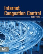
Figure 4.1 is a simplified picture of typical cellular network architecture. Mobile users are connected to a base station unit over a shared wireless connection, and their traffic is backhauled to a wireless gateway, which serves as the demarcation point between the cellular network and the rest of the Internet. The cellular base station is responsible for transforming the digital signal into an analogue waveform for over-the-air transmission, as well as for efficiently sharing the shared wireless medium among multiple users. Modulation techniques have improved over the years, and today both WiFi and LTE networks use an algorithm called OFDMA (orthogonal frequency-division multiplexing). OFDMA is extremely robust against multipath fading, which is the main cause of signal distortion in cellular wireless. All traffic going to the mobiles is constrained to pass through the gateway, which is responsible for higher level functions such as enabling user mobility between base stations and user authentication, sleep mode control, and so on. This gateway is called a packet gateway (PGW) in LTE networks, and Gateway GPRS Support Node (GGSN) or Packet Data Serving Node (PDSN) in 3G networks.
Some of the issues that cause performance problems for TCP in wireless networks are the following:
• Higher link error rates: This has traditionally been the biggest problem with wireless networks and is caused by difficult propagation conditions in the air, leading to high link attenuations and multipath creating reflections from surrounding objects. With the improvement in modulation and network coding techniques over the past 20 years, the error rates have decreased significantly, but they are still much higher compared with wired transmission mediums.
• High link latency: Higher link latency in access networks is partially caused by the physical layer technology used to overcome wireless medium–related transmission problems. A good example of this coding technology is FEC, which helps to make the medium more reliable but leads to higher latency. Also, the MAC layer algorithm operating on top of the physical layer, which is used to share the access medium more efficiently and provide quality of service (QoS) guarantees, introduces latencies of its own. This problem was particularly onerous in the first generation cellular data networks, namely GPRS, which had link latencies of the order of 1 second or more. The latency decreased to about 100 ms in 3G networks and is about 50 ms in LTE. This is still a fairly large number considering that coast-to-coast latency across the continental United States is about 23 ms.
• Large delay variations: This is common in wireless cellular networks and is caused by the base station adapting its physical layer transmission parameters such as modulation and coding, as a function of link conditions, on a user by user basis. This causes the effective channel capacity to fluctuate over a wide range, leading to a phenomenon called bufferbloat. This is caused by the fact the TCP window can never be perfectly matched with the varying link capacity, and at times when the capacity is low and the window is much bigger, the buffer occupancy increases, as shown in Chapter 2.
• Random disconnects: This problem can be caused by one of several reasons. For example, mobile users are momentarily disconnected from the network when they are doing hand-offs between cells. Alternatively, if the wireless signal fades because of multipath or gets blocked because of an obstruction, then it can cause a temporary disconnect. During this time, the TCP source stops receiving ACKs, and if the disconnect time is of the order of 100s of milliseconds, the retransmission timer expires, thus affecting TCP throughput.
• Asymmetric link capacities: Wired mediums are full duplex and have symmetric bandwidth, neither of which is true for wireless access networks. Networks such as Asymmetric Digital Subscriber Loop (ADSL) and Cable Hybrid Fiber Coax (HFC) posses much more capacity in the downlink direction compared with the uplink, and this is also true for cellular wireless. This problem has lessened with the introduction of newer technologies, but it still cannot be ignored. When the uplink has much lower bandwidth compared with the downlink, then the inter-ACK time interval is no longer a good estimate of the bandwidth of the downlink bottleneck capacity; hence, TCP’s self-clocking mechanism breaks down. The analysis in Chapter 2 has been extended to asymmetric links by Lakshman and Madhow [1] and Varma [2].
4.3 Split-Connection TCP
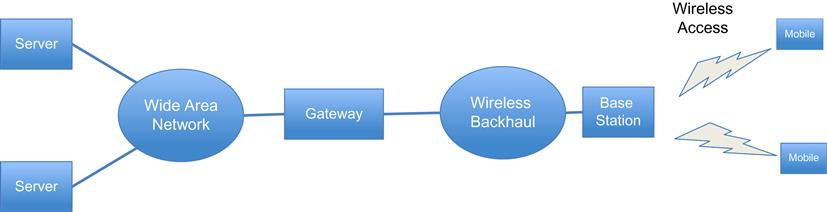
This section describes and analyzes Split-Connection TCP. This is not a new congestion control algorithm but a way to change the structure of the congestion control system so that the problematic part of the network can be isolated. This is done by abandoning the end-to-end nature of the TCP transport layer in favor of multiple TCP-controlled segments in series (Figure 4.2).
As shown, the end-to-end connection traverses two segments in series, the wide area network (WAN) network and the wireless network, with the gateway node that was introduced in Section 4.2 at the boundary between the two. The TCP connection from a server in the WAN to a mobile client is split into two parts, with the first TCP connection (called TCP1) extending from the server to the gateway, and the second TCP connection (called TCP2) extending from the gateway to the client node. The system operates as follows:
• When the server initiates a TCP connection with a client, the connection set-up message is intercepted by the gateway, which then proceeds to do the following: (1) reply to the connection set-up back to the server, as if it were the client, thus establishing the TCP1 connection, and (2) establish the TCP2 connection with the client, with itself as the end point.
• During the data transfer phase of the connection, the gateway intercepts all packets coming from the server over TCP1 and immediately ACKs them back. At the same time, it forwards the packet on TCP2 to the client and discards it after it receives the corresponding ACK from the client.
• If the TCP2 is operating at a slower speed than TCP1, then the data buffers in the gateway start to fill up, and the gateway then proceed to backpressure the server by reducing the size of the receive window in TCP1’s ACK packets.
The design described differs from the one in the original paper on split TCP [3] in the following way: Bakre and Badrinath assumed that the TCP connection would be split at the wireless base station rather than at the gateway. Doing so introduces some additional complications into the design because if the mobile client moves from one base station to another, then the entire state information about the connection and the buffered packets have to be transferred to the new base station. In the design shown in Figure 4.2, on the other hand, this situation is avoided because the split happens at the gateway node, which remains the same even as the client changes base stations.
The benefits of a split-connection TCP design are the following:
• The TCP congestion control algorithms operating on each segment of the network can be tailored to the specific characteristics of the network. The core network is typically constructed from highly reliable optical connections and hence has very low link error rates. The access network, on the other hand, may present several transmission-related problems that were described earlier. As a result, the congestion control algorithm over the wireless network can be specially tailored to overcome these link problems. Note that this can be done without making any changes to TCP1, which is typically running on some server in the Internet and hence cannot be modified easily
• Because of the way that TCP throughput varies as a function of the round trip latency and link error rates, the split-connection design can result in a significant boost to the throughput even in the case in which legacy TCP is used on both connections. This claim is proven below.
Rns: Throughput of the end-to-end non-split TCP connection
Rsp: End-to-end throughput for the split-TCP connection
R1: Throughput of TCP1 in the split-connection case
R2: Throughput of TCP2 in the split-connection case
T: Round trip latency for the non-split connection
T2: Round trip latency for TCP2 in the split-connection case
q2: Error rate for the bottleneck link in the wireless network
For the non-split case, we will assume that the bottleneck link is located in the wireless network.
Using the formula for TCP throughput developed in Chapter 2, it follows that the TCP throughput for the non-split case is given by
(1)
 (1)
(1)
For the split-TCP connection, the end-to-end throughput is given by
(2)
Because the end-to-end bottleneck for the non-split connection exists in the wireless network, it follows that even for the split case, this node will cause the throughput of TCP2 to be lower than that of TCP1, so that
(3)
Note that the throughput over the access network in the split-connection network is given approximately by
(4)
 (4)
(4)
This formula is not exact because it was derived in Chapter 2 under the assumption of a persistent data source that never runs short of packets to transmit. In the split-connection case, the data source for TCP2 is the packets being delivered to it by TCP1, which may run dry from time to time. However, for the case when R2<R1, the higher speed core network will feed packets faster than the wireless network can handle it, thus leading to a backlog in the receive buffers in the gateway node. Hence, equation 4 serves as good approximation to the actual throughput.
It follows that
(5)
which implies that simply splitting the TCP connection causes the end-to-end throughput to increase. The intuitive reason for this result is the following. By splitting the connection, we reduced the round trip latency of each of the resulting split connections compared with the original, thus boosting their throughput.
If the connection over the wireless network is completely lost over extended periods of time, as is common in cellular networks, and then TCP2 stops transmitting, and the gateway ultimately runs out of buffers and shuts down the TCP1 by reducing its receive window size to zero. This shows that TCP1 is not completely immune to problems in the wireless network even under the split-connection design. Hence, it is necessary to introduce additional mechanisms to boost TCP2’s performance over and above what TCP Reno can deliver. Techniques to do this are described in the remainder of this chapter.
From equation 5, it is clear that when T and T2 are approximately equal (as in satellite access networks), then Rns is approximately equal to Rsp, that is, there are no performance benefits to splitting the connection. However, equation 5 assumes that plain TCP Reno is being used for TCP2. If instead we modify TCP2 so that it is more suited to the access network, then we may still see a performance benefit by splitting the connection. For example, in satellite networks, if we modify the window increment rule for TCP2 and use a much larger window size than the one allowed for by TCP Reno, then there will be a boost in the split network performance.
The main issues with the split TCP design are the following:
• Additional complexity: Split TCP requires that the gateway maintain per-connection state. In the original design, the splitting was done at the base station, where processing power could be an issue; however, the gateway-based implementation makes this less of an issue because most gateways are based on high-end routers. Migrating the state from one base station to another on client handoff was another complication in the original design that is avoided in the proposed design.
• The end-to-end throughput for split TCP may not show much improvement if the connection over the wireless network is performing badly. Hence split TCP has to go hand in hand with additional mechanisms to boost the performance of TCP2.
• Split TCP violates the end-to-end semantics for TCP because the sending host may receive an ACK for a packet over TCP1 before it has been delivered to the client.
4.4 Algorithms to Improve Performance Over Lossy Links
The analysis in Section 4.3 showed that by simply splitting the TCP connection, we got an improvement in TCP throughput because the round trip delay over the wireless network is lower than the end-to-end latency for the non-split connection. For the case when link conditions in the wireless network are so bad that performance boost caused by the lower latency in the access is overwhelmed by the performance impact of link losses, we need to modify TCP2 to combat the link-specific problems that exist there. Note that these enhancements can also be implemented for the non-split TCP connection, which will also result in improvement in its performance. In practice, though, it may be easier to deploy these changes locally for TCP2 at the gateway node because this is under the operator’s control.
The suggestions that have been made to improve TCP performance in the presence of wireless link impairments fall into the following areas:
1. Using available bandwidth estimates (ABEs) to estimate transmit rates: The TCP sender does not keep an estimate of the bottleneck link bandwidth; as a result, when it encounters congestion, it simply cuts down its window size by half. However, if the sender were able to keep an accurate estimate of the bottleneck link bandwidth (or ABE), then it can reduce its window size in a more intelligent fashion. This not only helps to reduce convergence time for the algorithm to the correct link rate, but also if the packet loss occurs because of link errors (rather than congestion), then the ABE rate is not reduced, which is reflected in the fact that the resulting sending rate remains high. As a result, these types of algorithms exhibit better performance in the presence of wireless link losses.
2. Loss Discrimination Algorithm (LDA): On detection of packet loss, if the TCP sender were given the additional information by an LDA about whether the loss was caused by congestion or link errors, then it can improve the congestion control algorithm by reducing its window size only if the loss was caused by congestion and simply retransmitting the missing packet if the loss was caused by link errors.
3. ZRW ACKs: In case the wireless link gets disconnected over extended periods of time, the TCP sender can undergo multiple time-outs, which will prevent transmission from restarting even after the link comes back up. To prevent this from occurring, the TCP receiver (or some other node along the path) can shut down the sender by sending a TCP ACK with a zero size receive window, which is known as a ZRW ACK.
4.4.1 Available Bandwidth Estimation and TCP Westwood
A number of TCP algorithms that use ABE to set their window sizes have appeared in the literature. The original one was proposed by Casetti et al. [4], and the resulting TCP congestion algorithm was named TCP Westwood. This still remains one of the more popular algorithms in this category and is currently deployed in about 3% of servers worldwide (see Yalu [5]).
The TCP Westwood source attempts to measure the rate at which its traffic is being received, and thus the bottleneck rate, by filtering the stream of returning ACKs. This algorithm does not use out-of-band probing packets to measure throughput because they have been shown to significantly bias the resulting measurement. It was later shown that the original Westwood proposal overestimates the connection bandwidth because of the phenomenon of ACK compression [6]. In this section, we will present a slightly modified version called TCP Westwood+, which corrects for this problem.
The rate_control procedure for the original TCP Westwood is as follows:
rate_control( )
{
if (n DUPACKS are received)
ssthresh = (ABE * RTT_min)/seg_size
if (cwin > ssthresh)
cwin = ssthresh
endif
endif
if (coarse timeout expires)
ssthresh = (ABE * RTT_min)/seg_size
if ssthresh < 2
ssthresh = 2
endif
cwnd = 1
endif
}
In the above pseudocode, ABE is the estimated connection bandwidth at the source, RTT_min is the estimated value of the minimum round trip delay, and seg_size is the TCP packet size. The key idea in this algorithm is to set the window size after a congestion event equal to an estimate of the bottleneck rate for the connection rather than reducing the window size by half as Reno does. Hence, if the packet loss is attributable to link errors rather than congestion, then the window size remains unaffected because the ABE value does not change significantly as a result of packet drops.
Note that from the discussion in Chapter 2, ABE*RTT is an estimate of the ideal window size that the connection should use, given estimated bandwidth ABE and round trip latency RTT. However, by using RTTmin instead of RTT, Westwood sets the window size to a smaller value, thus helping to clear out the backlog at the bottleneck link and creating space for other flows.
The key innovation in Westwood was to estimate the ABE using the flow of returning ACKs, as follows:
tk: Arrival time of the kth ACK at the sender
dk: Amount of data being acknowledged by the kth ACK
![]() =tk–tk−1 Time interval between the kth and (k−1)rst ACKs
=tk–tk−1 Time interval between the kth and (k−1)rst ACKs
Rk=![]() , Instantaneous value of the connection bandwidth at the time of arrival of the kth ACK
, Instantaneous value of the connection bandwidth at the time of arrival of the kth ACK
![]() : Low-pass filtered (LPF) estimate of the connection bandwidth
: Low-pass filtered (LPF) estimate of the connection bandwidth
The LPF estimate of the bandwidth is then given by
(6)
As pointed out by Mascolo et al. [7], low-pass filtering is necessary because congestion is caused by the low-frequency components and because of the delayed ACK option. The filter coefficients are time varying to counteract the fact that the sampling intervals ![]() are not constant.
are not constant.
It was subsequently shown [6,7] that the filter (equation 6) overestimates the available bandwidth in the presence of ACK compression. ACK compression is the process in which the ACKs arrive back at the source with smaller interarrival times that do not reflect the bottleneck bandwidth of the connection. To correct this problem, Mascolo et al. [7] made the following change to the filtering algorithm to come up with Westwood+: Instead of computing the bandwidth Rk after every ACK is received, compute it once every RTT seconds. Hence, if Dk bytes are acknowledged during the last RTT interval ![]() , then
, then
(7)
By doing this, Westwood+ evenly spreads the bandwidth samples over the RTT interval and hence is able to filter out the high-frequency components caused by ACK compression.
Note that the window size after a packet loss is given by
where T is the minimum round trip latency and Ts is the current smoothed estimate of the round trip latency. This can also be written as
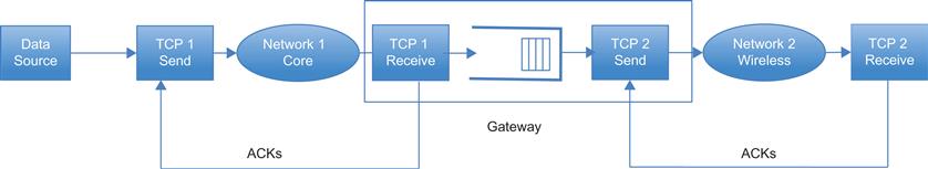
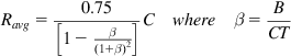
Hence, the change in window size is given by W(Ts−T)/Ts. This equation shows that Westwood uses a multiplicative decrease policy, where the amount of decrease is proportional to the queuing delay in the network. It follows that TCP Westwood falls in the class of additive increase/multiplicative decrease (AIMD) algorithms; however, the amount of decrease may be more or less than that of TCP Reno, depending on the congestion state of the network. Hence, it is important to investigate its fairness when competing with other Westwood connections and with Reno connections. Casetti et al. [4] carried out one such simulation study in which they showed that when competing with Reno connections, Westwood gets 16% more bandwidth than its fair share, which they deemed to be acceptable. Figure 4.3 shows the throughput of Westwood and Reno as a function of link error rate for a link of capacity 2 mbps. As can be seen, there is a big improvement in Westwood throughput over that of Reno when the loss rates are around 0.1%.
Other schemes to estimate the connection bandwidth include the work by Capone et al. [8] as part of their TCP TIBET algorithm, in which they use a modified version of the filter used in the Core Stateless Fair Queuing Estimation algorithm [9] and obtained good results. Another filter was proposed by Xu et al. [10] as part of their TCP Jersey design. This filter was derived from the Time Sliding Window (TSW) estimator that was proposed by Clarke and Fang [11].
4.4.1.1 TCP Westwood Throughput Analysis
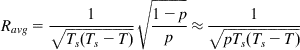
It has been shown by Greico and Mascolo [12] that the expected throughput of TCP Westwood in the presence of link error rate p is given by
(8)
Equation 8 can be derived used the machinery developed in Section 3.2.1 of Chapter 3, and we proceed to so next using the same notation that was used there. Recall that in the fluid limit, the window size for TCP Reno obeyed the following equation (equation 29 in Chapter 3):
(9)
For TCP Westwood, the first term on the RHS remains the same because this governs the window size increase during the congestion avoidance phase. The second term changes because the window decrease rule is different, and the resulting equation is given by
(10)
In equation 10 we replaced ![]() , which is window decrease rule for Reno by
, which is window decrease rule for Reno by ![]() , which the window change under Westwood. Next using the approximation that
, which the window change under Westwood. Next using the approximation that ![]() and
and ![]() , we obtain
, we obtain
(11)
Setting ![]() and Q(t)=P(t-T)=p, in equilibrium, we obtain
and Q(t)=P(t-T)=p, in equilibrium, we obtain
(12)
 (12)
(12)
where Ravg and p are the steady state values of R(t) and P(t), respectively.
Assuming that the queuing delay (Ts–T) can be written as a fraction k of the average round trip latency,
Then equation 12 can be written as

On comparing this equation with that for TCP Reno, it follows that TCP Westwood has the effect of a net reduction in link error rate by the fraction k. This reduction is greatest when the queuing delay is small compared with the end-to-end latency. From this, it follows that Westwood is most effective over long-distance links and least effective in local area network (LAN) environments with a lot of buffering.
4.4.2 Loss Discrimination Algorithm (LDA)
Loss Discrimination Algorithms are useful tools that can be used to differentiate between packet losses caused by congestion versus those caused by link errors. This information can be used at sender to appropriately react on receiving duplicate ACKs by not reducing the window size if link errors are the cause of the packet drop.
We will describe an LDA that was proposed by Fu and Liew as part of their TCP Veno algorithm [13]. This mechanism was inspired by the rules used by TCP Vegas to detect an increase in queue size along the connection’s path.
Readers may recall from the description of TCP Vegas from Chapter 1 that this algorithm uses the difference between expected throughput and the actual throughput values to gauge the amount of congestion in the network. Defining RE(t) to be the expected value of the throughput and D(t) the difference between the throughputs, we have
(13)
In equation 13, Ts is a smoothed value of the measured round trip time. By Little’s law, D(t) equals the queue backlog along the path.
The congestion indicator in the LDA is set to 0 if D(t) is less than 3 and is set to 1 otherwise. Fu and Liew [13] used this rule in conjunction with Reno’s regular multiplicative decrease rule and a slightly modified additive increase rule and observed a big increase in TCP performance in the presence of random errors.
Another LDA was proposed by Xu et al. [10] and works as follows: Unlike the LDA described earlier, this LDA requires that the network nodes pass on congestion information back to the source by appropriately marking the ACK packets traveling in the reverse direction if they observe that their average queue length has exceeded some threshold. The average queue length is computed using a low-pass filter in exactly the same way as for marking packets in the RED algorithm. The only difference is that a much more aggressive value for the smoothing parameter is used. Xu et al. [10] suggest a value of 0.2 for the smoothing parameter as opposed to 0.002, which is used for RED. Using this LDA, they showed that their algorithm, TCP Jersey, outperformed TCP Westwood for the case when the link error rate equaled or exceeded 1%, and they attributed this improvement to the additional boost provided by the LDA.
4.4.3 Zero Receive Window (ZRW) ACKs
A problem that is unique to wireless is that the link may get disconnected for extended periods, for a number of different reasons. When this happens, the TCP source will time out, perhaps more than once, resulting in a very large total time-out interval. As a result, even after the link comes back up, the source may still be in its time-out interval.
The situation described can be avoided by putting the TCP source into a state where it freezes all retransmit timers, does not cut down its congestion window size, and enters a persist mode. This is done by sending it an ACK in which the receive window size is set to zero. In this mode, the source starts sending periodic packets called Zero Window Probes (ZWPs). It continues to send these packets until the receiver responds to a ZWP with a nonzero window size, which restarts the transmission.
There have been two proposals in the literature that use ZRW ACKs to combat link disconnects:
• The Mobile TCP or M-TCP protocol by Brown and Singh [14]: M-TCP falls within the category of split-TCP designs, with the connection from the fixed host terminated at the gateway and a second TCP connection between the gateway and the client. However, unlike I-TCP, the gateway does not ACK a packet from the fixed host immediately on reception but waits until the packet has been ACK’d by the client, so that the system maintains end-to-end TCP semantics. In this design, the gateway node is responsible for detecting whether the mobile client is in the disconnect state by monitoring the ACKs flowing back from it on the second TCP connection. When the ACKs stop coming, the gateway node sends a zero window ACK back to the source node, which puts it in the persist mode. When the client gets connected again, the gateway sends it a regular ACK with a nonzero receive window in response to a ZWP to get the packets flowing again. To avoid the case in which the source transmits a window full of packets, all of which get lost over the second connection, so that there is no ACK stream coming back that can be used for the zero window ACK, Brown and Singh suggested that the gateway modify the ACKs being sent to the fixed host, so that the last byte is left un-ACKed. Hence, when the client disconnect does happen, the gateway can then send an ACK back to the fixed host with zero window indication.
• The Freeze TCP protocol by Goff et al. [15]: In this design, the zero window ACK is sent by the mobile client rather than the gateway. The authors made this choice for a couple of reasons, including (1) the mobile client has the best information about the start of a network disconnect (e.g., by detecting the start of a hand-off) and hence is a natural candidate to send the zero window ACK, and (2) they wanted to avoid any design impact on any node in the interior of the network so that Freeze TCP would work on an end-to-end basis. They also borrowed a feature from an earlier design by Cacares and Iftode [16] by which when the disconnect period ends, the client sends three Duplicate ACKs for the last data segment it received before the disconnection for the source to retransmit that packet and get the data flowing again. Note that Freeze TCP can be implemented in the context of the split-TCP architecture, such that the zero window ACKs can be sent by the mobile client to the gateway node to freeze the second TCP connection over the access network.
In general, client disconnect times have been steadily reducing as the mobile hand-off protocols improve from GPRS onward to LTE today. Hence, the author is not aware of any significant deployment of these types of protocols. They may be more relevant to wireless local area networks (WLANs) or ad-hoc networks in which obstructions could be the cause of link disconnects.
4.4.4 TCP with Available Bandwidth Estimates and Loss Discrimination Algorithms
The following pseudocode, adapted from Xu et al. [10], describes the modified congestion control algorithm in the presence of both the ABE and LDA algorithms. Note that the variable LDA is set to 1 if the sender decides that the packet loss is attributable to congestion and set to 0 if it is attributable to link errors. Also, SS, CA, fast_recovery, and explicit_retransmit are the usual TCP Reno Slow Start, Congestion Avoidance, Fast Recovery, and packet retransmission procedures as described in Chapter 1. An example of a rate_control procedure is the one given for TCP Westwood in Section 4.4.1.
recv( ) 1
{
ABE( ) 2
If ACK and LDA= 0 3
SS( ) or CA( ) 4
end if 5
if ACK and LDA= 1 6
rate_control( ) 7
SS( ) or CA( ) 8
end if 9
if nDUPACK and LDA = 1 10
rate control( ) 11
explicit_retransmit( ) 12
fast_recovery( ) 13
end if 14
if nDUPACK and LDA = 0 15
explicit_retransmit( ) 16
fast_recovery( ) 17
end if 18
}
Note that if packet loss is detected (nDUPACK=true) but LDA=0 (i.e., there is no congestion detected), then the source simply retransmits the missing packet (line 16) without invoking the rate_control procedure. On the other hand, even if there is no packet loss but congestion is detected, then the source invokes rate_control without doing any retransmits (lines 6–9).
4.5 Link-Level Error Correction and Recovery
A more direct way of solving the problem of link layer reliability is by reducing the effective error rate that is experienced by TCP. There are several ways this can be done:
• The problem can be attacked at the physical layer by using more powerful error-correcting codes. For example, LTE uses a sophisticated error correction scheme called Turbo Coding to accomplish this. Other error correction schemes in use include Reed-Solomon and convolutional coding [17].
• Link layer retransmissions or ARQ: As the name implies, the system tries to hide packet loss at the link layer by retransmitting them locally. This is a very popular (and effective) method, widely used in modern protocols such as LTE and WiMAX.
• Hybrid schemes: Both physical layer error correction and link layer retransmissions can be combined together in an algorithm known as Hybrid ARQ (HARQ). In these systems, when a packet arrives in error at the receiver, instead of discarding it, the receiver combines its signal with that of the subsequent retransmission, thereby obtaining a stronger signal at the physical layer. Modern wireless systems such as LTE and WiMAX have deployed HARQ.
From theoretical studies as well as practical experience from deployed wireless networks, link layer techniques have proven very effective in combating link errors. As a result, all deployed cellular data networks, including 3G, LTE, and WiMAX, include powerful ARQ and FEC components at the wireless link layer.
4.5.1 Performance of TCP with Link-Level Forward Error Correction (FEC)
Link-level FEC techniques include algorithms such as convolutional coding, turbo coding, and Reed-Solomon coding, and all modern cellular protocols, including 3G and LTE, incorporate them as part of the physical layer. FEC algorithms were discovered in the 1950s, but until 1980 or so, their use was confined to space and military communications because of the large processing power they required. With the advances in semiconductor technology, link-level FEC is now incorporated in every wireless communication protocol today and has started to move up the stack to the transport and even application layers. The algorithms have also become better with time; for example, turbo coding, which was discovered in the 1990s, is a very powerful algorithm that takes the system close to the theoretical Shannon bound. When compared with ARQ, FEC has some advantages; ARQ results in additional variable latency because of retransmissions that can throw off the TCP retransmit timer, but this is not an issue for FEC. This is especially problematic for long satellite links, for which ARQ may be an inappropriate solution.
Following Barakat and Altman [18], we present an analysis of the TCP throughput over a link that is using a link-level block FEC scheme such as Reed-Solomon coding.
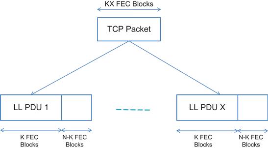
Define the following (Figure 4.4):
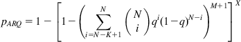
X: Number of link-level transmission units (called LL PDUs) formed from a single TCP packet
T: Minimum round trip latency for TCP
q: Probability that a LL PDU is received in error in the absence of FEC
qT: Probability that a LL PDU is received in error in the presence of FEC
(N,K): Parameters of the FEC scheme, which uses a block code [17]. This consists of K FEC units of data, to which the codec adds (N-K) FEC units of redundant coding data, such that each LL PDU consists of N units in total.
pFEC(N,K): Probability that a TCP packet is lost in the presence of FEC with parameters (N,K)
We now use the square-root formula (see Chapter 2) to derive an expression for the TCP throughput as a function of the link and FEC parameters.
Because there are KX FEC data units that make up a TCP packet, it follows that the average TCP throughput in the presence of FEC with parameters (N,K) is given by
(14)
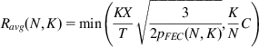 (14)
(14)
Also, as a result of the block FEC, the link capacity reduces by a factor of (K/N).
We now derive an expression for the TCP packet loss probability p(N,K).
A TCP packet is lost when one or more of the X LL PDUs that constitute it arrive in error. Hence, it follows that
(15)
An LL PDU is lost when more than (N-K) of its FEC block units are lost because of transmission errors, which happens with probability
(16)
From equations 15 and 16, it follows that the probability that a TCP packet is lost is given by
(17)
 (17)
(17)
From equation 16, it is clear that the addition of FEC reduces the loss probability of LL PDUs (and as a result that of TCP packets), which results in an increase in TCP throughput as long as the first term in the minimum in equation 14 is less than the second term. As we increase N, we reach a point where the two terms become equal, and at this point, the FEC entirely eliminates all link errors. Any increase in FEC beyond this point results in the deterioration of TCP throughput (i.e., there is more FEC than needed to clean up the link). This implies that the optimal amount of FEC is the one that causes the two terms in equation 14 to be equal, that is,
(18)
 (18)
(18)
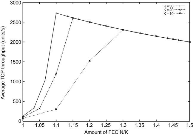
Figure 4.5 plots the TCP throughput as a function of the ratio N/K, for K=10, 20, and 30. Increasing N/K while keeping K fixed leads to more FEC blocks per LL PDU, which increases the resulting throughput. Figure 4.5 also plots (K/N)C and the intersection of this curve with the throughput curve is the point that is predicted by equation 18 with the optimal amount of FEC.
The analysis presented assumed that the LL PDU loss probabilities form an iid process. A more realistic model is to assume the Gilbert loss model, in which errors occur in bursts. This reflects the physics of an actual wireless channel in which burst errors are common because of link fading conditions. However, this complicates the analysis considerably, and a closed form simple expression is no longer achievable. Interested readers are referred to Barakat and Altman [18] for details of the analysis of this more complex model.
4.5.2 Performance of TCP with Link-Level Automatic Retransmissions and Forward Error Correction
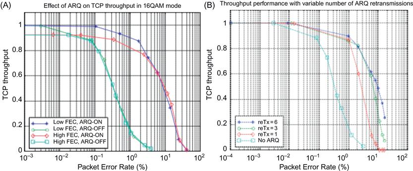
Link-level ARQ or retransmission is an extremely effective way of reducing the link error rate. Figures 4.6A and 4.6B are plotted from measurements made from a functioning broadband wireless system [19] that has been commercially deployed. As shown in Figure 4.6A, even with an error rate as high as 10%, the TCP throughput remains at 40% of the maximum. Figure 4.6B shows that the throughput performance improves as the number of ARQ retransmissions is increased, but after six or so retransmissions, there is no further improvement. This is because at high error rates, the number of retransmissions required to recover a packet grows so large that the resulting increase in end-to-end latency causes the TCP retransmit timer to expire, thus resulting in a time-out. This observation also points to an important issue when using ARQ at the link layer. Because of its interaction with TCP’s retransmissions, ARQ can in fact make the overall performance worse if not used carefully. Hence, some guidelines for its use include:
• The maximum number of ARQ retransmissions should be capable of being configured to a finite number, and if the LL-PDU is still received in error, then it should be discarded (and let TCP recover the packet). The max number of retransmissions should be set such the total time to do so is significantly less than the TCP retransmit time-out (RTO) interval.
• ARQ should be configurable on a per connection basis, so that connections that do not need the extra reliability can either turn it off or reduce the number of retransmissions.
Modern implementations of ARQ in wireless protocols such as LTE or WiMAX follow these rules in their design.
In this section, following Barakat and Fawal [20], we extend the analysis in Section 4.5.1 to analyze the performance of TCP over a link implementing a Selective Repeat ARQ scheme (in addition to FEC) and in-order delivery of packets to the IP layer at the receiver. We will reuse the definitions used in Section 4.5.1, so that a TCP packet of size KX FEC blocks is split into X LL PDUs, each of which is made up of K FEC blocks (see Figure 4.4). To each of these K FEC blocks we add (N-K) redundant FEC blocks to obtain a Reed Solomon–encoded LL PDU of size N FEC blocks. If the FEC does not succeed in decoding an LL PDU, the SR-ARQ scheme is invoked to recover it by doing retransmissions. The retransmissions will be done a maximum number of times, denoted by M. If the LL PDU fails to get through even after M retransmissions, the ARQ-SR assumes that it cannot be recovered and leaves its recovery to TCP.
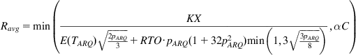
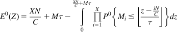
Recall from equation 52 in Chapter 2 that the expression for average TCP throughput in the presence of random loss and time-outs is given by
(19)
 (19)
(19)
where the throughput is in units of FEC units per second and ![]() is the fraction of the link bandwidth lost because of the FEC and LL PDU retransmissions, pARQ is the probability that a TCP packet is lost despite ARQ, E(TARQ) is the average round trip latency, C is the capacity of the link, and RTO is the TCP timeout value.
is the fraction of the link bandwidth lost because of the FEC and LL PDU retransmissions, pARQ is the probability that a TCP packet is lost despite ARQ, E(TARQ) is the average round trip latency, C is the capacity of the link, and RTO is the TCP timeout value.
Note that in equation 19, we have replaced T, which is the nonqueuing part of the round trip latency in equation 52 of Chapter 2, by the average value E(TARQ). The reason for this is that in the presence of ARQ, the nonqueuing part of the round trip latency is no longer fixed but varies randomly depending on the number of link retransmissions.
As in the previous section, we will assume that q is the probability that an LL PDU transmission fails because of link errors in the absence of FEC and ARQ. Note that to find Ravg, we need to find expressions for E(TARQ), pARQ, and ![]() as functions of the link, ARQ, and FEC parameters q, N, K, M, and X.
as functions of the link, ARQ, and FEC parameters q, N, K, M, and X.
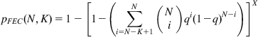
The ARQ-SR receiver acknowledges each LL PDU either with an ACK or a NACK. The LL PDUs that are correctly received are resequenced before being passed on to the IP layer. A TCP packet is lost if one or more of its constituent LL PDUs is lost. Under the assumption that LL PDUs are lost independently of each other with loss rate qF, we obtain the probability of a TCP packet loss as
(20)
We now obtain an expression for qF. Note that an LL PDU is lost if all M retransmissions fail, in addition to the loss of the original transmission, for a total of (M+1) tries. The probability that a single LL PDU transmission fails in the absence of ARQ but with FEC included is given by
(21)
so that the probability that an LL PDU is lost after the M ARQ retransmissions is given by
(22)
By substituting equation 22 in equation 20, we obtain the following expression for the TCP packet loss probability pARQ in the presence of both FEC and ARQ:
(23)
 (23)
(23)
To obtain an expression for ![]() , which is the amount of link bandwidth left over after the FEC and ARQ overheads are accounted for, note the following:
, which is the amount of link bandwidth left over after the FEC and ARQ overheads are accounted for, note the following:
• A fraction (K/N) of the link bandwidth is lost because of the FEC overhead.
• A fraction (1−qT) of the link bandwidth is lost because of dropping of LL PDUs that arrive in error.
• A fraction (1−qF)X−1 of the link bandwidth is lost because of LL PDUs that arrive intact but are dropped anyway because one or more of the other (X−1) LL PDUs that are part of the same TCP packet do not arrive intact, despite the M retransmissions.
Hence, the fraction of the link bandwidth that is available for TCP packet transmission is given by
(24)
We next turn to the task of finding the average round trip latency E(TARQ) for the TCP packets.
![]() : The time interval from the start of transmission of an LL PDU and the receipt of its acknowledgement
: The time interval from the start of transmission of an LL PDU and the receipt of its acknowledgement
D: One-way propagation delay across the link
Mi: Number of retransmissions for the ith packet, ![]() , until it is delivered error free. Note that
, until it is delivered error free. Note that ![]() .
.
T0: Average round trip latency for the TCP packet, excluding the delay across the bottleneck link
t, t0: Random variables whose average equals T and T0, respectively
Then ![]() is given by
is given by
(25)
Assume that all the X LL PDUs that make up a TCP packet are transmitted back to back across the link. Then the ith LL PDU starts transmission at time ![]() , and it takes
, and it takes ![]() seconds to finish its transmission and receive a positive acknowledgement. Hence, it follows that
seconds to finish its transmission and receive a positive acknowledgement. Hence, it follows that
(26)
We will now compute the expected value of t under the condition that the TCP packet whose delay is being computed has been able to finish its transmission.
Define Z as
(27)
It follows that
(28)
where
(29)
Note that the upper limit of integration is given by ![]() because this is the maximum value of Z. Note that
because this is the maximum value of Z. Note that
(30)
so that
(31)
 (31)
(31)
Next we derive a formula for the probability distribution for Mi.
Note that the probability that all X LL PDUs that make up the packet are received successfully (after ARQ) is given by ![]() because the
because the ![]() is the probability that an LL PDU is received in error even after M retransmissions. It follows that
is the probability that an LL PDU is received in error even after M retransmissions. It follows that
(32)
 (32)
(32)
Equations 23 and 32 can then be used to evaluate E0(Z) in equation 31. This allows us to evaluate T in equation 28 and subsequently the average TCP throughput by using equation 19.
4.6 The Bufferbloat Problem in Cellular Wireless Systems
Until this point in this chapter, we have focused on the random packet errors as the main cause of performance degradation in wireless links. With advances in channel coding and smart antenna technology, as well as powerful ARQ techniques such as HARQ, this problem has been largely solved in recently designed protocols such as LTE. However, packet losses have been replaced by another link related problem, which is the large variability in wireless link latency. This can also lead to a significant degradation in system performance as explained below.
Recall from Chapter 2 that for the case when there are enough buffers to accommodate the maximum window size Wmax, the steady-state maximum buffer occupancy at the bottleneck link is given by:
(33)
From this we concluded that if the maximum window size is kept near CT, then the steady state buffer occupancy will be close to zero, which is the ideal operating case. In reaching this conclusion, we made the critical assumption that C is fixed, which is not the case for the wireless link. If C varies with time, then one of the following will happen:
• If C>Wmax/T, then bmax=0, i that is, there is no queue build at the bottleneck, and in fact the link is underused
• If C<<Wmax/T, then a large steady-state queue backlog will develop at the bottleneck, which will result in an increase in the round trip latency if the buffer size B is large. This phenomenon is known as bufferbloat.
Note that buffer size B at the wireless base station is usually kept large to account for the time needed to do ARQ and to keep a reservoir of bits ready in case the capacity of the link suddenly increases. Because C is constantly varying, the buffer will switch from the empty to the full state frequently, and when it is in the full state, it will cause a degradation in the performance of all the interactive applications that are using that link. Queuing delays of the order of several seconds have been measured on cellular links because of this, which is unacceptable for applications such as Skype, Google Hangouts, and so on. Also, the presence of a large steady-state queue size means that transient packet bursts, such as those generated in the slow-start phase of a TCP session, will not find enough buffers, which will result in multiple packet drops, leading to throughput degradation.
There are two main causes for the variation in link capacity:
• ARQ related retransmissions: If the ARQ parameters are not set properly, then the retransmissions can cause the link latency to go up and the capacity to go down.
• Link capacity variations caused by wireless link adaptation: This is the more important cause of capacity changes and is unique to wireless links. To maintain the robustness of transmissions, the wireless base station constantly monitors the quality of the link to each mobile separately, and if it detects problems, then it tries to make the link more robust by changing the modulation, coding or both. For instance, in LTE, the modulation can vary from a high of 256-QAM to a low of QPSK, and in the latter case, the link capacity is less than 25% of the former. This link adaptation is done on a user-by-user basis so that any point in time different mobiles get different performance depending on their link condition. The base station implements this system, by giving each mobile its own buffer space and a fixed time slot for transmission, and it serves the mobiles on a round robin basis. Depending on the current modulation and coding, different mobiles transmit different amounts of data in their slot, which results in the varying link capacity (Figure 4.7). In Figure 4.7 mobile 1 has the best link, so it uses the best modulation, which enables it to fit 100 bytes in its slot; mobile 2 has the worst link and the lowest modulation, so it can fit only 50 bytes in its slot.
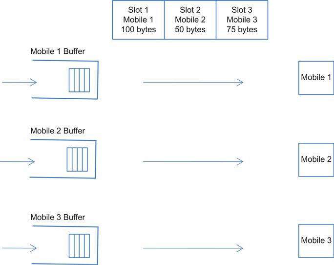
From the description of the link scheduling that was given earlier, it follows that the traffic belonging to different mobiles does not get multiplexed together at the base station (i.e., as shown in Figure 4.7, a buffer only contains traffic going to single mobile). Hence, the congestion that a connection experiences is “self-inflicted” and not attributable to the congestive state of other connections.
Note that the rule of thumb that is used in wireline links to size up the buffer size (i.e., B=CT) does not work any longer because the optimal size is constantly varying with the link capacity. The bufferbloat problem also cannot be solved by simply reducing the size of the buffer because this will cause problems with the other functions that a base station has to carry out, such as reserving buffer space for retransmissions or deep packet inspections.
Solving for bufferbloat is a very active research topic, and the networking community has not settled on a solution yet, but the two areas that are being actively investigated are Active Queue Management (AQM) algorithms (see Section 4.6.1) and the use of congestion control protocols that are controlled by end-to-end delay (see Section 4.6.2).
4.6.1 Active Queue Management (AQM) Techniques to Combat Bufferbloat
AQM techniques such as Random Early Detection (RED) were designed in the mid 1990s but have not seen widespread deployment because of the difficulty in configuring them with the appropriate parameters. Also, the steadily increasing link speeds in wireline networks kept the network queues under control, so operators did not feel the need for AQM. However, the bufferbloat problem in cellular networks confronted them with a situation in which the size of the bottleneck queue became a serious hindrance to the system performance; hence, several researchers have revisited the use of traditional RED in controlling the queue size; this work is covered in Section 4.6.1.1.
Nichols and Jacobsen [21] have recently come up with a new AQM scheme called Controlled Delay (CoDel) that does not involve any parameter tuning and hence is easier to deploy. It is based on using delay in the bottleneck buffer, rather than its queue size, as the indicator for link congestion. This work is covered in Section 4.6.1.2.
4.6.1.1 Adaptive Random Early Detection
Recall from the description of RED in Chapter 1, that the algorithm requires that the operators choose the following parameters: the queue thresholds minth and maxth, the maximum dropping probability maxp and the averaging parameter wq. If the parameters are not set properly, then the analysis in Chapter 3 showed that it can lead to queue length oscillations, low link utilizations, or buffer saturation, resulting in excessive packet loss. Using the formulae in Chapter 3, it is possible to choose the appropriate parameters for a given value of the link capacity C, the number of connections N, and the round trip latency T. However, if any of these parameters is varying, as C is in the wireless case, then the optimal parameters will also have to change to keep up with it (i.e., they have to become adaptive).
Adaptive RED (ARED) was designed to solve the problem of automatically setting RED’s parameters [22]. It uses the “gentle” version of RED, as shown in Figure 4.8. The operator has to set a single parameter, which is the target queue size, and all the other parameters are automatically set and adjusted over time, as a function of this. The main idea behind the adaptation in ARED is the following: With reference to Figure 4.8, assuming that averaging parameter wq and the thresholds minth and maxth are fixed, the packet drop probability increases if the parameter maxp is increased and conversely decreases when maxp is reduced. Hence, ARED can keep the buffer occupancy around a target level by increasing maxp if the buffer size is more than the target and decreasing maxp if the buffer size falls below the target. This idea was originally proposed by Feng et al. [23] and later improved upon by Floyd et al. [22], who used an AIMD approach to varying maxp, as opposed to multiplicative increase/multiplicative decrease (MIMD) algorithm used by Feng et al. [23]
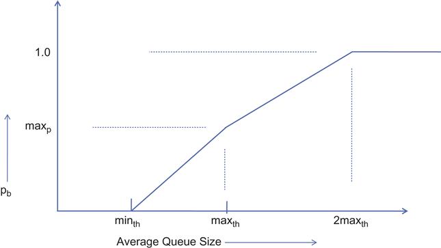
The ARED algorithm is as follows:
ared( )
Every interval seconds:
If (avg> target and maxp <= 0.5)
Increase maxp:
maxp ← maxp + a
elseif (avg<target and maxp>= 0.01)
Decrease maxp:
maxp ← maxp * b 1
The parameters in this algorithm are set as follows:
Avg: The smoothed average of the queue size computes as
(34)
interval: The algorithm is run periodically every interval seconds, where interval=0.5 sec
a: The additive increment factor is set to a=min(0.01, maxp/4).
b: The multiplicative decrement factor is set to 0.9.
target: The target for the average queue size is set to the interval
minth: This is the only parameter that needs to be manually set by the operator.
ARED was originally designed for wireline links, in which the capacity C is fixed and the variability is attributable to the changing load on the link (i.e., the number of TCP connections N). The algorithm needs to be adapted for the wireless case, in particular the use of equation 34 to choose wq needs to be clarified because C is now varying. If wq is chosen to be too large relative to the link speed, then it causes queue oscillations because the average tends to follow the instantaneous variations in queue size. Hence, one option is to choose the maximum possible value for the link capacity in equation 34, which would correspond to the mobile occupying the entire channel at the maximum modulation.
Also, the value of interval needs to be revisited because the time intervals during which the capacity changes are likely to be different than the time intervals during which the load on the link changes. Floyd et al. [22] showed through simulations that with interval=0.5 sec, it takes about 10 sec for ARED to react to an increase in load and bring the queue size back to the target level. This is likely too long for a wireless channel, so a smaller value of interval is more appropriate.
4.6.1.2 Controlled Delay (CoDel) Active Queue Management
The CoDel algorithm is based on the following observations about bufferbloat, which were made by Nichols and Jacobsen [21]:
• Networks buffers exist to absorb transient packet bursts, such as those that are generated during the slow-start phase of TCP Reno. The queues generated by these bursts typically disperse after a time period equal to the round trip latency of the system. They called this the “good” queue. In a wireless system, queue spikes can also be caused to temporary decreases in the link capacity.
• Queues that are generated because of a mismatch between the window size and the delay bandwidth product, as given by equation 33, are “bad” queues because they are persistent or long term in nature and add to the delay without increasing the throughput. These queues are the main source of bufferbloat, and a solution is needed for them.
Based on these observations, they gave their CoDel algorithm the following properties:
• Similar to the ARED algorithm, it is parameter-less
• It treats the “good” queue and “bad” queues, differently, that is, it allows transient bursts to pass through while keeping the nontransient queue under control.
• Unlike RED, it is insensitive to round trip latency, link rates, and traffic loads.
• It adapts to changing link rates while keeping utilization high.
The main innovation in CoDel is to use the packet sojourn time as the congestion indicator rather than the queue size. This comes with the following benefits: Unlike the queue length, the sojourn time scales naturally with the link capacity. Hence, whereas a larger queue size is acceptable if the link rate is high, it can become a problem when the link rate decreases. This change is captured by the sojourn time. Hence, the sojourn time reflects the actual congestion experienced by a packet, independent of the link capacity.
CoDel tracks the minimum sojourn time experienced by a packet, rather than the average sojourn time, because the average can be high even for the “good” queue case (e.g., if a maximum queue size of N disperses after one round trip time, the average is still N/2). On the other hand, if there is even one packet that has zero sojourn time, then it indicates the absence of a persistent queue. The minimum sojourn time is tracked over an interval equal to the maximum round trip latency over all connections using the link. Moreover, because the sojourn time can only decrease when a packet is dequeued, CoDel only needs to be invoked at packet dequeue time.
To compute an appropriate value for the target minimum sojourn time, consider the following equation for the average throughput that was derived in Section 2.2.2 of Chapter 2:
(35)
 (35)
(35)
Even at ![]() , equation 37 gives
, equation 37 gives ![]() . Because
. Because ![]() can be also interpreted as
can be also interpreted as ![]() =(Persistent sojourn time)/T, it follows that the above choice can also be interpreted as: The persistent sojourn time threshold should be set to 5% of the round trip latency, and this is what Nichols and Jacobsen recommend. The sojourn time is measured by time stamping every packet that arrives into the queue and then noting the time when it leaves the queue.
=(Persistent sojourn time)/T, it follows that the above choice can also be interpreted as: The persistent sojourn time threshold should be set to 5% of the round trip latency, and this is what Nichols and Jacobsen recommend. The sojourn time is measured by time stamping every packet that arrives into the queue and then noting the time when it leaves the queue.
When the minimum sojourn time exceeds the target value for at least one round trip interval, a packet is dropped from the tail of the queue. The next dropping interval is decreased in inverse proportion to the square root to the number of drops since the dropping state was entered. As per the analysis in Chapter 2, this leads to a gradual linear decrease in the TCP throughput, as can be seen as follows: Let N(n) and T(n) be the number of packets transmitted in nth drop interval and the duration of the nth drop interval, respectively. Then the TCP throughput R(n) during the nth drop interval is given by
(36)
Note that ![]() , while N(n) is given by the formula (see Section 2.3, Chapter 2)
, while N(n) is given by the formula (see Section 2.3, Chapter 2)
(37)
where Wm(n) is the maximum window size achieved during the nth drop interval. Because the increase in window size during each drop interval is proportional to the size of the interval, it follows that ![]() , from which it follows from equation 37 that
, from which it follows from equation 37 that ![]() . Plugging these into equation 36, we finally obtain that
. Plugging these into equation 36, we finally obtain that ![]() .
.
The throughput decreases with n until the minimum sojourn time falls below the threshold at which time the controller leaves the dropping state. In addition, no drops are carried out if the queue contains less than one packet worth of bytes.
One way of understanding the way CoDel works is with the help of a performance measure called Power, defined by
Algorithms such as Reno and CUBIC try to maximize the throughput without paying any attention to the delay component. As a result, we see that in variable capacity links, the delay blows up because of the large queues that result. AQM algorithms such as RED (and its variants such as ARED) and CoDel, on the other hand, can be used to maximize the Power instead by trading off some of the throughput for a lower delay. On an LTE link, simulations have shown that Reno achieves almost two times the throughput when CoDel is not used; hence, the tradeoff is quite evident here. The reasons for the lower throughputs with CoDel are the following:
• As shown using equation 35, even without a variable link capacity, the delay threshold in CoDel is chosen such that the resulting average throughput is about 78% of the link capacity.
• In a variable capacity link, when the capacity increases, it is better to have a large backlog (i.e., bufferbloat) because the system can keep the link fully utilized. With a scheme such as CoDel, on the other hand, the buffer soon empties in this scenario, and as a result, some of the throughput is lost.
Hence, CoDel is most effective when the application needs both high throughput as well as low latency (e.g., video conferencing) or when lower speed interactive applications such as web surfing are mixed with bulk file transfers in the same buffer. In the latter case, CoDel considerably improves the latency of the interactive application at the cost of a decrease in the throughput of the bulk transfer application. If Fair Queuing is combined with CoDel, so that each application is given its own buffer, then this mixing of traffic does not happen, in which CoDel can solely be used to improve the performance of applications of the video conferencing type.
The analysis presented above also points to the fact that the most appropriate buffer management scheme to use is a function of the application. This idea is explored more fully in Chapter 9.
4.6.2 End-to-End Approaches Against Bufferbloat
AQM techniques against bufferbloat can be deployed only if the designer has access to the wireless base station whose buffer management policy is amenable to being changed. If this is not the case, then one can use congestion control schemes that work on an end-to-end basis but are also capable of controlling delay along their path. If it is not feasible to change the congestion algorithm in the remote-end server, then the split-TCP architecture from Section 4.3 can be used (see Figure 4.2). In this case, the new algorithm can be deployed on the gateway (or some other box along the path) while the legacy TCP stack continues to run from the server to the gateway.
In this section, we will describe a congestion control algorithms called Low Extra Delay Background Transport (LEDBAT) that is able to regulate the connections’ end-to-end latency to some target value. We have already come across another algorithm that belongs to this category (i.e., TCP Vegas; see Chapter 1).
In general, protocols that use queuing delay (or queue size) as their congestion indicator, have an intrinsic disadvantage when competing with protocols such as Reno that use packet drops as the congestion indicator. The former tends to back off as soon as the queues start to build up, allowing the latter to occupy the all the bandwidth. However, if the system is designed in the split-connection approach, then the operator has the option of excluding the Reno-type algorithm entirely from the wireless subnetwork, so the unfairness issue will not arise in practice.
4.6.2.1 TCP LEDBAT
LEDBAT has been Bit Torrent’s default transport protocol since 2010 [24] and as a result now accounts for a significant share of the total traffic on the Internet. LEDBAT belongs to the class of Less than Best Effort (LBE) protocols, which are designed for transporting background data. The design objective of these protocols is to grab as much of the unused bandwidth on a link as possible, and if the link starts to get congested, then quickly back off.
Even though LEDBAT was designed to be a LBE protocol, its properties make it suitable to be used in wireless networks suffering from bufferbloat. This is because LEDBAT constantly monitors its one-way link latency, and if it exceeds a configurable threshold, then it backs off its congestion window. As a result, if the wireless link capacity suddenly decreases, then LEDBAT will quickly detect the resulting increase in latency caused by the backlog that is created and decrease its sending rate. Note that if the split-TCP design is used, then only LEDBAT flow will be present at the base station (and furthermore, they will be isolated from each other), so that LEDBAT’s reduction in rate in the presence of regular TCP will never be invoked.
LEDBAT requires that that each packet carry a timestamp from the sender, which the receiver uses to compute the one-way delay from the sender, and sends this computed value back to the sender in the ACK packet. The use of the one-way delay avoids the complications that arise in other delay-based protocols such as TCP Vegas that use the round trip latency as the congestion signal, and as a result delays experienced by ACK packets in the reverse link introduce errors in the forward delay estimates.
![]() : Measured one-way delay between the sender and receiver
: Measured one-way delay between the sender and receiver
![]() : The maximum queuing delay that LEDBAT may itself introduce into the network, which is set to 100 ms or less
: The maximum queuing delay that LEDBAT may itself introduce into the network, which is set to 100 ms or less
T: Minimum measured one-way downlink delay
![]() : The gain value for the algorithm, which is set to one or less.
: The gain value for the algorithm, which is set to one or less.
The window increase–decrease rules for LEDBAT are as follows (per RTT):
(38)
if no loss and
(39)
on packet loss.
LEDBAT tries to maintain a fixed packet delay of ![]() seconds at the bottleneck. If the current queuing delay given by
seconds at the bottleneck. If the current queuing delay given by ![]() , exceeds the target
, exceeds the target ![]() , then the window is reduced in proportion to their ratio. When the measured queuing delay less that the target
, then the window is reduced in proportion to their ratio. When the measured queuing delay less that the target ![]() , then LEDBAT increases its window, but the amount of increase per RTT can never exceed 1.
, then LEDBAT increases its window, but the amount of increase per RTT can never exceed 1.
There are some interesting contrasts between LEDBAT and Westwood even though their designs are similar:
• Whereas Westwood uses a smoothed estimate of the round trip latency to measure congestion, LEDBAT uses the latest unfiltered 1-way latency.
• LEDBAT is less aggressive in its window increase rule because Westwood follows Reno in increasing its window by 1 every RTT, but LEDBAT uses a window increase that is less than 1.
• The rule that LEDBAT uses to decrease its window size in congestion is similar to the one that Westwood uses on encountering a packet loss, as seen below:
Hence, in both cases, the decrease is proportional to the amount of congestion delay, but in LEDBAT, the decrease is additive, but in Westwood, it is multiplicative.
Note that even though two different clocks are used to measure the one-way delays in LEDBAT because only the difference ![]() appears in equation 38, any errors attributable to a lack of synchronization get cancelled out.
appears in equation 38, any errors attributable to a lack of synchronization get cancelled out.
LEDBAT has been shown to have intraprotocol fairness issue if multiple LEDBAT connections are competing for bandwidth at a single node. If the bottleneck is at the wireless base station, then interaction between LEDBAT flows from different mobiles should not be an issue, since the per mobile queues are segregated from each other.
4.7 Some Design Rules
The following rules, which are based on the material in this chapter, can be used for designing congestion control systems that traverse wireless links:
• Compute the quantity p(CT)2 for the system where p is the packet drop rate. If this number is around 8/3, then most of the packet drops are to buffer overflows rather than link errors, so no extra steps are needed to bring down the link error rate (refer to the discussion in Section 2.3.2 of Chapter 2 for the justification for this rule).
• If p(CT)2>>8/3, then the packet drops are being caused predominantly because of link errors. Furthermore, the link error rate is too high, and additional steps need to be taken to bring it down.
• If the wireless link supports Reed-Solomon FEC, then use equation 20 to compute pFEC, which is the link error rate in the presence of FEC. If pFEC(CT)2~8/3, then FEC is sufficient for good performance.
• If pFEC(CT)2>>8/3, then FEC is not sufficient. If the wireless link supports ARQ, then use equation 25 to compute pARQ, which is the link error rate with both ARQ and FEC. If pARQ(CT)2~8/3 for a certain number of retransmissions M, then link-level ARQ+FEC is sufficient for good performance.
• If FEC or ARQ are not available on the wireless link or if they do not result in a sufficient reduction in the error rate, then use the Transport layer techniques from Sections 4.3 and 4.4.
– If the TCP stack at the source is under the designer’s control, then techniques such TCP Westwood with ABE, LDA, or ZRW can be implemented.
– If the TCP stack at the source is not under the designer’s control, then use a split-level TCP design, with the splitting point implemented at a gateway-type device. In this case, techniques such as Westwood, ABE, or LDA can be implemented on the TCP2 connection.
If the link error rate is zero but the link shows large capacity variations, then bufferbloat may occur, and the following steps should be taken to limit it:
• If the base station software can be modified, then AQM schemes such ARED or CoDel should be used.
• If AQM is not an option, then the delay-based TCP protocols such as LEDBAT or Vegas should be used. This should be done in conjunction with a split-connection TCP architecture so that regular TCP continues to be used in the core packet network.
4.8 Further Reading
The techniques discussed in this chapter to mitigate packet losses work at either the transport layer (e.g., Westwood) or at the link layer (e.g., FEC or ARQ). However, some algorithms work cross-layer; the most well known among these is an algorithm called Snoop [25,26]. Snoop can be implemented at an intermediate point along the session path, either at the gateway or the base station. It works as follows: Downlink packets from the source are intercepted by Snoop and stored until it detects an ACK for that packet from the client. If a packet is lost, then Snoop intercepts the duplicate ACKs and suppresses them. It then retransmits the missing packet from its local cache, so that the source does not become aware of the loss. Hence, in some sense, Snoop operates like a TCP-aware link-level ARQ protocol.
Wireless links sometimes exhibit a large increase in their end-to-end latency because of link-level ARQ retransmissions or because of the extra latency during handoffs. This causes the TCP retransmit timer to time out even though no packets were lost. When the ACK for the retransmitted packet arrives, the source is not able to tell whether this ACK was for the original transmission or for the retransmission (this is called the ACK ambiguity problem) and assumes the latter. This leads to the retransmission of the entire window of packets. To correct this problem, Ludwig and Katz [27] designed an algorithm called TCP Eifel, which solves the ACK ambiguity problem by time stamping every TCP data packet and then having the receiver time stamp returning ACKs with the time stamp of the packet being ACK’d.