and hence is stable. Note that the fact that PM>0 implies that ![]() , where
, where ![]() is the frequency at which
is the frequency at which ![]() , that is, the gain margin is also positive.
, that is, the gain margin is also positive.
From Equation 67 it follows that
Since
it follows that
so that ![]() radians. Equation 69 also implies that
radians. Equation 69 also implies that
which implies that the ![]() . This proves equation 72 and consequently the stability result.
. This proves equation 72 and consequently the stability result.
The following example from Holot et al. [6] shows how equations 68 and 69 can be used to obtain appropriate RED parameters:
Consider the case: C=3750 packets/sec, ![]() and
and ![]() . From equation 69, it follows that
. From equation 69, it follows that
Choosing K=0.005, it follows from equation 68 that ![]() . Choosing maxp=0.1 and because
. Choosing maxp=0.1 and because ![]() , it follows that
, it follows that ![]() packets. The other RED parameters are calculated as
packets. The other RED parameters are calculated as ![]() , which yields
, which yields ![]() .
.
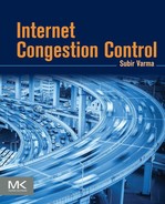
Figure 3.9A shows the case when the RED parameters are set without taking equation 68 into account, and we can observe the large buffer oscillations that result. When the parameters are set as per equation 68, then they result in a smoother buffer variation as shown in Figure 3.9B. Note the large amount of time that it takes for the queue to settle down in Figure 3.9B, which is a consequence of the small value of ![]() that was used to get a good phase margin.
that was used to get a good phase margin.
As the link capacity C or the round trip latency increases or the number N of connections decreases, the RED parameters Lred and K have to be changed to maintain the inequality (equation 68). We can do the following:
• Adapt Lred: This can be done by changing the value of the marking probability maxp while keeping the queue thresholds the same. Note that reducing maxp has the effect of reducing the number of dropped or marked packets when the average queue size is between the threshold values. This causes the queue size to increase beyond maxth, thus leading to increased packet drops because of buffer overflow. On the other hand, increasing maxp has the effect of increasing the number of RED drops and thus decreasing throughput. By using equation 68 as a guide, it is possible to adapt Lred more intelligently as a function of changing parameters. An alternative technique for adapting RED was given by Feng et al. [14], in which they used the behavior of the average queue size to adapt maxp. Thus, if the queue size spent most of its time near maxth, then maxp was increased, and if it spent most of its time at minth or under, maxp was reduced.
• Adapt K: From equation 64, K can be reduced by decreasing the averaging constant wq. However, note that decreasing wq causes the smoothing function to become less responsive to queue length fluctuations, which again leads to poorer regulation of the queue size.
From equation 69, as the round trip latency increases, ![]() decreases, which increases the time required for the queue to settle down. We can compensate by increasing the constant from 0.1, but the earlier analysis showed that this has the effect of decreasing the PM and thus increasing the queue oscillations.
decreases, which increases the time required for the queue to settle down. We can compensate by increasing the constant from 0.1, but the earlier analysis showed that this has the effect of decreasing the PM and thus increasing the queue oscillations.
3.4.1.2 Proportional Controllers
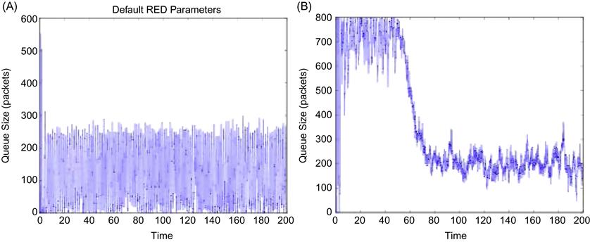
As shown in Figure 3.10, the RED controller from Figure 3.8 reduces to a proportional controller if K is chosen to be very large, which also corresponds to removing the low-pass filter entirely. This implies that the feedback from the bottleneck node is simply a scaled version of the (slightly delayed) queue length delta rather than the average queue length.
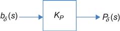
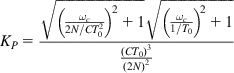
If we denote the proportionality factor by KP, then from equation 65, it follows that the transfer function is given by
 (74)
(74)
and in the frequency domain
We now carry out a stability analysis for this system using the same procedure that was used for the RED controller. Hence, we will choose a critical frequency ![]() such that with the appropriate choice of the controller parameters
such that with the appropriate choice of the controller parameters ![]() , and then show that the PM at
, and then show that the PM at ![]() is positive, which is sufficient to prove stability.
is positive, which is sufficient to prove stability.
If we choose ![]() as the geometric mean of the roots
as the geometric mean of the roots ![]() and
and ![]() so that
so that
 (75)
(75)
then under the condition
 (76)
(76)
it follows from equation 74 that ![]() . Note that this choice of Kp precisely cancels out the high loop gain caused by TCP’s window dynamics. Also note that
. Note that this choice of Kp precisely cancels out the high loop gain caused by TCP’s window dynamics. Also note that
Because ![]() is the geometric mean of pTCP and pqueue, it can be readily seen that
is the geometric mean of pTCP and pqueue, it can be readily seen that
Recall from equation 56 that ![]() . It is plausible that W0>2, from which it follows that
. It is plausible that W0>2, from which it follows that
From equations 77 to 79, it follows that ![]() radians=147°; hence, the Phase Margin is given by PM=180° –147°=33°, which proves stability of the proportional controller.
radians=147°; hence, the Phase Margin is given by PM=180° –147°=33°, which proves stability of the proportional controller.
The cancellation of the loop gain using the Proportional controller constant Kp (using equation 76) is cleaner than the cancellation using Lred or K in RED controllers because the latter can lead to large queue length variations as we saw in the previous section. Recently proposed protocols such as DCTCP (see Chapter 7) use a proportional controller. However, a proportional controller by itself does not work well in certain situations; in particular, just like the RED controller, it may lead to a steady-state error between the steady state output and the reference value. In the next section, we discuss the PI controller, which corrects for this problem.
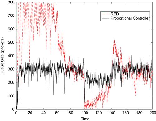
Figure 3.11 compares the performance of the RED and proportional controllers, and we can see that the latter has much faster response time and also lower queue size fluctuations in equilibrium.
3.4.1.3 Proportional-Integral (PI) Controllers
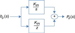
Integral controllers have the property that the steady-state buffer occupancy error is zero. It is possible to design an integral controller for AQM that can clamp the queue size to some reference value regardless of the load value. The simplest of such integral controllers is the PI controller, which is given by the transfer function (Figure 3.12):
The transfer function for the system with the PI controller is given by
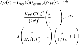 (81)
(81)and in the frequency domain
The following choice of parameters guarantees stability of the PI controlled system:
Choose the zero z of the PI controller as
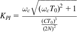
and choose the critical frequency ![]() as
as
where ![]() is chosen to set the PM in a later step. If KPI is chosen as
is chosen to set the PM in a later step. If KPI is chosen as
 (84)
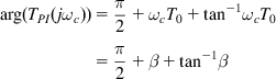
(84)so that it cancels out the high loop gain caused by TCP’s window dynamics, then it follows that ![]() , and hence to show stability, it is sufficient to show that
, and hence to show stability, it is sufficient to show that ![]() radians. Note that
radians. Note that
 (85)
(85)If ![]() is chosen to be in the range
is chosen to be in the range ![]() , then from equation 85, it follows that
, then from equation 85, it follows that ![]() radians. For example, if
radians. For example, if ![]() , then the PM is given by PM=30°.
, then the PM is given by PM=30°.
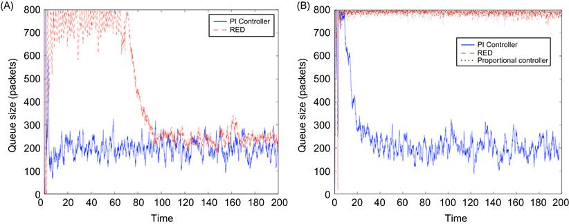
Figure 3.13A [7] shows the result of a simulation with a bottleneck queue size of 800 packets, in which the reference b0 of the PI controller was set to 200 packets and the traffic consisted of a mixture of http and ftp flows. It clearly shows the faster response time PI compared with the RED controller as well as the regulation of the buffer occupancy to the target size of 200 packets. Figure 3.13B shows the case when the number of flows has been increased to the point that the system is close to its capacity. Neither RED nor the proportional controllers are able to stabilize the queue because high packet drop rates have pushed the operating point beyond the size of the queue. The PI controller continues to exhibit acceptable performance, although its response time is a little slower.
The transfer function of the PI controller is described in the s domain in equation 80. For a digital implementation, this description needs to be converted into a z-transform. Using a standard bilinear transform and with the choice of a sampling frequency fs that has to be 10 to 20 times the loop bandwidth, equation 80 can be transformed to the following
The input into the controller is ![]() , and the output is
, and the output is ![]() . Assuming P0=0, it follows from (86) that
. Assuming P0=0, it follows from (86) that
This equation can be converted into a difference equation, so that at time t=kS, where S=1/fs
This equation can also be written as
Hence, when the system converges (i.e., P(kS) becomes approximately equals to P((k−1)S)) both ![]() and
and ![]() go to zero, which implies that the queue length has converged to the reference value b0, and the derivative of the queue length has converged to zero. By equation 55, a zero derivative implies that that input rate of the flows to the bottleneck node exactly matches the link capacity so that there is no up or down fluctuation in the queue level.
go to zero, which implies that the queue length has converged to the reference value b0, and the derivative of the queue length has converged to zero. By equation 55, a zero derivative implies that that input rate of the flows to the bottleneck node exactly matches the link capacity so that there is no up or down fluctuation in the queue level.
The idea of providing difference+derivative AQM feedback has proven to be very influential and constitutes part of the standard toolkit for congestion control designers today. Recently designed algorithms such the IEEE Quantum Congestion Notification (QCN) protocol (see Chapter 8) and XCP/RCP (see Chapter 5), use this idea to stabilize their system.
Despite its superior stability properties, the implementation of PI controllers in TCP/IP networks faces the hurdle that the TCP packet header allows for only 1 bit of congestion feedback. The more recently designed IEEE QCN protocol has implemented a PI controller using 6 bits of congestion feedback in the packet header [15] and is described in Chapter 8.
3.5 The Averaging Principle (AP)
The discussion in Section 3.4 showed that to improve stability for the congestion control algorithm, the network needs to provide information about both the deviation from a target buffer occupancy and the derivative of the deviation. This puts the burden of additional complexity on the network nodes. In practice, this is more difficult to implement than when compared with adding additional functionality to the end systems instead. In this section, we will describe an ingenious way the source algorithm can be modified without touching the nodes, which has the same effect as using a PI-type AQM controller. This is done by applying the so-called Averaging Principle (AP) to the source congestion control rules [16].
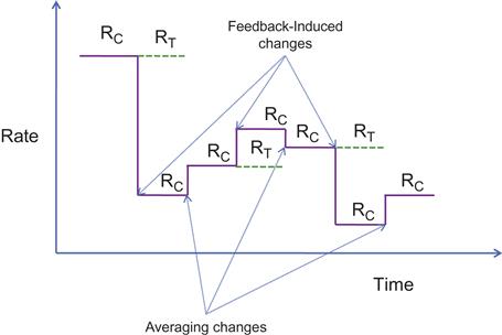
The AP is illustrated in Figure 3.14. It shows a congestion control algorithm, in which the rate reacts to two factors:
1. Periodically once every ![]() seconds, the source changes the transmit rate RC, either up or down, based on the feedback it is getting from the network.
seconds, the source changes the transmit rate RC, either up or down, based on the feedback it is getting from the network.
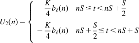
2. At the midpoint between two network-induced rate changes, the source changes its rate according to the following rule: Let RT be the value of the rate before the last feedback-induced change. Then ![]() time units after every feedback induced change, the AP controller performs an “averaging change” when the rate RC is changed as follows:
time units after every feedback induced change, the AP controller performs an “averaging change” when the rate RC is changed as follows:
It can be shown that there exists an AQM controller of the type that was derived in Section 3.4, given by (see Figure 3.15)
such that the AP controller is exactly equivalent to this controller.
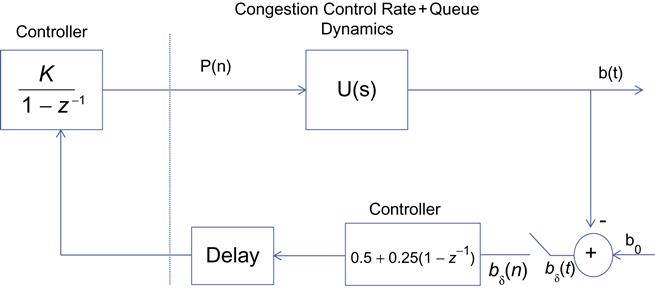
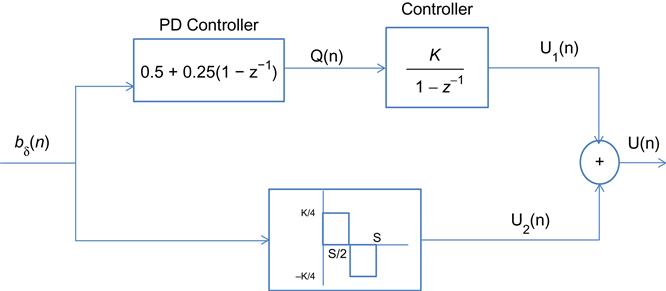
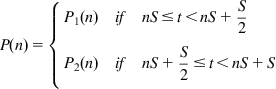
To prove this, consider the following two controllers shown in Figures 3.16 and 3.17. Both controllers map a sequence of sampled queue error samples ![]() to an input signal P(n) that drives the congestion control rate determination function. Controller 1 is an AP controller, and the upper branch of controller 2 is the AQM controller from Figure 3.17. In the following, we will show that P(n)=U(n) and that the lower branch of controller 2 can be ignored, so that
to an input signal P(n) that drives the congestion control rate determination function. Controller 1 is an AP controller, and the upper branch of controller 2 is the AQM controller from Figure 3.17. In the following, we will show that P(n)=U(n) and that the lower branch of controller 2 can be ignored, so that ![]() .
.
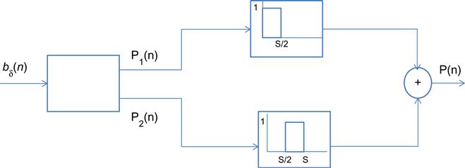
The following equations describe the input-out relations for the two controllers.
 (93)
(93)Controller 2 (approximate PD controller):
 (96)
(96)From equations 91 and 92, it follows that
 (99)
(99)
We now show that
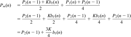
To prove equation 100, note that from equations 99 and 91, it follows that
To prove equation 101, first note from equations 99 and 92 that
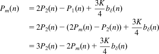
Comparing equations 100 and 101 with equations 96 and 97, it follows that if we can show U1(n)=Pm(n), then it follows that U(n)=P(n), and the two controllers will be equivalent. This can be done by showing that U1(n) and Pm(n) satisfy the same recursions.
From equations 99, 101, and 95, it follows that
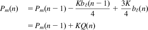 (102)
(102)
Comparing equations 102 and 94, it follows that Pm(n)=U1(n) for all n, and as a consequence we get P(n)=U(n) (i.e., the two controllers are equivalent). Because the contribution of U2(n) can be ignored [16], it follows that ![]() , and the AQM and AP controllers are almost identical.
, and the AQM and AP controllers are almost identical.
We will encounter congestion control protocols such a TCP BIC later in the book (see Chapter 5) that are able to operate in a stable manner in very high-speed networks even with traditional AQM schemes. These protocols may owe their stability to the fact that their rate control rules incorporate averaging of the type discussed here.
3.6 Implications for Congestion Control Algorithms
From the analysis in the previous few sections, a few broad themes emerge that have influenced the design of congestion control algorithms in recent years:
• AQM schemes that incorporate the first or higher derivatives of the buffer occupancy process lead to more stable and responsive systems. This was shown to be the case in the analysis of the PI controller. Also, because the first derivative of the buffer occupancy process can be written as
it also follows that knowing the derivative is equivalent to knowing how close the queue is to its saturation point C. Some protocols such as QCN (see Chapter 8) feed back the value of db/dt directly, and others such as XCP and RCP (see Chapter 5) feed back the rate difference in the RHS of the equation.
• If the network cannot accommodate sophisticated AQM algorithms (which is the case for TCP/IP networks), then an AP-based algorithm can have an equivalent effect on system stability and performance as the derivative-based feedback. Examples of algorithms that have taken this route include the BIC and CUBIC algorithms (see Chapter 5) and QCN (see Chapter 8).
3.7 Further Reading
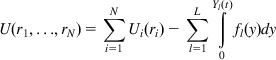
Instead of taking the dual approach to solving equations 7 and 8 it is possible to solve the primal problem directly by eliminating the rate constraint condition (equation 8) and modifying the objective function as follows [9]:
 (103)
(103)
where Ui(ri) are strictly concave functions and the increasing, continuous function fl is interpreted as a congestion price function at link l and the convex function ![]() is known as the barrier function. To impose the constraint that the sum of the data rates at a link should be less than the link capacity, the barrier function can be chosen in a way such that it increases to infinity when the arrival rate approaches the link capacity.
is known as the barrier function. To impose the constraint that the sum of the data rates at a link should be less than the link capacity, the barrier function can be chosen in a way such that it increases to infinity when the arrival rate approaches the link capacity.
It follows that U(r1,…,rN) is a strictly concave function and it can be shown that the problem
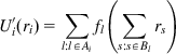
decomposes into N separate optimization subproblems that can be solved independently at each of the sources. The solution to the optimization problem at each source node is given by
 (105)
(105)
where Ai is the set of nodes that connection i passes through and Bl is the set of connections that pass through node l. This can be interpreted as a congestion feedback of ![]() back to the source from each of the nodes that the connection passes through, and is the equivalent of equation 11 for the dual problem.
back to the source from each of the nodes that the connection passes through, and is the equivalent of equation 11 for the dual problem.
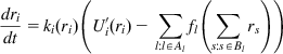
Just as we used the gradient projection method to obtain an iterative solution to the dual problem (equation 13), we can also apply this technique to iteratively solve the primal problem, leading to the following expression for the optimal rates:
 (106)
(106)
where kr is any nondecreasing continuous function such that kr(x)>0 for x>0. If kr>0, then in equilibrium setting, dri/dt=0 leads back to equation 105. Equation 106 is known as the primal algorithm for the congestion control problem. For example, equation 33 for TCP Reno for small values of Qi can be put in the form
which is in the form (106) with
Equation 38 for the utility function can then be obtained using equation 107.
A very good description of the field of optimization and control theory applied to congestion control is given in Srikant’s book [9]. It has a detailed discussion of the barrier function approach to system optimization, as well as several examples of the application of the Nyquist criterion to various types of congestion control algorithms.
For cases when the system equilibrium point falls on a point on nonlinearity, the linearization technique is no longer applicable. In this case, techniques such as Lyapunov’s second theorem have been applied to study system stability.
Appendix 3.A Linearization of the Fluid Flow Model
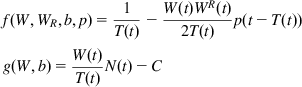
The right-hand sides of the fluid flow model for TCP congestion control that analyzed Section 3.4 are as follows:
 (A1)
(A1)
where ![]() , WR(t)=W(t−T(t)) and TR(t)=T(t−T(t)).
, WR(t)=W(t−T(t)) and TR(t)=T(t−T(t)).
We wish to linearize these equations about their equilibrium points
This can be done using the perturbation formula
By using straightforward differentiation, it can be shown that
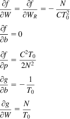 (A4)
(A4)
Substituting equation A4 back into equations A2 and A3 and then into the original differential equation, we obtain the linearized equations
 (A5)
(A5)
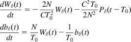
Appendix 3.B The Nyquist Stability Criterion
The Nyquist criterion is used to study the stability of systems that can modeled by linear differential equations in the presence of a feedback loop. In Figure 3.B1, G(s) is the Laplace transform of the system being controlled, and H(s) is the Laplace transform of the feedback function. It can be easily shown that the end-to-end transform for this system is given by
To ensure stability, all the roots of the equation 1+G(s)H(s)=0, which in general are complex numbers, have to lie in the left half of the complex plane. The Nyquist criterion is a technique for verifying this condition that is often easier to apply than finding the roots, and it also provides additional insights into the problem.
Nyquist criterion: Let C be a close contour that encircles the right half of the complex plane, such that no poles or zeroes of H(s)G(s) lie on C. Let Z and P denote the number of poles and zeroes, respectively, of H(s)G(s) that lie inside C. Then the number of times M that ![]() encircles the point (−1,0) in the clockwise direction, as
encircles the point (−1,0) in the clockwise direction, as ![]() is varied from
is varied from ![]() , is equal to Z – P.
, is equal to Z – P.
Note that the contour C in the procedure described above is chosen so that it encompasses the right half of the complex plane. As ![]() is varied from
is varied from ![]() , the function
, the function ![]() maps these points to the target complex plane, where it describes a curve. For the system to be stable, we require that Z=0, and because M=Z – P, it follows that:
maps these points to the target complex plane, where it describes a curve. For the system to be stable, we require that Z=0, and because M=Z – P, it follows that:
• If P=0, then stability requires that M=0, that is, there should no clockwise encirclements of the point (−1,0) by the locus of ![]() .
.
• If P>0, then M=−P, i.e., the locus of ![]() should encircle the point (−1,0) P times in the counterclockwise direction.
should encircle the point (−1,0) P times in the counterclockwise direction.
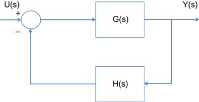
Figure 3.B2 shows an example of the application of the Nyquist criterion to the function ![]() along with some important features. Note that curve for
along with some important features. Note that curve for ![]() goes to
goes to ![]() as
as ![]() , and approaches 0 as
, and approaches 0 as ![]() . We will use the notation
. We will use the notation ![]() , where
, where ![]() is the length of the line going from the origin to
is the length of the line going from the origin to ![]() and
and ![]() is the angle that this line makes with the real axis. Note the following features in the graph:
is the angle that this line makes with the real axis. Note the following features in the graph:
• The point (−a, 0) where the ![]() curve intersects with the real axis is called the phase crossover point because at this point
curve intersects with the real axis is called the phase crossover point because at this point ![]() . The gain margin (GM) of the system is defined by the distance between the phase crossover point and the (−1, 0), i.e.,
. The gain margin (GM) of the system is defined by the distance between the phase crossover point and the (−1, 0), i.e.,
• As the Gain Margin decreases, the system tends towards instability.
• The point where the ![]() curve intersects with the unit circle is called the gain crossover point because at this point
curve intersects with the unit circle is called the gain crossover point because at this point ![]() . The phase margin (PM) of the system is defined by the angle between the crossover point and the negative real axis. Just as for the GM, a smaller PM means that the system is tending toward instability. Generally a PM of between 30 and 60 degrees is preferred.
. The phase margin (PM) of the system is defined by the angle between the crossover point and the negative real axis. Just as for the GM, a smaller PM means that the system is tending toward instability. Generally a PM of between 30 and 60 degrees is preferred.
In the applications of the Nyquist criterion in this book, we usually find a point ![]() such that
such that ![]() . This implies that the gain crossover point
. This implies that the gain crossover point ![]() is such that
is such that ![]() . Hence, if we can prove that
. Hence, if we can prove that ![]() , then the system will be stable.
, then the system will be stable.
Appendix 3.C Transfer Function for the RED Controller
In this appendix, we derive the expression for the transfer function of the RED controller [17], which is diagrammed in Figure 3.C1 and is given by
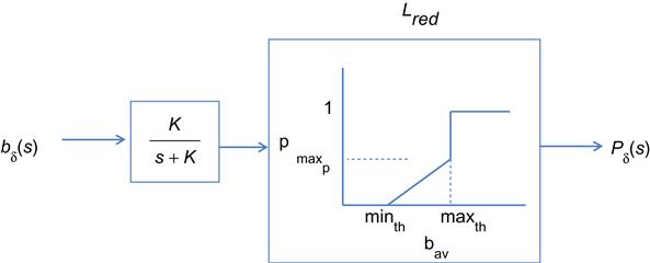
We start with the following equation that describes the operation of the queue averaging process
where ![]() is instantaneous queue length at the sampling time
is instantaneous queue length at the sampling time ![]() and
and ![]() is the average queue length at that time. Assume that this difference equation can be put in the form of the following differential equation
is the average queue length at that time. Assume that this difference equation can be put in the form of the following differential equation
Then, in a sampled data system, x(tk+1) can be written
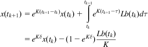 (C2)
(C2)Comparing (C1) with (C2), it follows that L=−K and
Hence, the differential equation for the averaging process is given by ![]() , which in the transform space translates into
, which in the transform space translates into
This signal is further passed through the thresholding process as shown in Figure 3.B1 before yielding the final output that is fed back to the source.
Note that K determines the responsiveness of the filter so higher the value of K, the faster it will respond to sudden change. However, too high a value for K will result in the situation in which the filter starts tracking the instantaneous value of the buffer size, resulting in continuous oscillations.
Appendix 3.D Convex Optimization Theory
Definition 1
A set C is said to be convex if the following property holds:
Definition 2
Define the function ![]() , where
, where ![]() is a convex set. The function is said to be convex if
is a convex set. The function is said to be convex if
The function is said to be concave if
The function is said to be strictly convex (concave) if the above inequalities are strict when ![]() .
.
Consider the following optimization problem:
subject to
where f(x) is a differentiable concave function and P and Q are matrices. The values of x that satisfy the constraints (D3b) form a convex set.
The Lagrangian function L for this problem is defined by
where ![]() are called the dual variables or the Lagrangian multipliers for this problem.
are called the dual variables or the Lagrangian multipliers for this problem.
Karush-Kuhn-Tucker theorem: x is a solution to the optimization problem (D3a–b) if and only if it satisfies the following conditions:
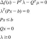 (D5)
(D5)
Definition 3
Define the dual function ![]() by
by
where C is the set of all x that satisfy the constraints (D3b).
Strong Duality Theorem: Let ![]() be the point that solves the constrained optimization problem (equations D3a and D3b). If the Slater constraint qualification conditions are satisfied, then
be the point that solves the constrained optimization problem (equations D3a and D3b). If the Slater constraint qualification conditions are satisfied, then
Appendix 3.E A General Class of Utility Functions
Consider a network with K connections and define the following utility function for connection k [10], given by
for some ![]() , where r is the steady state throughput for connection k. Note that the parameters
, where r is the steady state throughput for connection k. Note that the parameters ![]() controls the trade-off between fairness and efficiency. Consider the following special cases for
controls the trade-off between fairness and efficiency. Consider the following special cases for ![]() :
:
This utility function assigns no value to fairness and simply measures total throughput.
This network resource allocation that minimizes this utility function is known as weighted proportionally fair. The logarithmic factor means that an algorithm that minimizes this function will cut down one user’s allocation by half as long as it can increase another user’s allocation by more than half. The TCP Vegas algorithm has been shown to minimize this utility function.
The network resource allocation corresponding to this utility function is called weighted minimal potential delay fair, and as shown in this chapter, this is function TCP Reno minimizes. This metric seeks to minimize the total time of fixed-length file transfers.
Minimizing this metric is equivalent to achieving max-min fairness in the network [9].