Optimization and Control Theoretic Analysis of Congestion Control
In this chapter, optimization theory and control theory are applied to a differential equation–based fluid flow model of the packet network. This results in the decomposition of the global optimization problem into independent optimizations at each source node, and the explicit derivation of the optimal source rate control rules as a function of a network-wide utility function. In the case of TCP Reno, the source rate control rules are known, but then the theory can be used to derive the network utility function that TCP Reno optimizes. In addition to the mathematical elegance of these results, the results of this theory have been used recently to obtain optimal congestion control algorithms using machine learning techniques. The system stability analysis techniques using the Nyquist criterion, which is introduced in this chapter, have become an essential tool in the study of congestion control algorithms. By using a linear approximation to the delay-differential equation describing the system dynamics, this technique enables us to derive explicit conditions on system parameters to achieve a stable system.
Keywords
congestion control and optimization theory; congestion control and optimal control theory; fluid flow model of congestion control; congestion control and Nyquist stability; congestion control Lagrangian optimization; congestion control dual optimization problem; congestion control primal optimization problem; Active Queue Management; AQM; Random Early Detection; RED; proportional controller; proportional plus integral controller; the averaging principle; TCP utility function
3.1 Introduction
In this chapter, we introduce a network wide model of congestion control in the fluid limit and use it to ask the following questions: Can the optimal congestion control laws be derived as a solution to an optimization problem? If so, what is the utility function being optimized? What is meant by stability of this system, and what are the conditions under which the system is stable? This line of investigation was pursued by Kelly [1], Kelly et al. [2], Low [3], Low et al. [4], Kunniyur and Srikant [5], and Holot et al. [6,7], among others, and their results form the subject matter of this chapter.
As in Chapter 2, we continue to use fluid flow models for the system. Unlike the models used in Chapter 2, the models in this chapter are used to represent an entire network with multiple connections. These models are analogous to the “mean field” models in physics, in which phenomena such as magnetism are represented using similar ideas. They enable the researcher to capture the most important aspects of the system in a compact manner, such that the impact of important system parameters can be analyzed without worrying about per-packet level details.
It has been shown that by applying Lagrangian optimization theory to a fluid flow model of the network, it is possible to decompose the global optimization problem into independent local optimization problems at each source. Furthermore, the Lagrangian multiplier that appears in the solution can be interpreted as the congestion feedback coming from the network. This is an elegant theoretical result that provides a justification for the way congestion control protocols are designed. Indeed, TCP can be put into this theoretical framework by modeling it in the fluid limit, and then the theory enables us to compute the global utility function that TCP optimizes. Alternately, we can derive new congestion control algorithms by starting from a utility function and then using the theory to compute the optimal rate function at the source nodes.
The fluid flow model can also be used to answer questions about TCP’s stability as link speeds and round trip latencies are varied. This is done by applying tools from classical optimal control theory to a linearized version of the differential equations obeyed by the congestion control algorithm. This technique leads to some interesting results, such as the fact that TCP Reno with Active Queue Management (AQM) is inherently unstable, especially when a combination of high bandwidth and large propagation delay is encountered. This analysis has been used to analyze the Random Early Detection (RED) controller and discover suitable parameter settings for it. It has also been used to find other controllers that perform better than RED.
The techniques developed in this chapter for analyzing TCP constitute a useful toolkit that can be used to analyze other congestion control algorithms. In recent years, algorithms such as Data Canter TCP (DCTCP) and the IEEE 802.1 Quantum Congestion Notification (QCN) have been analyzed using these methods. We end the chapter with a discussion of a recent result called the averaging principle (AP), which shows the equivalence of a proportional-integral (PI) type AQM and a special type of rate control rule at the source.
The rest of this chapter is organized as follows: In Section 3.2, we use Lagrangian optimization theory to analyze the congestion control problem and derive an expression for the utility function for TCP Reno. In Section 3.3, we introduce and analyze Generalized additive increase/multiplicative decrease (GAIMD) algorithms, Section 3.4 discusses the application of control theory to the congestion control problem and the derivation of system stability criteria, and Section 3.5 explores a recent result called the AP that has proven to be very useful in designing congestion control algorithms.
An initial reading of this chapter can be done in the following sequence: 3.1→3.2→3.4 (3.4.1 and 3.4.1.1), which covers the basic results needed to understand the material in Part 2 of the book. The most important concepts covered in these sections are that of the formulation of congestion control as the solution to an optimization problem and the application of classical Nyquist stability criteria to congestion control algorithms. More advanced readers can venture into Sections 3.3, 3.4.1.2, 3.4.1.3, and 3.5, which cover the topics of GAIMD algorithms, advanced AQM controllers, and the AP.
3.2 Congestion Control Using Optimization Theory
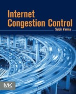
Consider a network with L links and N sources (Figure 3.1).
Ci: Capacity of the ith link, for 1≤i≤L![]() , it is the ith element of the column vector C
, it is the ith element of the column vector C
Li: Set of links that are used by source i
Xli: Element of a routing LXN matrix X, such that Xli=1, if l∈Li![]() , and 0 otherwise
, and 0 otherwise
Ri(t): Transmission rate of source i, for 1≤i≤N![]()
ri: Steady-state value of Ri(t)
Yl(t): Aggregate rate at link l from all the N sources, for 1≤l≤L![]()
yl: Steady-state value of Yi(t)
Pl(t): Congestion measure at link l, for 1≤l≤L![]() . This is later identified as the buffer occupancy at the link.
. This is later identified as the buffer occupancy at the link.
pl: Steady-state value of Pl(t)
τfli(t)![]() : Propagation+Transmission+Queuing delay between the ith source and link l, in the forward direction
: Propagation+Transmission+Queuing delay between the ith source and link l, in the forward direction
τbli(t)![]() : Propagation+Transmission+Queuing delay between the ith source and link l, in the backward direction
: Propagation+Transmission+Queuing delay between the ith source and link l, in the backward direction
Ti(t)=τfli(t)+τbli(t)![]() Total round trip delay
Total round trip delay
Qi(t): Aggregate of all congestion measures for source i, along its route for 1≤i≤N![]()
Note that
Yl(t)=∑Ni=1XliRi(t−τfli(t)),1≤l≤L,and (1)
Qi(t)=∑Ll=1XliPl(t−τbli(t)),1≤i≤N (2)
In steady state,
y=Xrandq=XTp. (3)
Assume that the equilibrium data rate is given by
ri=fi(qi),1≤i≤N (4)
where fi is a positive, strictly monotone decreasing function. This is a natural assumption to make because if the congestion along a source’s path increases, then it should lead to a decrease in its data rate.
Define
Ui(ri)=∫rif−1i(ri)drisothatdUi(ri)dri=f−1i(ri)for1≤i≤N (5)
Because Ui has a positive increasing derivative, it follows that it is monotone increasing and strictly concave.
By construction, the equilibrium rate ri is the solution to the maximization problem
maxri[Ui(ri)−riqi]. (6)
This equation has the following interpretation: If Ui(ri) is the utility that the source attains as a result of transmitting at rate ri, and qi is price per unit data that it is charged by the network, then Equation 6 leads to a maximization of a source’s profit.
Note that Equation 6 is an optimization carried out by each source independently of the others (i.e., the solution ri is individually optimal). We wish to show that ri is also the solution to the following global optimality problem:
maxr≥0∑Ni=1Ui(ri),subjectto (7)
Xr≤C. (8)
Equations 7 and 8 constitute what is known as the primal problem. A unique maximizer, called the primal optimal solution, exists because the objective function is strictly concave, and the feasible solution set is compact. A fully distributed implementation to solve the optimality problem described by equations 7 and 8 is not possible because the sources are coupled to each other through the constraint equation 8).
There are two ways to approach this problem:
1. By modifying the objective function (equation 7) for the primal problem, by adding an extra term called the penalty or barrier function, or
2. By solving the problem that is dual to that described by equations 7 and 8.
In this chapter, we pursue the second option and solve the dual problem (we will briefly describe the solution based on the primal problem in Section 3.7). It can be shown that the solution to the primal problem leads to a direct feedback of buffer-related data without any averaging at the nodes, and the solution to the dual problem leads to processing at the nodes before feedback of more explicit information [1]. In general, we will show that the dual problem leads to congestion feedback that is proportional to the queue size at the congested node, and hence is more appropriate for modeling congestion control systems with AQM algorithms operating at the nodes.
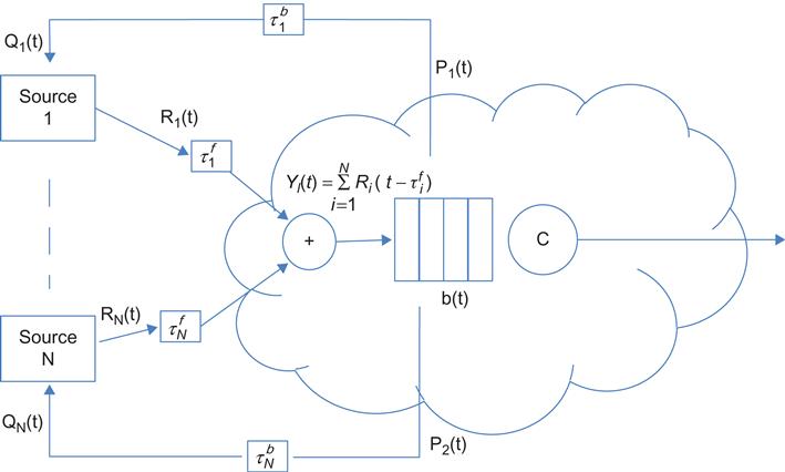
The duality method is a way to solve equations 7 and 8 (Appendix 3.D), which naturally leads to a distributed implementation, as shown next. Let λi![]() be the Lagrange multipliers and define the Lagrangian L(r,λ
be the Lagrange multipliers and define the Lagrangian L(r,λ![]() ) for equations 7 and 8 by
) for equations 7 and 8 by
L(r,λ)=∑Ni=1Ui(ri)−∑Ll=1λl(yl−Cl)=∑Ni=1Ui(ri)−∑Ll=1λl∑Ni=1Xliri+∑Ll=1λlCl=∑Ni=1Ui(ri)−∑Ni=1ri∑Ll=1Xliλl+∑Ll=1λlCl=∑Ni=1[Ui(ri)−ˉqiri]+∑Ll=1λlClwhere (9)
 (9)
(9)
ˉqi=∑Ll=1Xliλl1≤i≤N
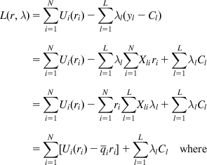
The dual function is defined by
D(λ)=maxri≥0L(r,λ)=∑Ni=1maxri≥0[Ui(ri)−ˉqiri]+∑Ll=1λlCl (10)
 (10)
(10)
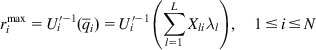
Note that the values
rmaxi=Ui′−1(ˉqi)=Ui′−1(∑Ll=1Xliλl),1≤i≤N (11)
 (11)
(11)
that maximize L(r,λ)![]() , can be computed separately by each source without the need to coordinate with the other sources, in N separate subproblems. However, as equation 11 shows, a source needs information from the network, in the form of ˉqi
, can be computed separately by each source without the need to coordinate with the other sources, in N separate subproblems. However, as equation 11 shows, a source needs information from the network, in the form of ˉqi![]() , before it can compute its optimum rate. Hence, to complete the solution we need to solve the dual problem (i.e., find λl,1≤l≤L
, before it can compute its optimum rate. Hence, to complete the solution we need to solve the dual problem (i.e., find λl,1≤l≤L![]() ) such that
) such that
minλ≥0D(λ) (12)
and substitute them into the equation 11 for rmaxi![]() . The convex duality theorem then states that the optimum rmaxi
. The convex duality theorem then states that the optimum rmaxi![]() computed in equation 10 also maximize the original primal problem (equation 7).
computed in equation 10 also maximize the original primal problem (equation 7).
The dual problem (equation 12) can be solved using the gradient projection method [8], such that
λn+1l=[λnl−γ∂D(λ)∂λl]+ (13)
where γ>0![]() is the step size and [z]+=max{z,0}. From equation 10, it follows that
is the step size and [z]+=max{z,0}. From equation 10, it follows that
∂D(λ)∂λl=Cl−∑Ni=1Xlirmaxi=Cl−yl(rmax),1≤l≤L (14)
Substituting equation 14 back into equation 13, we get
λn+1l=[λnl+γ(yl(rmaxi)−Cl)]+ (15)
Note that the Lagrange multipliers λl![]() behave as a congestion measure at the link because this quantity increases when the aggregate traffic rate at the link yl(rmax) exceeds the capacity Cl of the link and conversely decreases when the aggregate traffic falls below the link capacity. Hence, it makes sense to identify the Lagrange multipliers λl
behave as a congestion measure at the link because this quantity increases when the aggregate traffic rate at the link yl(rmax) exceeds the capacity Cl of the link and conversely decreases when the aggregate traffic falls below the link capacity. Hence, it makes sense to identify the Lagrange multipliers λl![]() with the link congestion measure pl, so that λl=pl,1≤l≤L
with the link congestion measure pl, so that λl=pl,1≤l≤L![]() , and
, and
pn+1l=[pnl+γ(yl(rmaxi)−Cl)]+ (16a)
or in the fluid limit
dpldt={γ(yl(t)−Cl)ifpl(t)>0γ(yl(t)−Cl)+ifpl(t)=0 (16b)
Equations 11 and 16 constitute the solutions to the dual problem. This solution can be implemented in a fully distributed way at the N sources and L links, in the following way:
1. Link l obtains an estimate of the total rate of the traffic from all sources that pass through it, yl.
2. It periodically computes the congestion measure pl![]() using equation 16a, and this quantity is communicated to all the sources whose route passes through link l. This communication can either explicit as in ECN schemes or implicit as in random packet drops with RED.
using equation 16a, and this quantity is communicated to all the sources whose route passes through link l. This communication can either explicit as in ECN schemes or implicit as in random packet drops with RED.
1. Source i periodically computes the aggregate congestion measure for all the links which lie along its route given by
qni=∑Ll=1Xlipnl (17)
2. Source i periodically chooses its new rate using the formula
rni=Ui′−1(qni) (18)
From equations 17 and 18, we obtain the rate control equations for the congestion control problem, if the utility function Ui is known. This distributed procedure is strongly reminiscent of the way TCP congestion control operates, and hence it will not come as a surprise that it can be put into this framework. Hence, TCP congestion control can be interpreted as a solution to the problem of maximizing a global network utility function (equation 7) under the constraints (equation 8). In the next section, we obtain expressions for the utility function U for TCP Reno.
Note that for the case γ=1![]() , equation 16b is precisely the equation satisfied by the queue size process at the node; hence, the feedback variable pl(t) can be identified as the queue size at link l. AQM type schemes can also be put in this framework, as explained next.
, equation 16b is precisely the equation satisfied by the queue size process at the node; hence, the feedback variable pl(t) can be identified as the queue size at link l. AQM type schemes can also be put in this framework, as explained next.
The RED algorithm can be described as follows: Let bl be the queue length at node l and let blav be its average; then they satisfy the following equations:
bn+1l=[bnl+ynl−Cl]+bav,n+1l=(1−αl)bav,nl+αlbnl (19)
In the fluid limit, these become
dbl(t)dt={yl(t)−Clifbl(t)>0[yl(t)−Cl]+ifbl(t)=0 (20)
and
dbavl(t)dt=−αlCl(sl(t)−bavl(t)) (21)
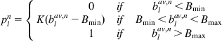
for some constant 0≤α≤1![]() . Then the dropping probability pl is given by
. Then the dropping probability pl is given by
pnl={0ifbav,nl<BminK(bav,nl−Bmin)ifBmin<bav,nl<Bmax1ifbav,nl>Bmax (22)
 (22)
(22)
If we ignore the queue length averaging and let Bmin=0 and consider only the linear portion of equation 22, then the dropping probability becomes
pnl=Kbnl (23)
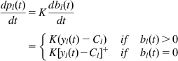
This is referred to as a proportional controller and is discussed further in Section 3.4.1.2 of this chapter. Taking the fluid limit and using equation 20, we get
dpl(t)dt=Kdbl(t)dt={K(yl(t)−Cl)ifbl(t)>0K[yl(t)−Cl]+ifbl(t)=0 (24)
 (24)
(24)
But equation 24 is exactly in the form (equation 16b) that was derived from the gradient projection method for minimizing the dual problem. Hence, a proportional controller–type RED arises as a natural consequence of solving the dual problem at the network nodes.
3.2.1 Utility Function for TCP Reno
There are two ways in which the theoretical results from Section 3.2 can be used in practice:
• Given the system dynamics and the source rate function f (equation 4), compute the network utility function U (equation 5) that this rate function optimizes.
• Given a network utility function U, find the system dynamics and the source rate function that optimizes this utility function.
In this section, we use the first approach, in which a fluid model description for TCP Reno is used to derive the network utility function that it optimizes. We start by deriving an equation for the TCP Reno’s window dynamics in the fluid limit.
Note that the total round trip delay is given by
Ti(t)=Di+∑lXlibl(t)Cl (25)
where Di=Tid+Tiu![]() is the total propagation delay and bl(t) is the ith queue length at time t. The source i rate Ri(t) at time t is defined by
is the total propagation delay and bl(t) is the ith queue length at time t. The source i rate Ri(t) at time t is defined by
Ri(t)=Wi(t)Ti(t) (26)
Using the notation from Section 3.2.1, the aggregate congestion measure Qi(t) at a source can be written as
Qi(t)=1−∏l∈Li(1−Pl(t−τbli(t)))≈∑l∈LiPl(t−τbli(t)) (27)
because it takes τbli(t)![]() seconds for the ACK feedback from link l to reach back to source i. Note that equation 27 is in the form required in equation 2. The aggregate flow rate at link l is given by
seconds for the ACK feedback from link l to reach back to source i. Note that equation 27 is in the form required in equation 2. The aggregate flow rate at link l is given by
Yl(t)=∑lXliRi(t−τfli(t)) (28)
because it takes τfli(t)![]() seconds for the data rate at source i to reach link l.
seconds for the data rate at source i to reach link l.
The rate of change in window size at source i for TCP Reno is then given by the following equation in the fluid limit:
dWi(t)dt=Ri(t−Ti(t))[1−Qi(t)]Wi(t)−Ri(t−Ti(t))Qi(t)124Wi(t)3 (29)
The first term on the Right Hand Side (RHS) of equation 29 captures the rate of increase in window size, which is the rate at which positive ACKs return to the source multiplied by the increase in window size caused by each such ACK during the congestion avoidance phase. The second term captures the rate of decrease of the window size when the source gets positive congestion indications from the network (the factor 4/3 is added to account for the small-scale fluctuation of Wi(t); see Low [3]). Note that equation 29 ignores the change in window size caused by timeouts.
We now make the following approximations: We ignore the queuing delays in equation 25 so that the round trip delay is now fixed and approximated by
Ti=Di+∑lXliCl (30)
The throughput is then approximated by
Ri(t)≈Wi(t)Ti. (31)
It follows from (29) and (31) that
dRi(t)dt≈Ri(t−Ti)[1−Qi(t)]Ri(t)T2i−2Ri(t)Ri(t−Ti)Qi(t)3 (32)
We now assume that Ri(t)≈Ri(t−Ti), so that equation 32 reduces to
dRi(t)dt≈[1−Qi(t)]T2i−2R2i(t)Qi(t)3 (33)
Note that we ignored the propagation delays in the simplifications that led to equation 33. However, modeling these delays is critical in doing a stability analysis of the system, which we postpone to Section 3.4.
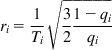
In steady state, it follows from equation 33 that
ri=1Ti√321−qiqi (34)
 (34)
(34)
so that we again recovered the square-root formula. Its inverse is given by
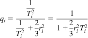
qi=1T2i1T2i+23r2i=11+23r2iT2i (35)
 (35)
(35)
which is in the form postulated in equation 4. From equation 5, it follows that the utility function for TCP Reno is given by
Ui(ri)=∫1T2i(1T2i+23r2i)dri=√3/2Titan−1(√23riTi) (36)
 (36)
(36)
Note that for small values of qi, equation 34 reduces to the expression that is familiar from Chapter 2
ri=1Ti√32qi (37)
 (37)
(37)
If equation 37 is used in equation 5 instead of equation 34, then
qi=32r2iT2i
and the utility function assumes the simpler form
Ui(ri)=−1.5T2iri (38)
Equation 38 is of the form
Ui(ri)=−wiriwithwi=1T2i (39)
Utility functions of the form equation 39 are known to lead to rates that minimize “potential delay fairness” in the network (Appendix 3.E), that is, they minimize the overall potential delay of transfers in progress.
If the utility function is of the form
Ui(ri)=wilogri (40)
then it maximizes the “proportional fairness” in the network. It can be shown that TCP Vegas’s utility function is of the form (40)[9] hence it achieves proportional fairness.
A utility function of type
Ui(ri)=limα→∞r1−αi1−α (41)
leads to a max-min fair allocation of rates [10]. Max-min fairness is in some sense the ideal way of allocating bandwidth in a network; however, in general, it is difficult to achieve max-min fairness using AIMD type algorithms. It can be achieved by using explicit calculations at the network nodes, as was done by the ATM ABR scheme.
The theory developed in the previous two sections forms a useful conceptual framework for designing congestion control algorithms. In Chapter 9, we discuss the recent application of these ideas to the design of congestion control algorithms, which also uses techniques from machine learning theory.
3.3 Generalized TCP–Friendly Algorithms
In this section, we use the theory developed in Section 3.2 to analyze a generalized version of the TCP congestion control algorithm with nonlinear window increment–decrement rules, called GAIMD. We then derive conditions on the GAIMD parameters to ensure that if TCP GAIMD and Reno pass through a bottleneck link, then they share the available bandwidth fairly. This line of investigation was originally pursued to design novel congestion control algorithms for traffic sources such as video, which may not do well with TCP Reno.
αs(Rs(t))![]() : Rule for increasing the data rate in the absence of congestion
: Rule for increasing the data rate in the absence of congestion
βs(Rs(t))![]() : Rule for decreasing the rate in the presence of congestion
: Rule for decreasing the rate in the presence of congestion
Then the rate dynamics is governed by the following equation:
dRs(t)dt=(1−Qs(t))Rs(t−Ts)αs(Rs(t))−Qs(t)Rs(t−Ts)βs(Rs(t)) (42)
Comparing equation 42 with equation 32, it follows that for TCP Reno,
αs(Rs)=1RsT2sandβs(Rs)=Rs2 (43)
From equation 42, it follows that in equilibrium,
qs=αs(rs)αs(rs)+βs(rs)=fs(rs) (44)
so that the utility function for GAIMD is given by
Us(rs)=∫αs(rs)αs(rs)+βs(rs)drs (45)
Define an algorithm to be TCP-friendly if its utility function coincides with that of TCP Reno. From equations 44 and 35, it follows that an algorithm with increase–decrease functions given by (αs,βs)![]() is TCP friendly if and only if
is TCP friendly if and only if
αs(rs)αs(rs)+βs(rs)=22+r2sT2si.e.αs(rs)βs(rs)=2r2sT2s (46)
Following Bansal and Balakrishnan [11], we now connect the rate increase–decrease rules to the rules used for incrementing and decrementing the window size.
Consider a nonlinear window increase–decrease function parameterized by integers (k,l) and constants (α,β)![]() and of the following form (these rules are applied on a per RTT basis):
and of the following form (these rules are applied on a per RTT basis):
W←W+αWkOnpositiveACK (47a)
W←W−βWlOnpacketdrop (47b)
Equations 47a and 47b are a generalization of the AIMD algorithm to nonlinear window increase and decrease and hence are known as GAIMD algorithms. For (k,l)=(0,1), we get AIMD; for (k,l)=(−1,1), we get multiplicative increase/multiplicative decrease (MIMD); for (k,l)=(−1,0), we get multiplicative increase/additive decrease (MIAD); and for (k,l)=(0,0), we get additive increase/additive decrease (AIAD).
Using the same arguments as for TCP Reno, the window dynamics for this algorithm are given by
dWs(t)dt=(1−Qs(t))Rs(t−T)αWk+1s(t)−Qs(t)Rs(t−Ts)βWls(t)
Substituting Ws(t)=Rs(t)Ts![]() , it follows that
, it follows that
dRs(t)dt=(1−Qs(t))Rs(t−Ts)αRk+1s(t)Tk+2s−Qs(t)R(t−Ts)βRls(t)Tl−1s (48)
Comparing this equation with equation 42, we obtain the following expressions for the rate increase–decrease functions for the GAIMD source that corresponds to equations 47a and 47b:
αs(rs)=αrk+1sTk+2sandβs(rs)=βrlsTl−1s (49)
Substituting equation 49 back into the TCP friendliness criterion from equation 46 yields
αβ1(rsTs)k+l+1=2r2sT2s (50)
Hence, the algorithm is TCP friendly if and only if
k+l=1andαβ=2 (51)
Note that if l<1, then this implies that window is reduced less drastically compared with TCP on detection of network congestion. Using equation 51, it follows that in this case, 0<k<1, so that the window increase is also more gradual as compared with TCP.
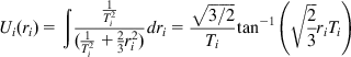
If equate dRs/dt=0 in equilibrium, then we obtain the following expression, which is the analog of the square-root formula for GAIMD algorithms:
rs=(αβ)1/k+l+11Ts(1q1/k+l+1s−1)≈(αβ)1/k+l+11Ts1q1/k+l+1s (52)
 (52)
(52)
Note that the condition k+l=1 also leads to the square root law for TCP throughput.
3.4 Stability Analysis of TCP with Active Queue Management
The stability of a congestion control system is defined in terms of the behavior of the bottleneck queue size b(t). If the bottleneck queue size fluctuates excessively and very frequently touches zero, thus leading to link under utilization, then the system is considered to be unstable. Also, if the bottleneck queue size grows and spends all its time completely full, which leads to excessive packet drops, then again the system is unstable. Hence, ideally, we would like to control the system so that the bottleneck queue size stays in the neighborhood of a target length, showing only small fluctuations.
It has been one of the achievements of fluid modeling of congestion control systems that it makes it possible to approach this problem by using the tools of classical control system theory. This program was first carried out by Vinnicombe [12] and Holot et al. [6,7] The latter group of researchers modeled TCP Reno, for which they analyzed the RED controller, and another controller that they introduced called the PI controller. Since then, the technique has been applied to many other congestion control algorithms and constitutes one of the basic techniques in the toolset for analyzing congestion control.
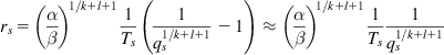
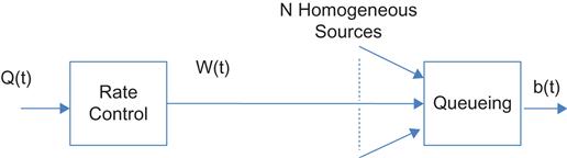
To analyze the stability of the system, we will follow Holot and colleagues [6,7] and use a simplified model shown in Figure 3.2. In particular, we assume that there are N homogeneous TCP sources, all of which pass through single bottleneck node.
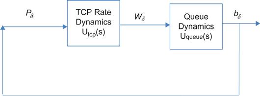
Initially, let’s consider the open-loop system shown in Figure 3.3. Later in this and subsequent sections, we will connect the queue length process b(t) with congestion indicator process Q(t), using a variety of controllers. Using equation 29, its window control dynamics are given by
dW(t)dt=R(t−T(t))[1−Q(t)]W(t)−R(t−T(t))W(t)Q(t)2 (53)
and substitute W(t)=R(t)T(t) in the first term on the RHS and make the approximations R(t)≈R(t−T(t)),1−Q(t)≈1![]() , leading to the equation
, leading to the equation
dW(t)dt=1T(t)−W(t)W(t−T(t))2T(t−T(t))Q(t) (54)
where T(t)=b(t)C+D![]() .
.
The fluid approximation for the queue length process at the bottleneck can be written as
db(t)dt=W(t)T(t)N(t)−C (55)
Equations 54 and 55 give the nonlinear dynamics for the rate control and queuing blocks, respectively, in Figure 3.3. To simplify the optimal control problem so that we can apply the techniques of optimal control theory, we now proceed to linearize these equations. With (W(t), b(t)), and Q(t) as the input, the operating point (W0, Q0,P0) is defined by dW/dt=0 and db/dt=0, which leads to
dWdt=0⇒W20Q0=2 (56)
dbdt=0⇒W0=CT0N (57)
where
T0=b0C+DasperEquation25 (58)
Assuming N(t)=N and T(t)=T0 as constants, equations 54 and 55 can be linearized around the operating points (W0, b0, Q0) (Appendix 3.A), resulting in
dWδ(t)dt=−2NCT20Wδ(t)−C2T02N2Qδ(t) (59)
dbδ(t)dt=NT0Wδ(t)−1T0bδ(t) (60)
where
Wδ=W−W0bδ=b−b0Qδ=Q−Q0

The Laplace transforms of equations 59 and 60 are given by
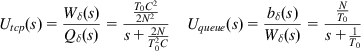
Utcp(s)=Wδ(s)Qδ(s)=T0C22N2s+2NT20CUqueue(s)=bδ(s)Wδ(s)=NT0s+1T0 (61)
 (61)
(61)
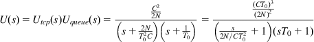
so that the Laplace transform of the plant dynamics for the linearized TCP+queuing system is
U(s)=Utcp(s)Uqueue(s)=C22N(s+2NT20C)(s+1T0)=(CT0)3(2N)2(s2N/CT20+1)(sT0+1) (62)
 (62)
(62)
and it relates the change in the packet marking probability Qδ![]() to the change in queue size bδ
to the change in queue size bδ![]() .
.
System stability can be studied with the help of various techniques from optimal control theory, including Nyquist plots, Bode plots, and root locus plots [13]. Of these, the Nyquist plot is the most amenable to analyzing systems with delay lags of the type seen in these systems and hence is used in this chapter. Appendix 3.B has a quick introduction to the topic of the Nyquist stability criterion that the reader may want to consult at this point.
Assuming initially that there is no controller present, so that there is no AQM stabilization and the queue size difference is fed back to the sender with no delay, then the system is as shown in Figure 3.5, so that Qδ=Pδ=bδ![]() :
:
From Equation 62, the open loop transfer function of this system is of the form
U(s)=K(as+1)(bs+1)
with a,b>0. The corresponding close loop transfer function W(s) is given by
W(s)=U(s)1+U(s)=K(as+1)(bs+1)+K.
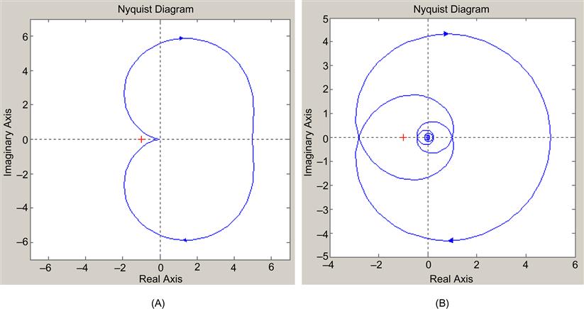
Using the Nyquist criterion, we can see that the locus of U(jω)![]() as ω
as ω![]() varies from 0 to ∞
varies from 0 to ∞![]() , does not encircle the point (−1, 0), even for large values of K; hence, the system is unconditionally stable (see Figure 3.4A).
, does not encircle the point (−1, 0), even for large values of K; hence, the system is unconditionally stable (see Figure 3.4A).
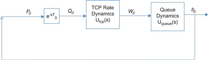
Next let’s introduce the propagation delay into the system, so that Qδ(t)=Pδ(t−T)![]() , as shown in Figure 3.6. In this case, equation 59 changes to
, as shown in Figure 3.6. In this case, equation 59 changes to
dWδ(t)dt=−2NCT20Wδ(t)−C2T02N2Pδ(t−T)
This introduction of the delay in the feedback loop can lead to system instability, as shown next.
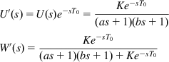
The open loop and closed loop transfer functions for this system are given by
U′(s)=U(s)e−sT0=Ke−sT0(as+1)(bs+1)W′(s)=Ke−sT0(as+1)(bs+1)+Ke−sT0
From the Nyquist plot for U′(jω)![]() shown in Figure 3.4B, note the following:
shown in Figure 3.4B, note the following:
• The addition of the delay component has led to a downward spiraling effect in the locus of U′(jω)![]() . This is because U′(jω)=|U′(jω)|e−jarg(U′(jω))
. This is because U′(jω)=|U′(jω)|e−jarg(U′(jω))![]() where the point (ω,U′(jω))
where the point (ω,U′(jω))![]() on the curve makes the following angle with the real axis:
on the curve makes the following angle with the real axis:
arg(U′(jω))=ωT0+tan−1aω+tan−1bω![]()
Hence, as ω![]() increases, the first term on the RHS increases linearly, and the other two terms are limited to at most π2
increases, the first term on the RHS increases linearly, and the other two terms are limited to at most π2![]() each.
each.
• The system is no longer unconditionally stable, and as the gain K increases, it may encircle the point (−1,0) in the clockwise direction, thus rendering it unstable.
From equation 62, the gain K for TCP Reno is given by
K=(CT0)3(2N)2
so that the system can become unstable in the presence of feedback if either (1) C increases or (2) T0 increases or if N decreases. Thus, this proves that high link capacity or high round trip latency can cause system instability.
Although the onset of instability with increasing C or T0 is to be expected, the variation with N implies that the system gains in stability with more sessions. The intuitive reason for this is that more sessions average out the fluctuations because of the high variations in TCP window size (especially the decrease by half on detecting congestion). With only a few sessions, these variations affect the stability of the system because even a single packet drop causes a large drop in window size. On the other hand, with many connections, the decrease in window size of any one of them does not have as large an effect. Some of the high-speed variations of TCP that we will meet in Chapter 5 reduce their windows by less than half on detecting packet loss, thus reducing K and subsequently increasing their stability in the presence of large C and T0.
3.4.1 The Addition of Controllers to the Mix
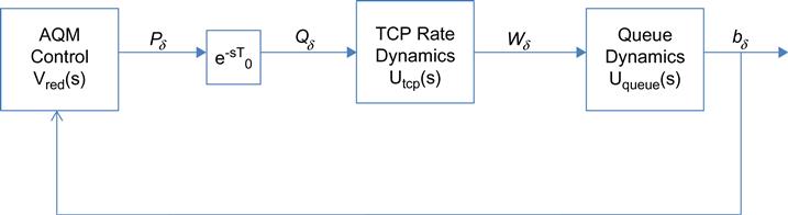
Because the system shown in Figure 3.6 can become unstable, we now explore the option of adding a controller into the loop, as shown in Figure 3.7, and then adjusting the controller parameters in order to stabilize the system. We will first analyze the RED controller, and then based on the learning from its analysis, introduce two other controllers, the Proportional and the PI controllers, that are shown to have better performance than the RED controller.
3.4.1.1 Random Early Detection (RED) Controllers
The RED controller is shown in Figure 3.8, and its Laplace transform is given by (see Appendix 3.C for a derivation)
Vred(s)=LredsK+1where (63)
Lred=maxpmaxth−minthandK=−log(1−wq)δ (64)
where wq is the weighing factor used to smoothen out the queue size estimate and δ![]() is the queue size sampling frequency, which is set to 1/C. The other RED parameters are defined in Section 1.4.2 in Chapter 1. As Figure 3.8 shows, the RED controller consists of a Low Pass Filter (LPF) followed by a constant gain.
is the queue size sampling frequency, which is set to 1/C. The other RED parameters are defined in Section 1.4.2 in Chapter 1. As Figure 3.8 shows, the RED controller consists of a Low Pass Filter (LPF) followed by a constant gain.
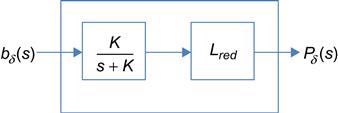
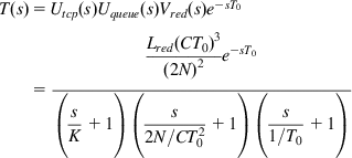
The objective of the optimal control problem is to choose RED parameters Lred and K to stabilize the system shown in Figure 3.7. Note that the open loop transfer function for the system is given by
T(s)=Utcp(s)Uqueue(s)Vred(s)e−sT0=Lred(CT0)3(2N)2e−sT0(sK+1)(s2N/CT20+1)(s1/T0+1) (65)
 (65)
(65)
To apply the Nyquist criterion, set s=jω![]() , so that
, so that
T(jω)=|T(jω)|e−jarg(T(jω))![]() where
where
|T(jω)|=Lred(CT0)3(2N)2√(ωK)2+1√(ω2N/CT20)2+1√(ω1/T0)2+1and (66)
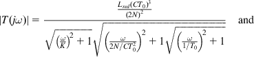 (66)
(66)
arg(T(jω))=ωT0+tan−1ωK+tan−1ω2N/CT20+tan−1ω1/T0 (67)
Holot et al. [6] proved the following result:
Let Lred and K satisfy:
Lred(T+C)3(2N−)2≤√ω2cK2+1where (68)
ωc=0.1min{2N−(T+)2C,1T+} (69)
then the linear feedback control system in Figure 3.7 using a RED controller is stable for all N≥N−![]() and all T0≤T+
and all T0≤T+![]() .
.
To prove this, we start with the following observation: From equation 66, it follows that
|T(jω)|≤Lred(CT0)3(2N)2√(ωK)2+1 (70)
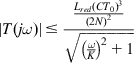 (70)
(70)
Furthermore, if ω=ωc,N≥N−,T0≤T+![]() , then it follows from equations 68 and 70 that
, then it follows from equations 68 and 70 that
|T(jωc)|≤1 (71)
From this, we conclude that the critical frequency ω*![]() at which |T(jω*)|=1
at which |T(jω*)|=1![]() , satisfies the relation ω*≤ωc
, satisfies the relation ω*≤ωc![]() (this is because |T(jω)|
(this is because |T(jω)|![]() is monotonically decreasing in ω
is monotonically decreasing in ω![]() ). Hence, it follows from the Nyquist criterion that if we can show that the angle argT(jωc)
). Hence, it follows from the Nyquist criterion that if we can show that the angle argT(jωc)![]() satisfies the condition
satisfies the condition
argT(jωc)<πradians (72)
then the system has a positive phase margin (PM) given by
PM≥π−argT(jωc)>0