Introduction
This chapter is an introduction to the subject of congestion control and covers some basic results in this area, such as the Chiu-Jain result on the optimality of additive increase/multiplicative decrease (AIMD) control and descriptions of fundamental congestion control algorithms such as TCP Reno, TCP Vegas, and Random Early Detection (RED)–based Active Queue Management (AQM). A detailed description of TCP Reno is provided, including algorithms such as Congestion Avoidance, Fast Retransmit and Fast Recovery, Slow Start, and TCP Timer operation. AQM techniques are introduced, and the RED algorithm is described.
Keywords
Congestion Control definition and objectives; TCP Reno; TCP Vegas; Active Queue Management; AQM; Random Early Detection; RED; Congestion Avoidance; Fast Retransmit; Fast Recovery; Slow Start
1.1 Introduction
The Transmission Control Protocol (TCP) is one of the pillars of the global Internet. One of TCP’s critical functions is congestion control, and the objective of this book is to provide an overview of this topic, with special emphasis on analytical modeling of congestion control protocols.
TCP’s congestion control algorithm has been described as the largest human-made feedback-controlled system in the world. It enables hundreds of millions of devices, ranging from huge servers to the smallest PDA, to coexist together and make efficient use of existing bandwidth resources. It does so over link speeds that vary from a few kilobits per second to tens of gigabits per second. How it is able to accomplish this task in a fully distributed manner forms the subject matter of this book.
Starting from its origins as a simple static-window–controlled algorithm, TCP congestion control went through several important enhancements in the years since 1986, starting with Van Jacobsen’s invention of the Slow Start and Congestion Avoidance algorithms, described in his seminal paper [1]. In addition to significant developments in the area of new congestion control algorithms and enhancements to existing ones, we have seen a big increase in our theoretical understanding of congestion control. Several new important application areas, such as video streaming and data center networks (DCNs), have appeared in recent years, which have kept the pace of innovation in this subject area humming.
The objective of this book is twofold: Part 1 provides an accessible overview of the main theoretical developments in the area of modeling of congestion control systems. Not only have these models helped our understanding of existing algorithms, but they have also played an essential role in the discovery of newer algorithms. They have also helped us explore the limits of stability of congestion control algorithms. Part 2 discusses the application of congestion control to some important areas that have arisen in the past 10 to 15 years, namely Wireless Access Networks, DCNs, high-speed links, and Packet Video Transport. Each of these applications comes with its own unique characteristics that has resulted in new requirements from the congestion control point of view and has led to a proliferation of new algorithms in recent years. Several of these are now as widely deployed as the legacy TCP congestion control algorithm. The strong theoretical underpinning that has been established for this subject has helped us greatly in understanding the behavior of these new algorithms.
The rest of this chapter is organized as follows: Section 1.2 provides an introduction to the topic of congestion control in data networks and introduces the idea of additive increase/multiplicative decrease (AIMD) algorithms. Section 1.3 provides a description of the TCP Reno algorithm, and Section 1.4 discusses Active Queue Management (AQM). TCP Vegas is described in Section 1.5, and Section 1.6 provides an overview of the rest of the chapters in this book.
1.2 Basics of Congestion Control
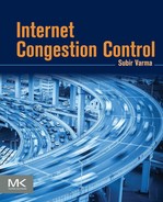
The problem of congestion control arises whenever multiple distributed agents try to make use of shared resources (Figure 1.1). It arises widely in different scenarios, including traffic control on highways or air traffic control. This book focuses on the specific case of packet data networks, where the high-level objective of congestion control is to provide good utilization of network resources and at the same time provide acceptable performance for the users of the network.
The theory and practice of congestion control for data networks have evolved in the past 3 decades to the system that we use today. The early Internet had very rudimentary congestion control, which led to a series of network collapses in 1986. As a result, a congestion control algorithm called TCP Slow Start (also sometimes called TCP Tahoe) was put into place in 1987 and 1988, which, in its current incarnation as TCP Reno, remains one of the dominant algorithms used in the Internet today. Since then, the Internet has evolved and now features transmissions over wireless media, link speeds that are several orders of magnitudes faster, widespread transmission of video streams, and the recent rise of massive data centers. The congestion control research and development community has successfully met the challenge of modifying the original congestion control algorithm and has come up with newer algorithms to address these new types of networks.
1.2.1 The Congestion Control Problem Definition
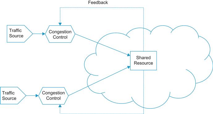
To define the congestion control problem more formally, consider the graph in Figure 1.2 in which the throughput of a data source has been plotted on the y-axis and the network traffic load from the source has been plotted on the x-axis. We observe the following:
• If the load is small, the throughput keeps up with the increasing load. After the load reaches the network capacity, at the “knee” of the curve, the throughput stops increasing. Beyond the knee, as the load increases, queues start to build up in the network, thus increasing the end-to-end latency without adding to the throughput. The network is then said to be in a state of congestion.
• If the traffic load increases even further and gets to the “cliff” part of the curve, then the throughput experiences a rather drastic reduction. This is because queues within the network have increased to the point that packets are being dropped. If the sources choose to retransmit to recover from losses, then this adds further to the total load, resulting in a positive feedback loop that sends the network into congestion collapse.
To avoid congestion collapse, each data source should try to maintain the load it is sending into the network in the neighborhood of the knee. An algorithm that accomplishes this objective is known as a congestion avoidance algorithm; a congestion control algorithm tries to prevent the system from going over the cliff. This task is easier said than done and runs into the following challenge: The location of the knee is not known and in fact changes with total network load and traffic patterns. Hence, the problem of congestion control is inherently a distributed optimization problem in which each source has to constantly adapt its traffic load as a function of feedback information it is receiving from the network as it tries to stay near the knee of the curve.
The original TCP Tahoe algorithm and its descendants fall into the congestion control category because in the absence of support from the network nodes, the only way they can detect congestion is by filling up the network buffers and then detecting the subsequent packet drops as a sign of congestion. Many routers today implement a more sophisticated form of buffer management called Random Early Detection (RED) that provides early warnings of a congestive situation. TCP in combination with RED then qualifies as a congestion avoidance algorithm. Algorithms such as TCP Vegas operate the system around the knee without requiring special support in the network nodes.
Some of the questions that need to be answered in the design of a congestion control algorithm include the following (all of the new terms used below are defined in this chapter):
• Should the congestion control be implemented on an end-to-end or on a hop-by-hop basis?
• Should the traffic control be exercised using a windows-based mechanism or a rate-based mechanism?
• How does the network signal to the end points that it is congested (or conversely, not congested)?
• What is the best Traffic Rate Increment rule in the absence of congestion?
• What is the best Traffic Rate Decrement rule in the presence of congestion?
• How can the algorithm ensure fairness among all connections sharing a link, and what measure of fairness should be used?
• Should the congestion control algorithm prioritize high link utilization of low end-to-end latency?
There is a function closely related to congestion control, called flow control, and often the two terms are used interchangeably. For the purposes of this book, flow control is defined as a function that is used at the destination node to prevent its receive buffers from overflowing. It is implemented by providing feedback to the sender, usually in the form of window-size constraints. Later in this book, we will discuss the case of video streaming in which the objective is to prevent the receive buffer from underflowing. We classify the algorithm used to accomplish this objective also in the flow control category.
1.2.2 Optimization Criteria for Congestion Control
This section and the next are based on some pioneering work by Chiu and Jain [2] in the congestion control area. They defined optimization criteria that the congestion control algorithms should satisfy, and then they showed that there is a class of controls called AIMD that satisfies many of these criteria. We start by enunciating the Chiu-Jain optimization criteria in this section.
Consider a network with N data sources and define ri(t) to be the data rate (i.e., load) of the ith data source. Also assume that the system is operating near the knee of the curve from Figure 1.2 so that the network rate allocation to the ith source after congestion control is also given by ri(t). We assume that the system operation is synchronized and happens in discrete time so that the rate at time (t+1) is a function of the rate at time t, and the network feedback received at time t. We will also assume that the network congestion feedback is received at the sources instantaneously without any delay.
Define the following optimization criteria for selecting the best control:
• Efficiency: Every source has a bottleneck node, which is the node where it gets the least throughput among all the nodes along its path. Let Ai be the set of other sources that also pass through this bottleneck node; then the efficiency criterion states that ![]() should be as close as possible to C, where C is the capacity of the bottleneck node.
should be as close as possible to C, where C is the capacity of the bottleneck node.
• Fairness: The efficiency criterion does not put any constraints on how the data rates are distributed among the various sources. A fair allocation is when all the sources that share a bottleneck node get an equal allocation of the bottleneck link capacity. The Jain fairness index defined below quantifies this notion of fairness.
(1)
Note that this index is bounded between 0 and 1, so that a totally fair allocation (with all ri’s equal) has an index of 1, but a totally unfair allocation (in which the entire capacity is given to one user) has an index of 1/N.
• Convergence: There are two aspects to convergence. The first aspect is the speed with which the rate ri(t) gets to its equilibrium rate at the knee after starting from zero (called responsiveness). The second aspect is the magnitude of its oscillations around the equilibrium value while in steady state (called smoothness).
1.2.3 Optimality of Additive Increase Multiplicative Decrease Congestion Control
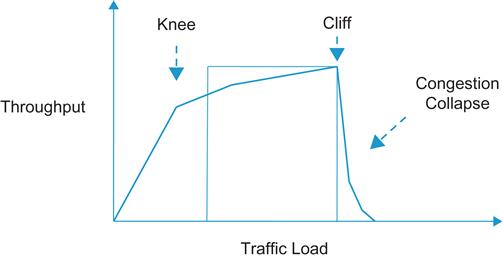
In this section, we restrict ourselves to a two-source network that shares a bottleneck link with capacity C. As shown in Figure 1.3, any rate allocation (r1,r2) can be represented by a point in a two-dimensional space. The objective of the optimal congestion control algorithm is to bring the system close to the optimal point (C/2, C/2) irrespective of the starting position.
We assume that the system evolves in discrete time, such that at the nth step the following linear controls are used:
(3)
Note the following special cases:
• aI=aD=0, bI>1 and 0<bD<1 corresponds to multiplicative increase/multiplicative decrease (MIMD) controls.
• bI=bD=1 corresponds to additive increase/additive decrease (AIAD) controls.
• bI=1, aD=0 and 0<bD<1 corresponds to AIMD controls.
• aI=0, bD=1 corresponds to multiplicative increase/additive decrease (MIAD) controls.
With reference to Figure 1.3, note the following:
• All allocations for which r1+r2=C are efficient allocations, which correspond to points on the “efficiency line” in Figure 1.3. All points below the efficiency line represent underloaded systems, and the correct control decision in this region is to increase the rates. Conversely, all points above the efficiency line represent overloaded systems, and the correct control decision in this region is to decrease the rates.
• All allocations for which r1=r2 are fair allocations, which corresponds to points on the “fairness line” in Figure 1.3. Also note that because the fairness at any point (r1, r2) is given by
multiplying both the rates by a factor b does not change the fairness, that is, (br1, br2) has the same fairness as (r1, r2). Hence all points on the straight line joining (r1, r2) to the origin have the same fairness and such a line is called an “equi-fairness” line.
• The efficiency line and the fairness line intersect at the point (C/2, C/2), which is the optimal operating point.
• The additive increase policy of increasing both users’ allocations by aI corresponds to moving up along a 45-degree line. The multiplicative decrease policy of increasing both users’ allocations by bI corresponds to moving along the line that connects the origin to the current operating point.
Figure 1.3 shows the trajectory of the two-user system starting from point a R0 using an AIMD policy. Because R0 is below the efficiency line, the policy causes an additive increase along a 45-degree line that moves the system to point R1 (assuming a big enough increment value), which is above the efficiency line. This leads to a multiplicative decrease in the next step by moving to point R2 toward the origin on the line that joins R1 to the origin (assuming a big enough decrement value). Note that R2 has a higher fairness index than R0. This increase–decrease cycle repeats over and over until the system converges to the optimal state (C/2, C/2).
Using similar reasoning, it can be easily seen that with both the MIMD or the AIAD policies, the system never converges toward the optimal point but keeps oscillating back and forth across the efficiency line. Hence, these systems achieve efficiency but not fairness. The MIAD system, on the other hand, is not stable and causes one of the rates to blow up over time.
These informal arguments can be made more rigorous [2] to show that the AIMD policy given by
(4)
(5)
is the optimal policy to achieve the criteria defined in Section 1.2.2. Indeed, most of the algorithms for congestion control that are described in this book adhere to the AIMD policy. This analysis framework can also be extended to nonlinear increase–decrease algorithms of the type
(6)
Nonlinear algorithms have proven to be especially useful in the congestion control of high-speed links over large propagation delays, and several examples of this type of algorithm are presented in Chapter 5 of this book.
Two assumptions were made in this analysis that greatly simplified it: (1) the network feedback is instantaneous, and (2) the sources are synchronized with each other and operate in discrete time. More realistic models of the network that are introduced in later chapters relax these assumptions; as a result, the analysis requires more sophisticated tools. The simple equations 2 and 3 for the evolution of the transmit rates have to be replaced by nonlinear delay-differential equations, and the proof of system stability and convergence requires sophisticated techniques from control theory such as the Nyquist criterion.
1.2.4 Window-Based Congestion Control
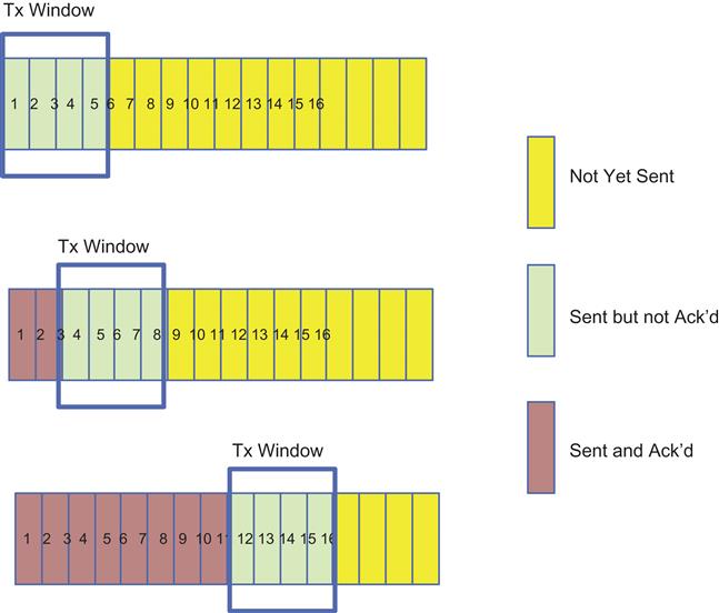
Window-based congestion control schemes have historically preceded rate-based schemes and, thanks to the popularity of TCP, constitute the most popular type of congestion control scheme in use today. As shown in Figure 1.4, a window whose size can be set either in bytes or in multiples of the packet size drives the basic operation. Assuming the latter and a window size of N packets, the system operates as follows:
• Assume that the packets are numbered sequentially from 1 and up. When a packet gets to the destination, an ACK is generated and sent back to the source. The ACK carries the sequence number (SN) of packet that it is acknowledging.
• The source maintains two counters, Ack’d and Sent. Whenever a packet is transmitted, the Sent counter is incremented by 1, and when an ACK arrives from the destination, the Ack’d counter is incremented by 1. Because the window size is N packets, the difference un_ackd=(Sent–Ack’d) is not allowed to exceed N. When unAck’d=N, then the source stops transmitting and waits for more ACKs to arrive.
• ACKs can be of two types: An ACK can either acknowledge individual packets, which is known as Selective Repeat ARQ, or it can carry a single SN that acknowledges multiple packets with lower SNs. The latter strategy is called Go Back N.
This simple windowing scheme with the Go Back N Acking strategy is basically the way in which TCP congestion control operated before 1988.
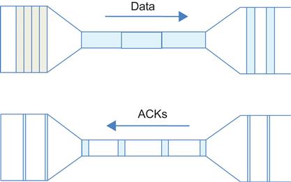
Figure 1.5 illustrates the mechanism by which a simple static window scheme is able to react to congestion in the network. This served as the primary means of congestion control in the Internet before the introduction of the TCP Slow Start algorithm. As shown, if a node is congested, then the rate at which ACKs are sent back is precisely equal to the rate at which the congested node is able to serve the packets in its queue. As a result, the source sending rate gets autoregulated to the rate at which the bottleneck node can serve the packets from that source. This is also known as the “self-clocking” property and is one of the benefits of the window-based congestion control over the rate-based schemes.
The window-based scheme also functions as an effective flow control algorithm because if the destination is running out of buffers, then it can withhold sending ACKs and thereby reduce the rate at which packets are being transmitted in the forward direction.
Readers will notice that there are a number of potential problems with the static window congestion control algorithm. In particular:
1. When the algorithm is started, there is no mechanism to regulate the rate at which the source sends packets into the network. Indeed, the source may send a whole windowfull of packets back to back, thus overwhelming nodes along the route and leading to lost packets. When the ACKs start to flow back, the sending rate settles down to the self-clocked rate.
2. Given a window size of W and a round trip time of T, the average throughput R is given by the formula R=W/T in steady state (this is explained in Chapter 2). If the network is congested at a node, then the only way to clear it is by having the sources traversing that node reduce their sending rate. However, there is no way this can be done without reducing the corresponding window sizes. If we do introduce a mechanism to reduce window sizes in response to congestion, then we also need to introduce a complementary mechanism to increase window sizes after the congestion goes away.
3. If the source were to vary its window size in response to congestion, then there needs to be a mechanism by which the network can signal the presence of congestion back to the source.
Partially as a result of a lack of mechanism to address the first two issues, the Internet suffered a so-called “congestion collapse” in 1986, during which all traffic ground to a halt. As a result, a number of proposals made by Van Jacobsen and Karels [1] were adopted that addressed these shortcomings. These are described in detail in Section 1.3.
1.2.5 Rate-Based Congestion Control
Instead of using a window to regulate the rate at which the source is sending packets into the network, the congestion control algorithm may alternatively release packets using a packet rate control mechanism. This can be implemented by using a timer to time the interpacket intervals. In practice, the end-to-end rate-based flow control (EERC) algorithm, which was part of the Asynchronous Transfer Mode (ATM) Forum Available Bit Rate (ABR) traffic management scheme, was one instance when a rate-based control was actually put into practice [3]. However, because ABR was not widely implemented in even ATM networks, there is less practical experience with rate-based schemes than with dynamic window schemes. More recently, rate-based control has been used for the TCP Friendly Rate Control (TFRC) algorithm, which is used for streaming applications. Video streaming was thought to be an area in which rate-based control fits in more naturally than window-based control. However, even for video, the industry has settled on a scheme that uses TCP for congestion control for reasons that are explained in Chapter 6. Rate control has been used in recent years in non-TCP contexts, and a couple of examples of this are provided in this book: The IEEE802.1Qau algorithm, also known as Quantum Congestion Notification (QCN; see Chapter 8), uses rate-based control, and so does the Google Congestion Control (GCC; see Chapter 9) algorithm that is used for real-time interbrowser communications.
Compared with window-based schemes, rate-based schemes have the following disadvantages:
• Window-based schemes have a built-in choke-off mechanism in the presence of extreme congestion when the ACKs stop coming back. However, in rate-based schemes, there is no such cut-off, and the source can potentially keep pumping data into the network.
• Rate-based schemes require a more complex implementation at both the end nodes and in the network nodes. For example, at the end node, the system requires a fine-grained timer mechanism to control the rates.
1.2.6 End-to-End versus Hop-by-Hop Congestion Control
In the discussion thus far, we have implicitly assumed that the congestion control mechanism exists on an end-to-end basis (i.e., other than providing congestion feedback, the network nodes do not take any other action to relieve the congestion). However, there exists an alternate design called hop-by-hop congestion control, which operates on a node-by-node basis. Such a scheme was actually implemented as part of the IBM Advanced Peer to Peer Network (APPN) architecture [4] and was one of the two competing proposals for the ATM ABR congestion control algorithm [3].
Hop-by-hop congestion control typically uses a window-based congestion control scheme at each hop and operates as follows: If the congestion occurs at the nth node along the route and its buffers fill up, then that node stops sending ACKs to the (n-1)rst node. Because the (n-1)rst node can no longer transmit, its buffers will start to fill up and consequently will stop sending ACKs to the (n-2)nd node. This process continues until the backpressure signal reaches the source node. Some of the benefits of hop-by-hop congestion control are:
• Hop-by-hop schemes can do congestion control without letting the congestion deteriorate to the extent that packets are being dropped.
• Individual connections can be controlled using hop-by-hop schemes because the window scheme described earlier operated on a connection-by-connection basis. Hence, only the connections that are causing congestion need be controlled, as opposed to all the connections originating at the source node or traversing a congested link.
Note that these benefits require that the hop-by-hop window be controlled on a per-connection basis. This can lead to greater complexity of the routing nodes within the network, which is the reason why hop-by-hop schemes have not found much favor in the Internet community, whose design philosophy has been to push all complexity to the end nodes and keep the network nodes as simple as possible.
The big benefit of hop-by-hop schemes is that they react to congestion much faster than end-to-end schemes, which typically take a round trip of latency or longer. The rise of DCNs, which are very latency sensitive, has made this feature more attractive, and as seen in Chapter 7, some recent data center–oriented congestion control protocols feature hop-by-hop congestion control. Also, hop-by-hop schemes are attractive for systems that cannot tolerate any packet loss. An example of this is the Fiber Channel protocol used in Storage Area Networks (SAN), which is a user of hop-by-hop congestion control.
1.2.7 Implicit versus Explicit Indication of Network Congestion
The source can either implicitly infer the existence of network congestion, or the network can send it explicit signals that it is congested. Both of these mechanisms are used in the Internet. Regular TCP is an example of a protocol that implicitly infers network congestion by using the information contained in the ACKs coming back from the destination, and TCP Explicit Congestion Notification (ECN) is an example of a protocol in which the network nodes explicitly signal congestion.
1.3 Description of TCP Reno
Using the taxonomy from Section 1.2, TCP congestion control can be classified as a window-based algorithm that operates on an end-to-end basis and uses implicit feedback from the network to detect congestion. The initial design was a simple fixed window scheme that is described in Sections 1.3.1 and 1.3.2. This was found to be inadequate as the Internet grew, and a number of enhancements were made in the late 1980s and early 1990s (described in Sections 1.3.3 and 1.3.4), which culminated in a protocol called TCP Reno, which still remains one of the most widely implemented congestion control algorithms today.
1.3.1 Basic TCP Windowing Operations
TCP uses byte-based sequence numbering at the transport layer. The sender maintains two counters:
• Transmit Sequence Number (TSN) is the SN of the next byte to be transmitted. When a data packet is created, the SN field in the TCP header is filled with the current value of the TSN, and the sender then increments the TSN counter by the number of bytes in the data portion of the packet. The number of bytes in a packet is equal to Maximum Segment Size (MSS) and can be smaller if the application runs out of bytes to send.
• Ack’d Sequence Number (ASN) is the SN of the next byte that the receiver is expecting. The ASN is copied from the ACK field of the last packet that is received.
To maintain the window operation, the sender enforces the following rule:
(7)
where W is the transmit window size in bytes and SN is the sequence number of the next packet that sender wishes to transmit. If the inequality is not satisfied, then the transmit window is full, and no more packets can be transmitted.
The receiver maintains a single counter:
• Next Sequence Number (NSN): This is the SN of the next byte that the receiver is expecting. If the SN field of the next packet matches the NSN value, then the NSN is incremented by the number of bytes in the packet. If the SN field in the received packet does not match the NSN value, then the NSN is left unchanged. This event typically happens if a packet is lost in transmission and one of the following packets makes it to the receiver.
The receiver inserts the NSN value into the ACK field of the next packet that is being sent back. Note that ACKs are cumulative, so that if one of them is lost, then the next ACK makes up for it. Also, an ACK is always generated even if SN of a received packet does not match the NSN. In this case, the ACK field will be set to the old NSN again. This is a so-called Duplicate ACK, and as discussed in Section 1.3.4, the presence of Duplicate ACKs can be used by the transmitter as an indicator of lost packets, and indirectly, network congestion.
ACKs are usually piggybacked on the data flowing back in the opposite direction, but if there is no data flowing back, then the receiver generates a special ACK packet with an empty data field. To reduce the number of ACK packets flowing back, most receiver implementations start a 200-msec timer on receipt of a packet, and if another packet arrives within that period, then a single ACK is generated. This rule, which is called Delayed ACKs, cuts down the number of ACKs flowing back by half.
The receiver also implements a receive window (RW), whose value is initially set to the number of bytes in the receive buffer. If the receiver has one or more packets in the receive buffer whose total size is B bytes, then it reduces the RW size to RW=(RW−B). All ACKs generated at the receiver carry the current RW value, and on receipt of the ACK, the sender sets the transmit window to W=min(W, RW). This mechanism, which was referred to as flow control in Section 1.2.1, allows the receiver with insufficient available buffer capacity to throttle the sender.
Note that even though TCP maintains byte counters to keep track of the window sizes, the congestion control algorithms to be described next are often specified in terms of packet sizes. The packet that is used in these calculations is of size equal to the TCP packet size.
1.3.2 Window Size Decrements, Part 1: Timer Operation and Timeouts
The original TCP congestion control algorithm used a retransmit timer as the sole mechanism to detect packet losses and as an indicator of congestion. This timer counts in ticks of 500-msec increments, and the sender keeps track of the number of ticks between when a packet is transmitted and when its gets ACKed. If the value of the timer exceeds the value of the retransmission timeout (RTO), then the sender assumes that the packet has been lost and retransmits it. The sender also takes two other actions on retransmitting a packet:
• The sender doubles the value of RTO and keeps doubling if there are subsequent timeouts for the same packet until it is delivered to the destination.
• The sender reduces the TCP window size to 1 packet (i.e., W=1).
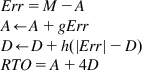
Choosing an appropriate value for RTO is critical because if the value is too low, then it can cause unnecessary timeouts, and if the value is too high, then the sender will take too long to react to network congestion. The current algorithm for RTO estimation was suggested by Jacobsen and Karels [1] and works as follows:
M: Latest measurement of the round trip latency value (RTT). The sender only measures the RTT for one packet at a time. When a timeout and retransmission occur on the packet being used for measurement, then the RTT estimators are not updated for that packet.
D: The smoothed mean deviation of the RTT g, h: Smoothing constants used in the estimate of A and D, respectively. g is set to 0.125 and h to 0.25.
The calculations are as follows:
(8)
 (8)
(8)
Before Jacobsen and Karels’ [1] work, the RTO value was set to a multiple of A alone, which underestimated the timeout value, thus leading to unnecessary retransmissions.
1.3.3 Window Size Increments: Slow Start and Congestion Avoidance
1.3.3.1 Slow Start
The windowing algorithm described in Section 1.3.1 assumed static windows. Among other problems, this led to the scenario whereby on session start-up, a whole window full of packets would be injected at back to back into the network at full speed. This led to packet drops as buffers became overwhelmed. To correct this problem, Jacobsen and Karels [1] proposed the Slow Start algorithm, which operates as follows:
• At the start of a new session, set the TCP transmit window size to W=1 packet (i.e., equal to MSS bytes). The sender sends a packet and waits for its ACK.
• Every time an ACK is received, increase the window size by one packet (i.e., W←W+1).
Even though the algorithm is called Slow Start, it actually increases the window size quite rapidly: W=1 when the first packet is sent. When the ACK for that packet comes back, W is doubled to 2, and two packets are sent out. When the ACK for the second packet arrives, then W is set to 3, and the ACK for the third packet causes W to increase to 4. Hence, during the Slow Start phase, the correct reception of each windowfull of packets causes the W to double (i.e., the increase is exponential) (Figure 1.6). The rapid increase is intentional because it enables the sender to quickly increase its bandwidth to the value of the bottleneck capacity along its path, assuming that the maximum window size is large enough to achieve the bottleneck capacity. If the maximum window size is not large enough to enable to connection to get to the bottleneck capacity, then the window stops incrementing when the maximum window size is reached. Also note that during the Slow Start phase, the receipt of every ACK causes the sender to inject two packets into the network, the first packet because of the ACK itself and second packet because the window has increased by 1.
1.3.3.2 Congestion Avoidance
During normal operation, the Slow Start algorithm described in Section 1.3.3.1 is too aggressive with its exponential window increase, and something more gradual is needed. The congestion avoidance algorithm, which was also part of Van Jacobsen and Karels’ [1] 1988 paper, leads to a linear increase in window size and hence is more suitable. It operates as follows:
1. Define a new sender counter called ssthresh. At the start of the TCP session, ssthresh is initialized to large value, usually 64 KBytes.
2. Use the Slow Start algorithm at session start, which will lead to an exponential window increase, until the bottleneck node gets to the point where a packet gets dropped (assuming that there are enough packets being transmitted for the system to get to this point). Let’s assume that this happens at W=Wf.
3. Assuming that the packet loss is detected because of a timer expiry, then the sender resets the window to W=1 packet (i.e., MSS bytes) and sets ssthresh=Wf/2 bytes.
4. After the session successfully retransmits the lost packet, the Slow Start algorithm is used to increment the window size until W≥ssthresh bytes. Beyond this value, the window is increased using the following rule on the receipt of every ACK packet:
(9)
5. In step 3, if the packet gets dropped because of Duplicate ACKs (these are explained in Section 1.3.4) rather than a timer expiry, then a slightly different rule is used. In this case, the sender sets W=Wf/2 as well as ssthresh=Wf/2. After the lost packet is recovered, the sender directly transitions to the congestion avoidance phase (because W=ssthresh) and uses equation 9 to increment its windows.
Note that as a result of the window increment rule (equation 9), the receipt of ACKs for an entire window full of packets leads to an increase in W by just one packet. Typically, it takes a round trip or more to transmit a window of packets and receive their ACKs; hence, under the congestion avoidance phase, the window increases by at most one packet in every round trip (i.e., a linear increase) (see Figure 1.6) This allows the sender to probe whether the bottleneck node is getting close to its buffer capacity one packet at a time, and indeed if the extra packet causes the buffer to overflow, then at most one packet is lost, which is easier to recover from.
1.3.4 Window Size Decrements, Part 2: Fast Retransmit and Fast Recovery
Section 1.3.3 discusses the rules that TCP Reno uses to increment its window in the absence of network congestion. This section discusses the rules that apply to decrementing the window size in the presence of congestion. TCP uses the design philosophy that dropped packets are the best indicator of network congestion, which falls within the implicit congestion indicator category from Section 1.2.4. When TCP Slow Start was first designed, this was the only feedback that could be expected from the simpler routers that existed at that time. In retrospect, this decision came with a few issues: The only way that the algorithm can detect congestion is by driving the system into a congestive state (i.e., near the cliff of the curve in Figure 1.2). Also, if the packet losses are because of a reason other than congestion (e.g., link errors), then this may lead to unnecessary rate decreases and hence performance loss. This problem is particularly acute for error-prone wireless links, as explained in Chapter 4.
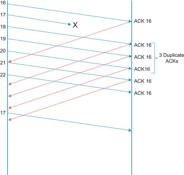
As alluded to in Section 1.3.3.2, TCP uses two different mechanisms to detect packet loss. The first technique uses the retransmit timer RTO and is discussed in Section 1.3.2. The second technique is known as Fast Retransmit (Figure 1.7) and tries to make the system more responsive to packet losses. It works as follows:
• If the SN field in a packet at the receiver does not match the NSN counter, then the receiver immediately sends an ACK packet, with the ACK field set to NSN. The receiver continues to do this on subsequent packets until SN matches NSN (i.e., the missing packet is received).
• As a result of this, the sender begins to receive more than one ACK with the same ACK number; these are known as duplicate ACKs. The sender does not immediately jump to the conclusion that the duplicate ACKs are caused by a missing packet because in some cases, they may be caused by packets getting reordered before reception. However, if the number of duplicate ACKs reaches three, then the sender concludes that the packet has indeed been dropped, and it goes ahead and retransmits the packet (whose SN=duplicate ACK value) without waiting for the retransmission timer to expire. This action is known as Fast Retransmit.
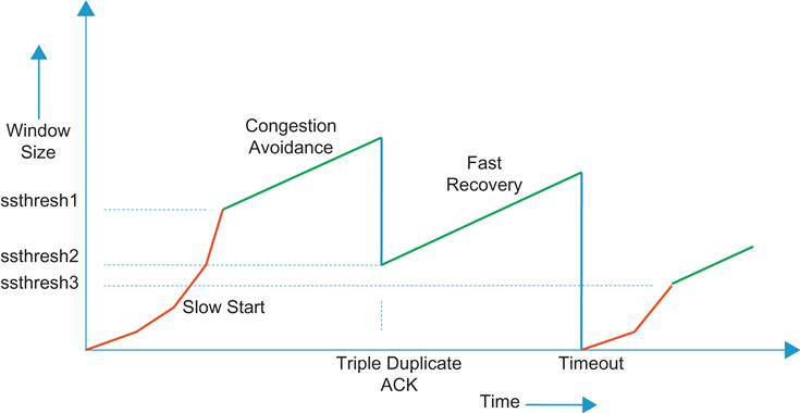
• Just before the retransmission, the sender sets the ssthresh value to half the current window size W, and after the retransmission, it sets W←ssthresh+3.MSS. Each time another duplicate ACK arrives, the sender increases W by the packet size, and if the new value of W allows, it goes ahead and transmits a new packet. This action is known as Fast Recovery.
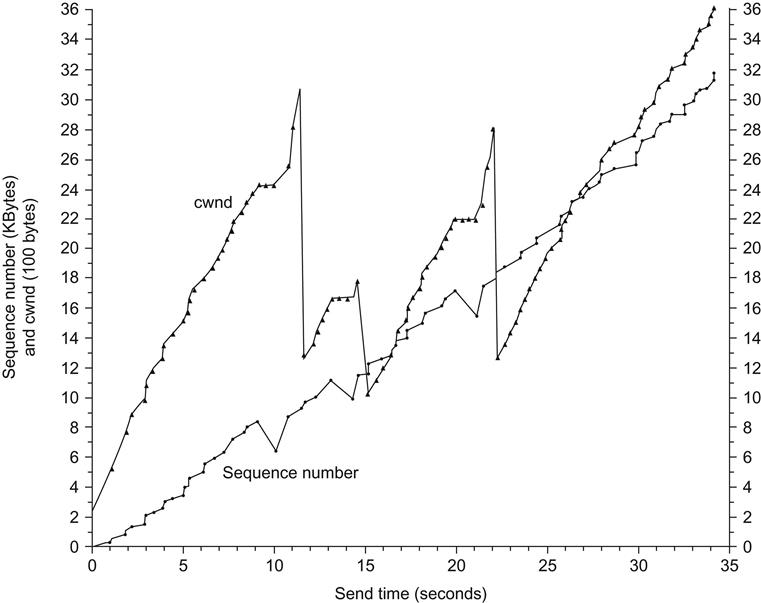
The justification for this is the following: When the receiver finally receives the missing packet, the next ACK acknowledges all the other packets that it has received in the window, which on the average can be half the transmit window size. When the sender receives this ACK, it is allowed to transmit up to half a window of back-to-back packets (because W is now at half the previous value), which can potentially overwhelm the buffers in the bottleneck node. However, by doing FAST Recovery, the sender keeps sending additional packets while it waits for the ACK for the missing packet to arrive, and this prevents the sudden onslaught of new packets into the network. When the ACK for the missing packet arrives, W is set back to the ssthresh value in the previous step. This behavior can be seen in Figure 1.8; note that the window size shows a spike of 3 MSS on error detection and falls back to W/2 after the missing packet is received.
The Fast Retransmit mechanism is able to efficiently recover from packet losses as long as no more than one packet is lost in the window. If more than one packet is lost, then usually the retransmit timer for the second or later expires, which triggers the more drastic step of resetting W back to one packet.
1.3.5 TCP New Reno
Not long after the introduction of TCP Reno, it was discovered that it is possible to improve its performance significantly by making the following change to the Fast Recovery phase of the algorithm: If a Partial ACK is received during the Fast Recovery period that acknowledges some but not all of the packets that were outstanding at the start of the Fast Recovery period, then this is treated as an indication that the packet immediately following the acknowledged packet has also been lost and should be retransmitted. Thus, if multiple packets are lost within a single window, then New Reno can recover without a retransmission timeout by retransmitting one lost packet per round trip until all the lost packets from the window have been retransmitted. New Reno remains in Fast Recovery until all data outstanding at the start of the Fast Recovery phase has been acknowledged.
In this book, we will assume that legacy TCP implies Reno, with the understanding that the system has also implemented the New Reno changes.
1.3.6 TCP Reno and AIMD
Even though it may not be very clear from the description of TCP Reno in the last few sub-sections, this algorithm does indeed fall into the class of AIMD congestion control algorithms. This can be most clearly seen by writing down the equations for the time evolution of the window size.
In the Slow Start phase, as per the description in Section 1.3.3.1, the window size after n round trip times is given by
(10)
where W0 is the initial window size. This equation clearly captures the exponential increase in window size during this phase.
During the Congestion Avoidance phase (Section 1.3.3.2), the window size evolution is given by
(11)
because each returning ACK causes the window size to increase by 1/W, and equation 11 follows from the fact that there are W returning ACKs for a window of size W.
Detection of a lost packet at time t because of Duplicate ACKs causes a reduction in window size by half, so that
(12)
Note that with New Reno, multiple packet losses within a window result in a single reduction in the window size.
The AIMD nature of TCP Reno during the congestion avoidance/fast retransmit phases is clearly evident from equations 11 and 12.
1.4 Network Feedback Techniques
Network feedback constitutes the second half of a congestion control algorithm design and has as much influence in determining the properties of the resulting algorithm as the window or rate control performed at the source. It is implemented using algorithms at a switch or router, and traditionally the design bias has been to make this part of the system as simple as possible to keep switch costs low by avoiding complex designs. This bias still exists today, and even though switch logic is several orders of magnitudes faster, link speeds have increased at the same rate; hence, the cost constraint has not gone away.
1.4.1 Passive Queue Management
The simplest congestion feedback that a switch can send back to the source is by simply dropping a packet when it runs out of buffers, which is referred to as tail-drop feedback. This was how most routers and switches operated originally, and even today it is used quite commonly. Packet loss triggers congestion avoidance at the TCP source, which takes action by reducing its window size.
Even though tail-drop feedback has the virtue of simplicity, it is not an ideal scheme for the following reasons:
• Tail-drop–based congestion signaling can lead to excess latencies across the network if the bottleneck node happens to have a large buffer size. Note that the buffer need not be full for the session to attain full link capacity; hence, the excess packets queued at the node add to the latency without improving the throughput (this claim is proven in Chapter 2).
• If multiple TCP sessions are sharing the buffer at the bottleneck node, then the algorithm can cause synchronized packet drops across sessions. This causes all the affected sessions to reduce their throughput, which leads to a periodic pattern, resulting in underutilization of the link capacity.
• Even for a single session, tail-drop feedback tends to drop multiple packets at a time, which can trigger the TCP RTO–based retransmission mechanism, with its attendant drop in window size to one packet.
An attempt to improve on this led to the invention of RED-based queue management, which is described in the next section.
1.4.2 Active Queue Management (AQM)
To correct the problems with tail-drop buffer management, Floyd and Jacobsen [5] introduced the concept of AQM, in which the routing nodes use a more sophisticated algorithm called RED to manage their queues. The main objectives of RED are the following:
• Provide congestion avoidance by controlling the average queue size at a network node.
• Avoid global synchronization and a bias against bursty traffic sources.
• Maintain the network in a region of low delay and high throughput by keeping the average queue size low while fluctuations in the instantaneous queue size are allowed to accommodate bursty traffic and transient congestion.
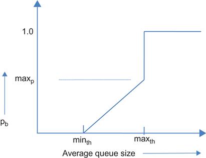
As explained later, RED provides congestion feedback to the source when the average queue size exceeds some threshold, either by randomly dropping a packet or by randomly marking the ECN bit in a packet. Furthermore, the packet dropping probability is a function of the average queue size, as shown in Figure 1.9.
The RED algorithm operates as follows:
1. Calculate the average queue size avg as ![]() , where q is the current queue size. The smoothing constant wq determines the time constant of this low-pass filter. This average is computed every time a packet arrives at the node.
, where q is the current queue size. The smoothing constant wq determines the time constant of this low-pass filter. This average is computed every time a packet arrives at the node.
2. Define constants minth and maxth, such that minth is the minimum threshold for the average queue size and maxth is the maximum threshold for the average queue size (see Figure 1.9). If ![]() , then on packet arrival, calculate the probability pb and pa as
, then on packet arrival, calculate the probability pb and pa as
(13)
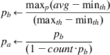 (13)
(13)
where maxp is the maximum value for pb and count is the number of packets received since the last dropped packet. Drop the arriving packet with probability pa. Note that pa is computed such that after each drop, the algorithm uniformly chooses one of the next 1/pb packets to drop next.
This randomized selection of packets to be dropped is designed to avoid the problem of synchronized losses that is seen in tail-drop queues.
RED has been heavily analyzed, with the objective of estimating the optimal queue thresholds and other parameters. Some of this work is covered in Chapter 3, where tools from optimal control theory are brought to bear on the problem. In general, researchers have discovered that RED is not an ideal AQM scheme because there are issues with its responsiveness and ability to suppress queue size oscillations as the link capacity or the end-to-end latency increases. Choosing a set of RED parameters that work well across a wide range of network conditions is also a nontrivial problem, which has led to proposals that adapt the parameters as network conditions change.
However, it is widely implemented in routers today, and furthermore, all the analysis work done on RED has led to the discovery of other more effective AQM schemes. More recent AQM algorithms that build off the ideas in RED include the Data Center Congestion Control Protocol (DCTCP) (see Chapter 7), the IEEE 802.1Qau QCN algorithm (see Chapter 8), and an influential protocol designed for high-speed networks called eXpress Control Protocol (XCP) (see Chapter 5).
Floyd [6] also went on to design a follow on enhancement to RED called ECN. In ECN systems, the queue does not discard the packet but instead marks the ECN bits in TCP packet header. The receiver then receives the marked packets and in turn marks the ECN bit in the returning ACK packet. When the sender receives ACKs with marked packets, then it reacts to them in the same way as if it had detected a lost packet using the duplicate ACK mechanism and proceeds to reduce its window size. This avoids unnecessary packet drops and thus unnecessary delays for packets. It also increases the responsiveness of the algorithm because the sender does not have to wait for three duplicate ACKs before it can react to congestion.
1.5 Delay-Based Congestion Control: TCP Vegas
Brakmo and Peterson [7] proposed a fundamentally different solution to the congestion control problem compared with TCP Reno. Their algorithm, which they called TCP Vegas, uses end-to-end packet delay as a measure of congestion rather than packet drops. This idea has proven to be very influential and has inspired the design of several congestion control protocols that are in wide use today, including Compound TCP (CTCP), which is the default protocol on all Windows servers (see Chapter 5); Low Extra Delay Background Transport (LEDBAT), which is used for background data transfers by the Bit-Torrent file sharing service (see Chapter 4); and FAST TCP, which was designed for high-speed networks (see Chapter 5).
TCP Vegas estimates the level of congestion in the network by calculating the difference in the expected and actual data rates, which it then uses to adjust the TCP window size. Assuming a window size of W and a minimum round trip latency of T seconds, the source computes an expected throughput RE once per round trip delay, by
(14)
The source also estimates the current throughput R by using the actual round trip time Ts according to
(15)
The source then computes the quantity Diff given by
(16)
Note that Diff can also be written as
(17)
By Little’s law [8], the expression on the RHS equals the number of packets belonging to the connection that are queued in the network and hence serves as a measure of congestion.
Define two thresholds ![]() and
and ![]() such that
such that ![]() . The window increase decrease rules are given by:
. The window increase decrease rules are given by:
• When ![]() , then leave W unchanged.
, then leave W unchanged.
• When ![]() , decrease W by 1 for the next RTT. This condition implies that congestion is beginning to build up the network; hence, the sending rate should be reduced.
, decrease W by 1 for the next RTT. This condition implies that congestion is beginning to build up the network; hence, the sending rate should be reduced.
• When ![]() , increase W by 1 for the next RTT. This condition implies the actual throughput is less than the expected throughput; hence, there is some danger that the connection may not use the full network bandwidth.
, increase W by 1 for the next RTT. This condition implies the actual throughput is less than the expected throughput; hence, there is some danger that the connection may not use the full network bandwidth.
TCP Vegas tries to maintain the “right” amount of queued data in the network. Too much queued data will cause congestion, and too little queued data will prevent the connection from rapidly taking advantage of transient increases in available network bandwidth. Note that this mechanism also eliminates the oscillatory behavior of TCP Reno while reducing the end-to-end latency and jitter because each connection tends to keep only a few packets in the network.
A few issues with TCP Vegas were pointed out by Mo and colleagues [9], among them the fact that when TCP Vegas and Reno compete for bandwidth on the same link, then Reno ends with a greater share because it is more aggressive in grabbing buffers, but Vegas is conservative and tries to occupy as little space as it can. Also, if the connection’s route changes (e.g., because of mobility), then this causes problems with Vegas’ round trip latency estimates and leads to a reduction in throughput. Because of these reasons, especially the first one, Vegas is not widely deployed despite its desirable properties.
1.6 Outline of the Rest of the Book
The contents of this book are broadly split in to two parts:
Part 1 is devoted to the analysis of models of congestion control systems.
Chapter 2 has a detailed discussion of TCP models, starting from simple models using fluid approximations to more sophisticated models using stochastic theory. The well-known “square root” formula for the throughput of a TCP connection is derived and is further generalized to AIMD congestion control schemes. These formulae have proven to be very useful over the years and have formed an integral part of the discovery of new congestion control protocols, as shown in Part 2. For example, several high-speed protocols discussed in Chapter 5 use techniques from Chapter 2 to analyze their algorithms. Chapter 2 also analyzes systems with multiple parallel TCP connections and derives expressions for the throughput ratio as a function of the round trip latencies.
Chapter 3 has more advanced material in which optimization theory and optimal control theory are applied to a differential equation–based fluid flow model of the packet network. This results in the decomposition of the global optimization problem into independent optimizations at each source node and the explicit derivation of the optimal source rate control rules as a function of a network wide utility function. In the case of TCP Reno, the source rate control rules are known, but then the theory can be used to derive the network utility function that Reno optimizes. In addition to the mathematical elegance of these results, the results of this theory have been used recently to obtain optimal congestion control algorithms using machine learning techniques (see discussion of Project Remy in Chapter 9). The system stability analysis techniques using the Nyquist criterion introduced in Chapter 3 have become an essential tool in the study of congestion control algorithms and are used several times in Part 2 of this book. By using a linear approximation to the delay-differential equation describing the system dynamics, this technique enables us to derive explicit conditions on system parameters to achieve a stable system.
Part 2 of the book describes congestion control protocols used in five different application area, namely broadband wireless access networks, high-speed networks with large latencies, video transmission networks, DCNs, and Ethernet networks.
Chapter 4 discusses congestion control in broadband wireless networks. This work was motivated by finding solutions to the performance problems that TCP Reno has with wireless links. Because the algorithm cannot differentiate between congestion losses and losses caused by link errors, decreasing the window size whenever a packet is lost has a very detrimental effect on performance. The chapter describes TCP Westwood, which solved this problem by keeping an estimate of the data rate of the connection at the bottleneck node. Thus, when Duplicate ACKs are received, the sender reduces its window size to the transmit rate at the bottleneck node (rather than blindly cutting the window size by half, as in Reno). This works well for wireless links because if the packet was lost because of wireless errors, then the bottleneck rate my still be high, and this is reflected in the new window size. The chapter also describes techniques, such as Split-Connection TCP and Loss Discrimination Algorithms, that are widely used in wireless networks today. The combination of TCP at the end-to-end transport layer and link layer retransmissions (ARQ) or forward error correction (FEC) coding on the wireless link is also analyzed using the results from Chapter 2. The large variation in link capacity that is observed in cellular networks has led to a problem called bufferbloat. Chapter 4 describes techniques using AQM at the nodes as well as end-to-end algorithms to solve this problem.
Chapter 5 explores congestion control in high-speed networks with long latencies. One of the consequences of the application of control theory to TCP congestion control, described in Chapter 3, was the realization that TCP Reno was inherently unstable as the delay-bandwidth product of the network became large or even for very large bandwidths. As a result of this, a number of new congestion control designs were suggested with the objective of solving this problem such as High Speed TCP (HSTCP), TCP BIC, TCP CUBIC, and Compound TCP (CTCP), which are described in the chapter. Currently, TCP CUBIC serves as the default congestion control algorithm for Linux servers and as a result is as widely deployed as TCP Reno. CTCP is used as the default option for Windows servers and is also very widely deployed. The chapter also describes the XCP and RCP algorithms that have been very influential in the design of high-speed congestion control protocols. Finally, the chapter makes connections between the algorithms in this chapter and the stability theory from Chapter 3 and gives some general guidelines to be used in the design of high-speed congestion control algorithms.
Chapter 6 covers congestion control for video streaming applications. With the explosion in video streaming traffic in recent years, there arose a need to protect the network from congestion from these types of sources and at the same time ensure good video performance at the client end. The industry has settled on the use of TCP for transmitting video even though at first cut, it seems to be an unlikely match for video’s real-time needs. This problem was solved by a combination of large receive playout buffers, which can smoothen out the fluctuations caused by TCP rate control, and an ingenious algorithm called HTTP Adaptive Streaming (HAS). HAS runs at the client end and controls the rate at which “chunks” of video data are sent from the server, such that the sending rate closely matches the rate at which the video is being consumed by the decoder. Chapter 6 describes the work in this area, including several ingenious HAS algorithms for controlling the video transmission rate.
Chapter 7 discusses congestion control in DCNs. This is the most current, and still rapidly evolving, area because of the enormous importance of DCNs in running the data centers that underlie the modern Internet economy. Because DCNs can form a relatively autonomous region, there is also the possibility of doing a significant departure from the norm of congestion control algorithms if the resulting performance is worth it. This has resulted in innovations in congestion control such as the application of ideas from Earliest Deadline First (EDF) scheduling and even in-network congestion control techniques. All of these are driven by the need to keep the end-to-end latency between two servers in a DCN to values that are in the tens of milliseconds or smaller to satisfy the real-time needs of applications such as web searching and social networking.
Chapter 8 covers the topic of congestion control in Ethernet networks. Traditionally, Ethernet, which operates at Layer 2, has left the task of congestion control to the TCP layer. However recent developments such as the spread of Ethernet use in applications such as SANs has led the networking community to revisit this design because SANs have a very strict requirement that no packets be dropped. As a result, the IEEE 802.1 Standards group has recently proposed a congestion control algorithm called IEEE802.1Qau or QCN for use in Ethernet networks. This algorithm uses several advances in congestion control techniques described in the previous chapters, such as the use of rate averaging at the sender, as well as AQM feedback, which takes the occupancy as well as the rate of change of the buffer size into account.
Chapter 9 discusses three different topics that are at the frontiers of research into congestion control: (1) We describe a project from MIT called Remy, that applies techniques from Machine Learning to congestion control. It discovers the optimal congestion control rules for a specific (but partially observed) state of the network, by doing an extensive simulation based optimization of network wide utility functions that were introduced in Chapter 3. This is done offline, as part of the learning phase, and then the resulting algorithm is applied to the operating network. Remy has been shown to out-perform human designed algorithms by a wide margin in preliminary tests. (2) Software Defined Networks or SDNs have been one of the most exciting developments in networking in recent years. Most of their applications have been in the area of algorithms and rules that are used to control the route that a packet takes through the network. However we describe a couple of instances in which ideas from SDNs can also be used to improve network congestion control. In the first case SDNs are used to choose the most appropriate AQM algorithm at a node, while in the other case they are used to select the best AQM parameters as a function of changing network state. (3) Lastly we describe an algorithm called Google Congestion Control (GCC), that is part of the WebRTC project in the IETF, and is used for controlling real time in-browser communications. This algorithm has some interesting features such as a unique use of Kalman Filtering at the receiver, to estimate whether the congestion state at the bottleneck queue in the face of a channel capacity that is widely varying.
1.7 Further Reading
The books by Comer [10] and Fall and Stevens [11] are standard references for TCP from the protocol point of view. The book by Srikant [12] discusses congestion control from the optimization and control theory point of view, and Hassan and Jain [13] provide a good overview of applications of congestion control to various domains.