Analytic Modeling of Congestion Control
This chapter has a detailed discussion of TCP models, starting from simple models using fluid approximations to more sophisticated models using stochastic theory. The well known “square root” formula for the throughput of a TCP connection is derived and is further generalized to additive increase/multiplicative decrease (AIMD) congestion control schemes. These formulae have proven to be very useful over the years and have formed an integral part of the discovery of new congestion control protocols, as shown in Part 2 of this book. A general procedure for deriving an expression for the throughput of a congestion control algorithm is also presented. This chapter also analyzes systems with multiple parallel TCP connections and derives expressions for the throughput ratio as a function of the round trip latencies.
Keywords
TCP throughput models; additive increase/multiplicative decrease; TCP square root formula; TCP throughput with Link errors; fluid flow models of TCP; congestion control analytic modeling; congestion control stochastic models; multiple parallel TCP connections
2.1 Introduction
The past 2 decades have witnessed a great deal of progress in the area of analytic modeling of congestion control algorithms, and this chapter is devoted to this topic. This work has led to explicit formulae for the average throughput or window Size of a TCP connection as a function of parameters such as the delay-bandwidth product, node buffer capacity, and packet drop rate. More advanced models, which are discussed in Chapter 3, can also be used to analyze congestion control and Active Queue Management (AQM) algorithms using tools from optimization and control theories. This type of analysis useful for a number of reasons:
• By explicitly describing the dependence of congestion control performance on a few key system parameters, they provide valuable guidelines on ways the congestion control algorithm can be improved or adapted to different network conditions. We will come across several examples in Part 2 of this book, where the analytic techniques and formulae developed in this chapter are used to design and analyze congestion control algorithms that scale up to very high speeds (see Chapter 5) or are able to work over high error rate wireless links (see Chapter 4) or satisfy the low latency requirements in modern data center networks (see Chapter 7).
• The analysis of congestion control algorithms provides fundamental insight into their ultimate performance limits. For example, the development of the theory led to the realization that TCP becomes unstable if the link speed or the round trip delay becomes very large. This has resulted in innovations in mechanisms that can be used to stabilize the system under these conditions.
A lot of the early work in congestion control modeling was inspired by the team working at the Lawrence Berkeley Lab, who published a number of very influential papers on the simulation-based analysis of TCP congestion control [1–3]. A number of more theoretical papers [4–6] followed their work and led to the development of the theory described here. One of the key insights that came out of this work is the discovery that at lower packet drop rates, TCP Reno’s throughput is inversely proportional to the square root of the drop rate (also known as the square-root formula). This formula was independently arrived at by several researchers [2,4,7], and it was later extended by Padhye and colleagues [5], who showed that at higher packet drop rates, the throughput is inversely proportional to the drop rate.
TCP models can be classified into single connection models and models for a multinode network. This chapter mostly discusses single connection models, but toward the end of the chapter, the text also touches on models of multiple connections passing through a common bottleneck node. Chapter 3 introduces models for congestion control in the network context.
The rest of this chapter is organized as follows: In Section 2.2, we derive formulae for TCP throughput as a function of various system parameters. In particular, we consider of influence of the delay-bandwidth product, window size, node buffer size, packet drop rates, and so on. We consider the case of connections with no packet drops (Section 2.2.1), connections in which all packet drops are attributable to buffer overflow (Section 2.2.2), and connections in which packet drops are attributable to random link errors (Section 2.2.3). In Section 2.3, we develop a fluid-flow model based technique for computing the throughput that is used several times later in this book. We also generalize TCP’s window increment rules to come up with an additive increase/multiplicative decrease (AIMD) system and analyze its system throughput in Section 2.3.1. Section 2.4 analyzes a more sophisticated model in which the packet loss process features correlated losses. In Section 2.6, we consider the case of multiple TCP connections that share a common bottleneck and analyze its performance. The analysis of AQM schemes such as Random Early Detection (RED) is best pursued using tools from optimal control theory, and this is done in Chapter 3.
An initial reading of this chapter can be done in the following sequence: 2.1→2.2 (2.2.1 and 2.2.2)→2.3, which covers the basic results needed to understand the material in Part 2 of the book. The results in Section 2.3 are used extensively in the rest of the book, especially the general procedure for deriving formulae for the throughput of congestion control algorithms. More advanced readers can venture into Sections 2.2.3, 2.4, 2.5, and 2.6, which cover the topics of mean value analysis, stochastic analysis, and multiple parallel connections.
2.2 TCP Throughput Analysis
2.2.1 Throughput as a Function of Window Size
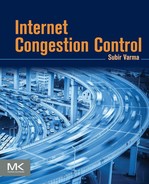
Consider the model shown in Figure 2.1, with a single TCP Reno controlled traffic source passing through a single bottleneck node. Even though this is a very simplified picture of an actual network, Low and Varaiya [8] have shown that there is no loss of generality in replacing all the nodes along the path by a single bottleneck node. Define the following:
W(t): TCP window size in packets at time t
Wf: Window size at which a packet is lost
C: The bottleneck node capacity in packets/sec
B: Buffer count at the bottleneck node in packets
Td: Propagation delay in the forward (or downstream) direction in seconds
Tu: Propagation delay in the backward (or upstream) direction in seconds
T: Total propagation+Transmission delay for a segment
bmax: The maximum buffer occupancy at the bottleneck node in packets
Note that T, which is the fixed part of the round trip latency for a connection, is given by
T=Td+Tu+1C
We first consider the simplest case when the window size is in equilibrium with size Wmax, there is sufficient buffering at the bottleneck node, so no packets get dropped because of overflows, and the link is error free. These assumptions are relaxed in the following sections as the sophistication of the model increases.
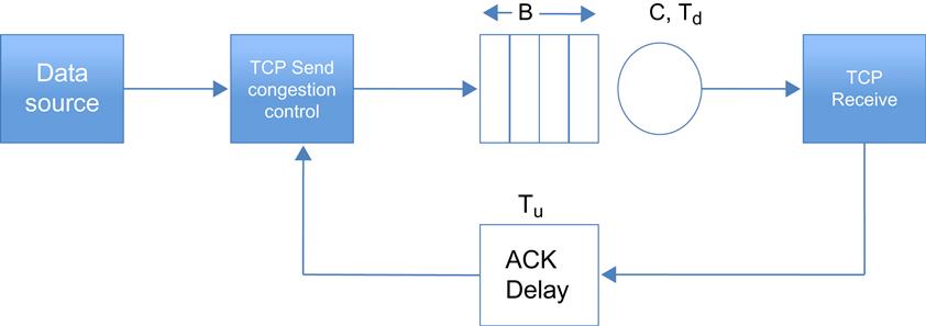
Consider the case when T>Wmax/C, or Wmax/T<C (Figure 2.2). The diagram illustrates the fact that in this case the sender transmits the entire window full of packets before it receives the ACK for first packet back. Hence, the average connection throughput Ravg is limited by the window size and is given by
Ravg=WmaxTwhenWmax<CT (1)
Because the rate at which the bottleneck node is transmitting packets is greater than or equal to the rate at which the source is sending packets into the network, the bottleneck node queue size is zero. Hence, at any instant in time, all the packets are in one of two places: either in the process of being transmitted in the downstream direction (= Ravg.Td packets), or their ACKs are in the process of being transmitted in the upstream direction (= Ravg.Tu ACKs).
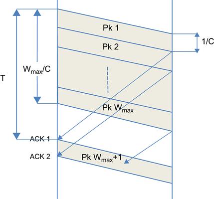
In Figure 2.3, we consider the case when T<Wmax/C, i.e., Wmax/T>C. As the figure illustrates, the ACKs for the first packet in the window arrive at the sender before it has finished transmitting the last packet in that window. As a result, unlike in Figure 2.2, the sender is continuously transmitting. The system throughput is no longer limited by the window size, and is able to attain the full value of the link capacity, that is,
Ravg=CwhenWmax>CT (2)
Combining equations 1 and 2, we get
Ravg=min(WmaxT,C) (3)
In this case, C.Td packets are the process of being transmitted in the downstream direction, and C.Tu ACKs are in the process of being transmitted in the upstream direction, for a total of C.(Td+Tu)=CT packets and ACKs. Because CT<Wmax, this leaves (Wmax−CT) packets from the TCP window unaccounted for, and indeed they are to be found queued up in the bottleneck node! Hence, in equilibrium, the maximum buffer occupancy at the bottleneck node is given by
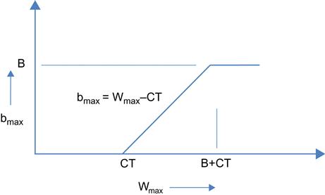
bmax=max(Wmax−CT,0) (4)
Using equations 3 and 4, Ravg can also be written as
Ravg=WmaxT+bmaxC (5)
This shows that the average throughput is given by the window size divided by the total round trip latency, including the queuing delay.
This discussion illustrates the rule of thumb that the optimum maximum window size is given by Wmax=CT, i.e., it should equal the delay-bandwidth product for the connection because at this point the connection achieves its full bandwidth (equal to the link rate). Any increase in Wmax beyond CT increases the length of the bottleneck queue and hence end-to-end delay, without doing anything to increase the throughput.
Figure 2.4 plots Ravg vs Wmax based on equation 3, and as the graph shows, there a knee at Wmax=CT, which is the ideal operating point for the system.
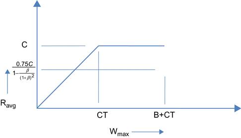
Figure 2.5 plots the maximum buffer occupancy bmax as a function of Wmax based on equation 4. When Wmax increases to B+CT, then bmax=B, and any increase of Wmax beyond this value will cause the buffer to overflow. Note that until this point, we have made no assumptions about the specific rules used to control the window size. Hence, all the formulae in this section apply to any window-based congestion control scheme in the absence of packet drops.
In Section 2.2.2, we continue the analysis for TCP Reno for the case Wmax>B+CT, when packets get dropped because of buffer overflows.
2.2.2 Throughput as a Function of Buffer Size
In Section 2.2.1, we found out that if Wmax>B+CT, then it results in packet drops because of buffer overflows. In the presence of overflows, the variation of the window size W(t) as a function of time is shown in Figure 2.6 for TCP Reno. We made the following assumptions in coming up with this figure:
1. Comparing Figure 2.6 with Figure 1.6 in Chapter 1, we assume that we are in the steady phase of a long file transfer, during which the system spends all its time in the congestion avoidance phase, i.e., the initial Slow-Start phase is ignored, and all packet losses are recovered using duplicates ACKs (i.e., without using timeouts).
2. We also ignore the Fast Recovery phase because it has a negligible effect on the overall throughput, and including it considerably complicates the analysis.
3. Even though the window size W increases and decreases in discrete quantities, we replace it by a continuous variable W(t), thus resulting in what is known as a fluid approximation. This simplifies the analysis of the system considerably while adding only a small error term to the final results.
We now define two additional continuous time variables b(t) and T(t), where b(t) is the fluid approximation to the buffer occupancy process at time t, given by
b(t)=W(t)−CT
and T(t) is the total round trip latency at time t, given by
T(t)=T+b(t)C
The throughput R(t) at time t is defined by
R(t)=W(t)T(t)
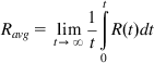
and the average throughput is given by
Ravg=limt→∞1tt∫0R(t)dt
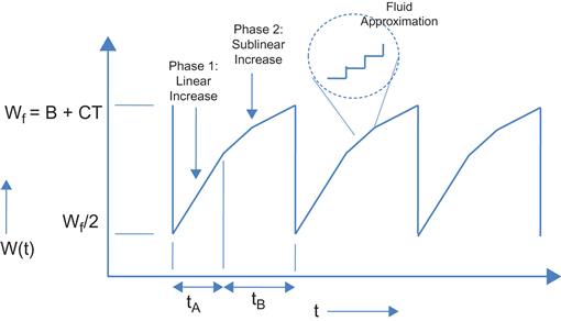
As shown in Figure 2.7, W(t) increases up to a maximum value of Wf=(B+CT) and is accompanied by an increase in buffer size to B, at which point a packet is lost at the bottleneck node because of buffer overflow. TCP Reno then goes into the congestion recovery mode, during which it retransmits the missing packet and then reduces the window size to Wf/2. Using equation 2, if Wf/2 exceeds the delay-bandwidth product for the connection, then Ravg=C. Note that Wf2≥CT![]() implies that
implies that
B+CT2≥CT
which leads to the condition
B≥CT (6)
Hence, if the number of buffers exceeds the delay-bandwidth product of the connection, then the periodic packet loss caused by buffer overflows does not result in a reduction in TCP throughput, which stays at the link capacity C. Combining this with the condition for buffer overflow, we get
Wmax−CT≥B≥CT
as the conditions that cause a buffer overflow but do not result in a reduction in throughput. Equation 6 is a well-known rule of thumb that is used in sizing up buffers in routers and switches. Later in this chapter, we show that equation 6 is also a necessary condition for full link utilization in the presence of multiple connections passing through the link, provided the connections are all synchronized and have the same round trip latency.
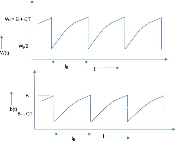
When B<CT, then the reduction in window size to Wf/2 on packet loss leads to the situation where all the packets are either in transmission or being ACK’d, thus emptying the buffer periodically, as a result of which the system throughput falls below C (Figure 2.8). An analysis of this scenario is carried out next.
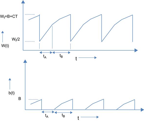
We compute the throughput by obtaining the duration and the number of packets transmitted during each cycle. The increase of the TCP window size happens in two phases, as shown in Figure 2.8:
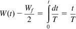
In phase 1, W(t)<CT, which implies that the queue at the bottleneck node is empty during this phase. Hence, the rate at which ACKs are returning to the sender is equal to the TCP throughput R(t)=W(t)/T. This implies that the rate at which the window is increasing is given by
dW(t)dt=dWda⋅dadt=1W(t)⋅W(t)T=1T (7)
where a(t) is the number of ACKs received in time t and da/dt is the rate at which ACKs are being received.
Hence,
W(t)−Wf2=t∫0dtT=tT
This results in a linear increase in the window size during phase 1, as shown in Figure 2.6. This phase ends when W=Wf=CT, so if tA is the duration of this phase, then
CT−Wf2=tAT,
so that
tA=T(CT−Wf2). (8)
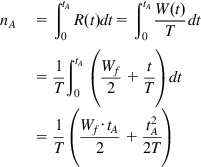
The number of packets nA transmitted during phase 1 is given by
nA=∫tA0R(t)dt=∫tA0W(t)Tdt=1T∫tA0(Wf2+tT)dt=1T(Wf⋅tA2+t2A2T) (9)
 (9)
(9)
In phase 2, W(t)>CT so that the bottleneck node has a persistent backlog. Hence, the rate at which ACKs are returning back to the sender is given by C. It follows that the rate of increase of the window is given by
dW(t)dt=dW(t)da⋅dadt=CW(t) (10)
Hence,
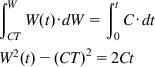
∫WCTW(t)⋅dW=∫t0C⋅dtW2(t)−(CT)2=2Ct
so that
W(t)=√2Ct+(CT)2 (11)
Equation 11 implies that the increase in window size during phase 2 happens in a sublinear fashion, as illustrated in Figure 2.6. During this phase, the window increases until it reaches Wf, and by equation 11, the time required to do this, tB, is given by
tB=W2f−(CT)22C (12)
Because of the persistent backlog at the bottleneck node, the number of packets nB transmitted during phase 2 is given by
nB=CtB=W2f−(CT)22 (13)
The average TCP throughput is given by
Ravg=nA+nBtA+tB (14)
From equations 9 and 13, it follows that
nA+nB=1T(Wf⋅tA2+t2A2T)+W2f−(CT)22
Substituting for tA from equation 8, and after some simplifications, we get
nA+nB=3W2f8 (15)
Thus, the number of packets transmitted during a cycle is proportional to the square of the maximum window size, which is an interesting result in itself and is used several times in Part 2 of this book. Later in this chapter, we will see that this relation continues to hold even for the case when the packet losses are because of random link errors.
Similarly, from equations 8 and 12, we obtain
tA+tB=T(CT−Wf2)+W2f−(CT)22C
which after some simplifications becomes
tA+tB=W2f+(CT)2−CTWf2C (16)
Substituting equations 15 and 16 back into equation 14, we obtain
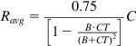
Ravg=34W2fCW2f+(CT)2−CTWf (17)
Note that Wf=B+CT, so that (17) simplifies to
Ravg=0.75[1−B⋅CT(B+CT)2]C (18)
 (18)
(18)
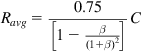
Define β=BCT≤1![]() , so that
, so that
Ravg=0.75[1−β(1+β)2]C (19)
 (19)
(19)
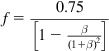
Define f
f=0.75[1−β(1+β)2] (20)
 (20)
(20)
and note that
limβ→0f=0.75andlimβ→1f=1
As shown in Figure 2.9, f monotonically increases from 0.75 to 1 as β![]() increases from 0 to 1, so that Ravg≤C
increases from 0 to 1, so that Ravg≤C![]() .
.
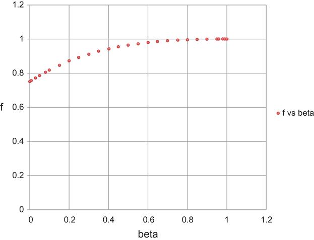
Equations 19 to 21 imply that in a network with a large delay bandwidth product (relative to the buffer size), a TCP Reno–controlled connection is not able to attain its full throughput C. Instead, the throughput maxes out at 0.75C because of the lack of buffering at the bottleneck node. If B exceeds CT, then the throughput converges to C as expected. However, the fact that the throughput is able to get up to 0.75C even for very small buffer sizes is interesting and has been recently used in the design of the CoDel AQM Scheme (see Chapter 4).
2.2.3 Throughput as a Function of Link Error Rate
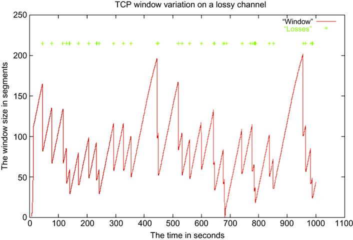
In the presence of random link errors, TCP may no longer be able to attain the maximum window size of B+CT; instead, the window increases to some value that is now a random variable. This is clearly illustrated in Figure 2.10, with the maximum window and consequently the starting window varying randomly. To analyze this case, we have to resort to probabilistic reasoning and find the expected value of the throughput. In Section 2.2.3.1, we consider the case when the lost packets are recovered using the duplicate ACKs mechanism, and in Section 2.2.3.2, we consider the more complex case when packet losses result in timeouts.
To take the random losses into account, we need to introduce a second model in to the system, that of the packet loss process. The simplest case is when packet losses occur independently of one another with a loss probability p; this is the most common loss process used in the literature. Wireless links lead to losses that tend to bunch together because of a phenomenon known as fading. In Section 2.4, we analyze a system in which the packet loss intervals are correlated, which can be used to model such a system.
The type of analysis that is carried out in the next section is known as mean value analysis (MVA) in which we work with the expectations of the random variables. This allows us to obtain closed form expressions for the quantities of interest. There are three other alternative models that have been used to analyze this system:
• Fluid flow models: The fluid flow model that is introduced in Section 2.2.2 can also be extended to analyze the system in the presence of random losses, and this is discussed in Section 2.3.
• Markov chain models [9,10]: These work by defining a state for the system that evolves according to a Markov process, with the state transition probabilities derived as a function of the link error rate. The advantage of this approach is that it is possible to obtain the full distribution of the TCP window size, as opposed to just the mean value. However, it is not possible to get closed form solutions for the Markov chain, which has to be solved numerically.
• Stochastic models [6]: These models replace the simple iid model for packet loss by a more sophisticated stochastic process model. As a result, more realistic packet loss models, such as bursty losses, can also be analyzed. We describe such a model in Section 2.4.
2.2.3.1 Link Errors Recovered by Duplicate ACKs
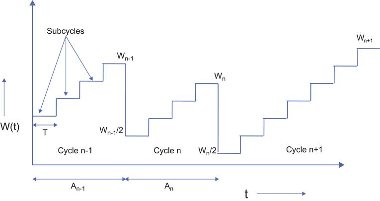
The TCP model used in this section uses discrete states for the window size, as opposed to the fluid model used in Section 2.2.2 [5]. We define a cycle as the time between two loss events (Figure 2.11) and a subcycle as the time required to transmit a single window of packets followed by reception of their ACKs.
In addition to assumptions 1 and 2 from Section 2.2.2, we make the following additional assumptions:
4. All the packets in a window are transmitted back to back at the start of a subcycle, and no other packets are sent until the ACK for the first packet is received, which marks the end of the subcycle and the start of the next one.
5. The time needed to send all the packets in a window is smaller than the round trip time. This assumption is equivalent to stating that the round trip time T(t) is fixed at T(t)=T and equals the length of a subcycle. This is clearly an approximation because we observed in Section 2.2.2 that the T(t) increases linearly after the window size exceeds CT because of queuing at the bottleneck node.
Another consequence of this assumption is that the window increase process stays linear throughout, so we are approximating the sublinear increase for larger window sizes shown in Figure 2.6 (which is caused by the increase in T(t)), by a straight line.
6. Packet losses between cycles are independent, but within a cycle when a packet is lost, then all the remaining packets transmitted until the end of the cycle are also lost. This assumption can be justified on the basis of the back-to-back transmission assumption and the drop-tail behavior of the bottleneck queue.
Wi: TCP window size at the end of the ith cycle
Xi: Number of subcycles in the ith cycle
Yi: Number of packets transmitted in the ith cycle
p: Probability that a packet is lost because of random link error given that it is either the first packet in its round or the preceding packet in its round is not lost.
As shown in Figure 2.11, cycles are indexed using the variable i, and in the ith cycle, the initial TCP window is given by the random variable Wi-1/2, and the final value at the time of packet loss is given by Wi. Within the ith cycle, the sender transmits up to Xi windows of packets, and the time required to transmit a single window of packets is constant and is equal to the duration of the (constant) round trip latency T, so that there are Xi subcycles in the ith cycle. Within each subcycle, the window size increases by one packet as TCP goes through the congestion avoidance phase, so that by the end of the cycle, the window size increases by Xi packets.
We will assume that the system has reached a stationary state, so that the sequences of random variables {Wi}, {Ai}, {Xi} and {Yi} converge in distribution to the random variables W, A, X and Y, respectively. We further define the expected values of these stationary random variables as E(W), E(A), E(X), and E(Y), so that:
E(W): Expected TCP window size at time of packet loss
E(Y): Expected number of packets transmitted during a single cycle
Our objective is to compute Ravg, the average throughput. From the theory of Markov regenerative processes, it follows that
Ravg=E(Y)E(A) (21)
We now proceed to compute E(Y), followed by E(A).
After a packet is lost, Wi–1 additional packets are transmitted before the cycle ends. We will ignore these packets, so that Yi equals the number packets transmitted until the first drop occurs. Under this assumption, the computation of E(Y) is straightforward, given that the number of packets transmitted during a cycle is distributed according to the Bernoulli distribution, that is,
P(Yi=k)=(1−p)k−1p,k=1,2,… (22)
Hence,
E(Y)=1p (23)
Next, note that E(A) is given by
E(A)=E(X)⋅T (24)
where T is the fixed round trip delay for the system. Furthermore, because
Wi=Wi−12+Xi,∀i (25)
it follows by taking expectations on both sides, that the average number of subcycles E(X) is given by
E(X)=E(W)2 (26)
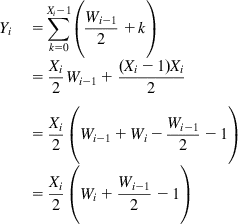
To compute E(W), note that in each subcycle, the TCP window size increases by 1; hence, if we ignore the packets transmitted in the last subcycle, we get
Yi=∑Xi−1k=0(Wi−12+k)=Xi2Wi−1+(Xi−1)Xi2=Xi2(Wi−1+Wi−Wi−12−1)=Xi2(Wi+Wi−12−1) (27)
 (27)
(27)
Assuming that {Xi} and {Wi} are mutually independent sequences of iid random variables and taking the expectation on both sides, we obtain
E(Y)=E(X)2(E(W)+E(W)2−1)=E(X)2(3E(W)2−1) (28)
Substituting the value of E(X) from (27) and using the fact that E(Y)=1/p, we obtain
3(E(W))28−E(W)4−1p=0 (29)
Solving this quadratic equation yields
E(W)=1+√1+24p3packets (30a)
This is approximately equal to
E(W)≈√83ppackets, (30b)
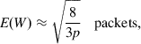 (30b)
(30b)
and from equation 26, we conclude
E(X)≈√23p (31)
 (31)
(31)
Finally, it follows from equations 21, 23, 24, and 31 that
Ravg≈1/pT√2/3p=1T√32ppackets/sec (32)
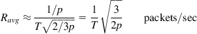 (32)
(32)
Equation 32 is the well-known “square root” law for the expected throughput of a TCP connection in the presence of random link errors that was first derived by Mathis and colleagues [7]. Our derivation is a simplified version of the proof given by Padhye et al. [5]
2.2.3.2 Link Errors Recovered by Duplicate ACKs and Timeouts
In this section, we derive an expression for the average TCP throughput in the presence of duplicate ACK as well as timeouts. As in the previous section, we present a simplified version of the analysis in the paper by Padhye and colleagues [5].
As illustrated in Figure 2.12, we now consider a supercycle that consists of a random number of cycles (recall that cycles terminate with a duplicate ACK–based packet recovery) and a single timeout interval.
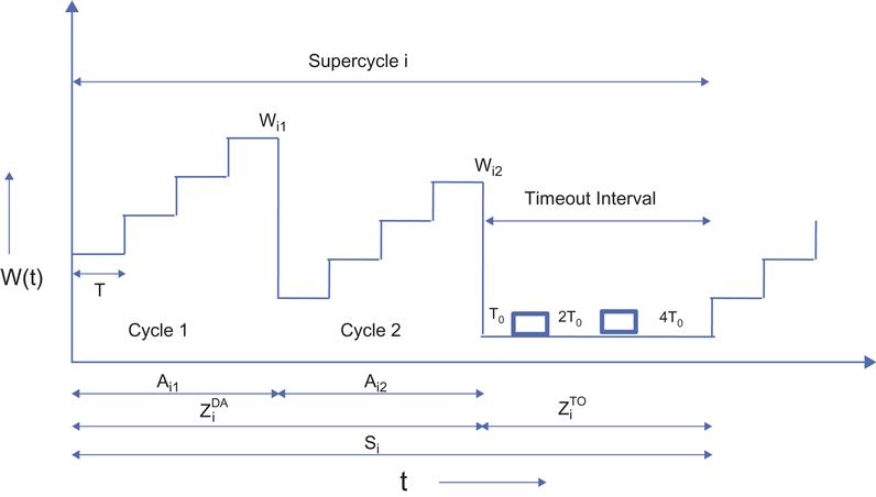
Define the following random variables:
ZDAi![]() : Time duration during which missing packets are recovered using duplicate ACK triggered retransmissions in the ith supercycle. This interval is made of several cycles, as defined in the previous section.
: Time duration during which missing packets are recovered using duplicate ACK triggered retransmissions in the ith supercycle. This interval is made of several cycles, as defined in the previous section.
ni: Number of cycles within a single interval of length ZDAi![]() in the ith supercycle
in the ith supercycle
Yij: Number of packets sent in the jth cycle of the ith supercycle
Xij: Number of subcycles in the jth cycle of the ith supercycle
Aij: Duration of the jth cycle of the ith supercycle
ZTOi![]() : Time duration during which a missing packet is recovered using TCP timeouts
: Time duration during which a missing packet is recovered using TCP timeouts
Mi: Number of packets transmitted in the ith supercycle
Pi: Number of packets transmitted during the timeout interval ZTOi![]()
Si=ZDAi+ZTOi (33)
As in the previous section, we assume that the system is operating in a steady state in which all the random variables defined above have converged in distribution. We will denote the expected value of these random variables with respect to their limit distribution by appending an E before the variable name as before.
Note that the average value of the system throughput Ravg, is given by
Ravg=E(M)E(S) (34)
We now proceed to compute the expected values E(M) and E(S). By their definitions, we have
Mi=∑nij=1Yij+Pi (35)
Si=∑nij=1Aij+ZTOi (36)
Assuming that the sequence {ni} is iid and independent of the sequences {Yij} and {Aij}, it follows that
E(M)=E(n)⋅E(Y)+E(P) (37)
E(S)=E(n)⋅E(A)+E(ZTO) (38)
so that the average throughput is given by
Ravg=E(Y)+E(P)/E(n)E(A)+E(ZTO)/E(n) (39)
Let Q be the probability that the packet loss that ends a cycle results in a timeout, that is, the lost packet cannot be recovered using duplicate ACKs. Then
Pr(n=k)=(1−Q)k−1Q,k=1,2,…
so that
E(n)=1Q (40)
which results in the following expression for Ravg
Ravg=E(Y)+QE(P)E(A)+QE(ZTO) (41)
We derived expressions for E(Y) and E(A) in the last section, namely
E(Y)=1pand (42)
E(A)=T√23p (43)
 (43)
(43)and we now obtain formulae for E(P), E(ZTO) and Q.
1. E(P)
The same packet is transmitted one or more times during the timeout interval ZTO. Hence a sequence of k TOs occurs when there are (k−1) consecutive losses followed by a successful transmission. Hence,
Pr(P=k)=pk−1(1−p),k=1,2,…
from which it follows that
E(P)=11−p. (44)
2. E(ZTO)
Note that the time duration for ZTO with k timeouts are given by
ZTO(k)={(2k−1)T0,fork≤6[63+64(k−6)]T0,fork≥7 (45)
This formula follows from the fact that the value of the timeout is doubled for the first six timer expiries and then kept fixed at 64T0 for further expirations. It follows that
E(ZTO)=∑∞k=1ZTO(k)⋅Pr(P=k)=T01+p+2p2+4p3+8p4+16p5+32p61−p (46)
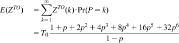 (46)
(46)f(p)=1+p+2p2+4p3+8p4+16p5+32p6 (47)
E(ZTO)=T0f(p)1−p (48)
3. Q
Q is approximated by the formula (see Appendix 2.A for details)
Q=min(1,3E(W))=min(1,3√3p8) (49)
 (49)
(49)
From equations 41 to 44, 48, and 49, it follows that
Ravg=1p+11−pmin(1,3√3p8)T√23p+T0f(p)1−pmin(1,3√3p8) (50)
 (50)
(50)
which after some simplification results in
Ravg=1−p+pmin(1,3√3p8)T(1−p)√23p+T0pf(p)min(1,3√3p8) (51)
 (51)
(51)
For smaller values of p, this can be approximated as
Ravg=1T√23p+T0p(1+32p2)min(1,3√3p8) (52)
 (52)
(52)
This formula was empirically validated by Padhye et al. [5] and was found to give very good agreement with observed values for links in which a significant portion of the packet losses are attributable to timeouts.
2.3 A Fluid Flow Model for Congestion Control
Some of the early analysis work for TCP throughput in the presence of packet drops was done by Floyd [2] and Mathis et al. [7], using a simple heuristic model based on the fluid flow model of the window size evolution (Figure 2.13). This is a simplification of the fluid flow model used in Section 2.2.2 (see Figure 2.6) because the model assumes that the window growth is strictly linear within each cycle.
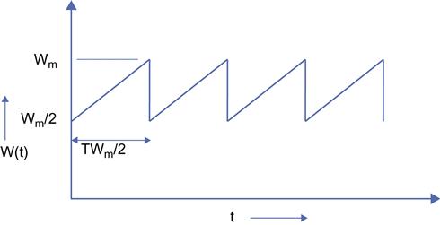
With reference to Figure 2.13, consider a single sample path W(t) of the window size process, such that the value of the maximum window size is Wm, so that the value of the window after a packet loss is Wm/2. During the period in which the window size increases from Wm/2 to Wm (called a cycle), it increases by 1 for every round trip duration T; hence, it takes Wm/2 round trips to increase from Wm/2 to Wm. This implies that the length of a cycle is given by TWm/2 seconds.
Note that the number of packets that are transmitted during a cycle is given by
Y=∫TWm/20R(t)dt
and after substituting R(t)=W(t)/T, we get
Y=TWm/2∫0W(t)Tdt=1T[T(Wm2)2+T2(Wm2)2]=38W2m (53)
 (53)
(53)
It is an interesting coincidence that this formula for the number of packets transmitted in a cycle is identical to the one derived in Section 2.2.2 (see equation 15) because in the earlier case, the derivation took the nonlinear evolution of the window size into account, but in the current case, we made a simplifying linear approximation.
It follows that the throughput for a single cycle of the sample path is given by
R=YTWm/2=34WmT
This expression can also be formulated in terms of Y, as
R=34T√8Y3=1T√3Y2 (54)
Taking the expectations on both sides, it follows that
Ravg=1T√32E(√Y) (55)
The usual way of analyzing this system implicitly makes this assumption that the expectation and the square root operations can be interchanged. Note that this can be done only if Y is a constant, say Y=N, and under this assumption, equation 55 reduces to
Ravg=1T√32√E(Y)=1T√3N2 (56)
Because the system drops one packet of every N that are transmitted, the packet drop rate p is given by p=1/N. Substituting this in equation 56, we obtain
Ravg=1T√32p (57)
 (57)
(57)
and we have recovered the square-root formula. However, this analysis makes it clear that this equation only holds for the case of deterministic number of packets per cycle and is referred to as the “deterministic approximation” in the rest of this book.
If we do not make the deterministic approximation, then for the case when the packet drop variables are iid with probability p, the number of packets per cycle follows the following geometric distribution.
P(Y=n)=(1−p)n−1pn=1,2,…sothat (58)
E(√Y)=∑∞n=1√n(1−p)n−1p (59)
In the absence of a closed form expression for this sum, the final expression for the iid packet loss case is given by
Ravg=1T√3p2∑∞n=1√n(1−p)n−1 (60)
If we approximate the geometric distribution (equation 58) by an exponential distribution with density function given by
fY(y)=λe−λyy≥0 (61)
and to match the two distributions, we set λ=p![]() .
.
Define a random variable X given by
X=√Y
Then it can shown that the density function for X is given by
fX(x)=2λxe−λx2x≥0 (62)
so that
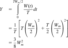
E(X)=2λ∞∫0x2e−λx2dx=2λlimx→∞[√π4λ3/2erf(√λx)−xe−λx22λ]=limx→∞[12√πλerf(√λx)−xe−λx2]=12√πλ (63)
 (63)
(63)
where erf is the standard error function. From equations 55 and 63, it follows that
Ravg=1T√3π8p (64)
 (64)
(64)
where we substituted p back into the equation. Hence, we have succeeded in recovering the square-root formula using the more exact calculation. The constant in equation 64 computes to 1.08, as opposed to 1.22 in equation 57, so it results in a slightly lower average throughput.
In the calculation done in Section 2.2.3.1, the assumption following equation 28 that the {Xi} and {Wi} sequences are independent also results in implicitly introducing the deterministic assumption into the computation, so that the final result coincides with that of the deterministic case.
As we will see later in Part 2, the most important information in the formula for the average throughput is not the constant but the nature of the functional dependence on p and T. Because the deterministic approximation gives the correct functional dependence while using fairly straightforward computations, we will follow the rest of the research community in relying on this technique in the rest of this book.
Equation 53 can be used to derive an expression of the distribution of the maximum TCP window size Wm, and this is done next. Because Wm=√8Y3![]() , it follows that
, it follows that
P(Wm≤x)=P(Y≤3x28)
Again, using the exponential distribution (equation 61) for the number of packets per cycle, it follows that
P(Wm≤x)=1−e−3px28
so that the density function for Wm is given by
fWm(x)=3px4e−3px28x≥0.
A General Procedure for Computing the Average Throughput
Basing on the deterministic approximation, we provide a procedure for computing the average throughput for a congestion control algorithm with window increase function given by W(t) and maximum window size Wm. This procedure is used in the next section as well as several times in Part 2 of this book:
1. Compute the number of packets Y transmitted per cycle by the formula
Yα(Wm)=1T∫T0W(t,α)dt
In this equation, T is the round trip latency, and α![]() represents other parameters that govern the window size evolution.
represents other parameters that govern the window size evolution.
2. Equate the packet drop rate p to Y, using the formula
Yα(Wm)=1p
If this equation can be inverted, then it leads to a formula for Wm as a function of p, that is,
Wm=Y−1α(1p)
3. Compute the cycle duration τ(Wm)![]() for a cycle as a function of the maximum window size.
for a cycle as a function of the maximum window size.
4. The average throughput is then given by
Ravg=1/pτ(Wm)=1/pτ(Y−1α(1p))
The formula for the window increase function W(t,α)![]() can usually be derived from the window increase-decrease rules. Note that there are algorithms in which the inversion in step 2 is not feasible, in which case we will have to resort to approximations. There are several examples of this in Chapter 5.
can usually be derived from the window increase-decrease rules. Note that there are algorithms in which the inversion in step 2 is not feasible, in which case we will have to resort to approximations. There are several examples of this in Chapter 5.
2.3.1 Throughput for General Additive Increase/Multiplicative Decrease (AIMD) Congestion Control
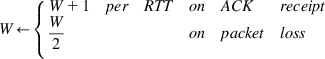
Recall that the window increase–decrease rules for TCP Reno can be written as:
W←{W+1perRTTonACKreceiptW2onpacketloss (65)
 (65)
(65)This rule can be generalized so that the window size increases by a packets per RTT in the absence of loss, and it is reduced by a fraction bW on loss. This results in the following rules:
W←{W+aperRTTonACKreceipt(1−b)Wonpacketloss (66)
This is referred to as an AIMD congestion control [11], and has proven to be very useful in exploring new algorithms; indeed, most of the algorithms in this book fall within this framework. In general, some of the most effective algorithms combine AIMD with increase decrease parameters (a,b) that are allowed to vary as a function of either the congestion feedback or the window size itself. Here are some examples from later chapters:
• By choosing the value of a, the designer can make the congestion control more aggressive (if a>1) or less aggressive (if a<1) than TCP Reno. The choice a>1 is used in high-speed networks because it causes the window to increase faster to take advantage of the available bandwidth. Protocols such as High Speed TCP (HSTCP), TCP BIC, TCP FAST and TCP LEDBAT use an adaptive scheme in which they vary the value of a depending on the current window size, the congestion feedback, or both.
• The value of b influences how readily the connection gives up its bandwidth during congestion. TCP Reno uses a rather aggressive reduction of window size by half, which causes problems in higher speed links. By choosing b<0.5, the reduction in window size is smaller on each loss, which leads to a more stable congestion control algorithm. But this can lead to fairness issues because existing connections don’t give up their bandwidth as readily. Protocols such as Westwood, Data Center TCP (DCTCP) and HSTCP vary b as a function of the congestion feedback (Westwood, DCTCP) or the window size (HSTCP).
Using the deterministic approximation technique from the previous section, we derive an expression for the throughput of AIMD congestion control.
With reference to Figure 2.14, the TCP window size reduces from Wm to (1-b)Wm on packet loss (i.e., a reduction of bWm packets). On each round trip, the window size increases by a packets, so that it takes bWm/a round trips for the window to get back to Wm. This implies that the length of a cycle is given by
τ=TWmbaseconds.
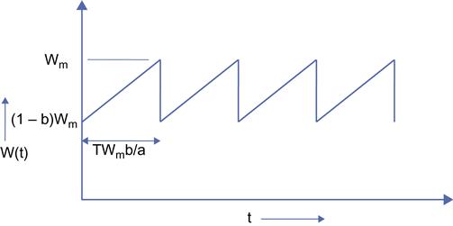
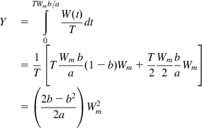
The average number of packets transmitted over a single cycle is then given by:
Y=TWmb/a∫0W(t)Tdt=1T[TWmba(1−b)Wm+T2Wm2baWm]=(2b−b22a)W2m (67)
 (67)
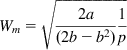
(67)By step 2 of the deterministic approximation procedure, equating Y to 1/p leads to
1p=(2b−b22a)W2m
so that
Wm=√2a(2b−b2)1p (68)
 (68)
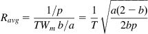
(68)The average response time Ravg is then given by
Ravg=1/pTWmb/a=1T√a(2−b)2bp (69)
 (69)
(69)Comparing equation 69 with the equivalent formula for TCP Reno (equation 57), it follows that an AIMD congestion control algorithm with parameters (a,b) has the same average throughput performance as TCP Reno if the following equation is satisfied:
a=3b2−b. (70)
In Chapter 3, we generalize the notion of AIMD congestion control by introducing nonlinearities in the window increase–decrease rules, which is called generalized AIMD or GAIMD congestion control. Note that equation 69 holds only for the case when the parameters a and b are constants. If either of them is a function of the congestion feedback or the current window size, it leads to a nonlinear evolution of the window size for which this analysis does not hold.
2.3.2 Differentiating Buffer Overflows from Link Errors
The theory developed in Sections 2.2 and 2.3 can be used to derive a useful criterion to ascertain whether the packet drops on a TCP connection are being caused because of buffer overflows or because of link errors.
When buffer overflows are solely responsible for packet drops, then N packets are transmitted per window cycle, where N is given by equation 15
N=3W2f8.
Because one packet is dropped per cycle, it follows that packet drop rate is given by
p=1N=83W2f. (71)
Because Wf≈CT![]() (ignoring the contribution of the buffer size to Wf), it follows that
(ignoring the contribution of the buffer size to Wf), it follows that
p(CT)2≈83 (72)
when buffer overflows account for most packet drops.
On the other hand, when link errors are the predominant cause of packet drops, then the maximum window size Wm achieved during a cycle may be much smaller than Wf. It follows that with high link error rate,
W2m≪W2f
so that by equation 53,
p=1E(Y)=83E(W2m)≫83W2f.
It follows that if
p(CT)2≫83 (73)
then link errors are the predominant cause of packet drops. This criterion was first proposed by Lakshman and Madhow [4] and serves as a useful test for the prevalence of link errors on a connection with known values for p, C, and T.
2.4 A Stochastic Model for Congestion Control
In this section, following Altman and colleagues [6], we replace the simple packet loss model that we have been using with a more sophisticated loss model with correlations among interloss intervals.
Define the following model for the packet loss process:
{τn}+∞n=−∞![]() : Sequence of time instants at which packets are lost
: Sequence of time instants at which packets are lost
Sn=τn+1−τn![]() : Sequence of intervals between loss instants
: Sequence of intervals between loss instants
d=E(Sn)![]() : The average interloss interval
: The average interloss interval
U(k)=E[SnSn+k]![]() : The correlation function for the interloss interval process.
: The correlation function for the interloss interval process.
Rn![]() : Value of the TCP throughput just before nth packet loss at Tn
: Value of the TCP throughput just before nth packet loss at Tn
Recall that the throughput at time t is given by
R(t)=W(t)TsothatdRdt=1TdWdt (74)
For TCP Reno, dW/dt=1/T under the assumption that the round trip delay remains constant during a cycle, so that
dRdt=1T2 (75)
so that R(t) increases linearly with slope 1/T2. From equation 75, it follows that
Rn+1=(1−b)Rn+SnT2 (76)
where (1–b) is the window decrease factor on packet loss (i.e., we are using the AIMD window rules in equation 66 with b<1 and a=1).
Equation 76 is a stochastic linear differential equation, with a solution given by Brandt [12].
R*n=1T2∑∞k=0(1−b)kSn−1−k (77)
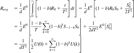
To compute the average throughput Ravg, we start with its definition given by
Ravg=limt→∞1t∫t0R(t)dt
Using the inversion formula from Palm calculus [13] and substituting from equations 76 and 77, it follows that
Ravg=1dE0⌊τ1∫0[(1−b)R0+tT2]dt⌋=1dE0[(1−b)R0S0+S202T2]=1dE0⌊1−bT∑∞k=0(1−b)kS−1−kS0⌋+12dT2E0[S20]=1dT2⌊12U(0)+∑∞k=1(1−b)kU(k)⌋ (78)
 (78)
(78)
Note that in this formula, we have used the fact that τ0=0![]() so that S0=τ1
so that S0=τ1![]() . The expectation E0 is with respect to the Palm measure P0 that is conditioned on sample paths for which τ0=0
. The expectation E0 is with respect to the Palm measure P0 that is conditioned on sample paths for which τ0=0![]() .
.
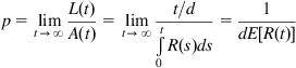
To express this formula as a function of the packet loss probability p, note that if A(t) is the number of packets transmitted and L(t) is the number of loss events until time t, then
p=limt→∞L(t)A(t)=limt→∞t/dt∫0R(s)ds=1dE[R(t)] (79)
 (79)
(79)
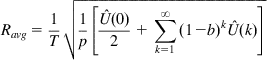
Define the normalized correlation function as
ˆU(k)=U(k)d2
Substituting the value of d from (79) into (78), it follows that
Ravg=1T√1p[ˆU(0)2+∑∞k=1(1−b)kˆU(k)] (80)
 (80)
(80)
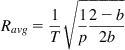
For the case of deterministic interpacket loss intervals, it follows that
ˆU(k)=1k=0,1,2,…
so that
Ravg=1T√1p2−b2b (81)
 (81)
(81)
which coincides with equation 72 in the previous section. Substituting b=½, we again recover the square-root formula.
Equation 80 implies that a correlation between packet loss intervals leads to an increase in the average throughput.
2.5 Why Does the Square-Root Formula Work Well?
From equation 80 in the previous section, it follows that increasing the variance or the presence of correlation between the interpacket loss intervals increases the average throughput. Because in practice, interpacket loss intervals have a finite variance and probably are correlated as well, it begs the question of why equation 60 work so well in practice even though it was derived under the assumption of deterministic interloss intervals.
Recall that we made the assumption in Section 2.2.3.1 that the rate of increase of the congestion window is linear, as shown in the dashed curve in Figure 2.15. This is equivalent to assuming that the round trip latency remains constant over the course of the window increase. This is clearly not the case in reality because the latency increases with increasing window size attributable to increasing congestion in the network. Hence, the actual increase in window size becomes sublinear as shown in the solid curve in Figure 2.15; indeed, we analyzed this model in Section 2.2.2.
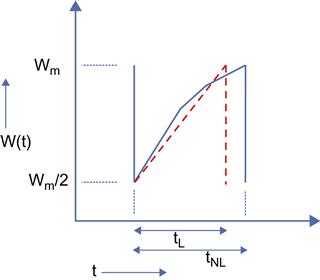
We will assume that the bottleneck node for both cases has the same buffer size, so that both of these windows increase to the same value Wm at the end of their cycles. Let RL be the throughput of the linear model and let RNL be the throughput of the nonlinear model. It follows that
RL=NLtLandRNL=NNLtNL
where NL is the number of packets transmitted in the linear model and NNL is the number for the nonlinear model. In equations 15 and 53, we computed NNL and NL, respectively, and it turns out that NNL=NL. However because tL<tNL, it follows that RL> RNL. Hence, the reason why the linear model with deterministic number of packets per cycle works well is because of the cancellation of the following two error sources:
2.6 The Case of Multiple Parallel TCP Connections
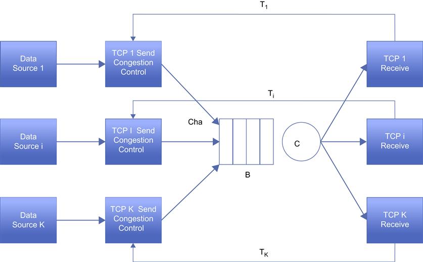
In this section, following Bonald [14], we extend the analysis in Section 2.2 to the case when there are multiple TCP connections passing through a single bottleneck node (Figure 2.16). We will consider two cases:
• In Section 2.6.1, we discuss the homogeneous case when all connections have the same round trip latency.
• In Section 2.6.2, we discuss the heterogeneous case in which the round trip latencies are different.
In general, the presence of multiple connections increases the complexity of the model considerably, and in most cases, we will have to resort to approximate solutions after making simplifying assumptions. However, this exercise is well worth the effort because it provides several new insights in the way TCP functions in real-world environments. The analysis in this section assumes that there are no packet drops due to link errors so that all losses are attributable to buffer overflows.
Consider the following system: There are K TCP connections passing through the bottleneck link.
Wi(t) TCP window size for the ith session, i=1,2,…,K
W(t)=W1(t)+W2(t)+…+WK(t) The total window size attributable to all the K sessions.
Tdi![]() : Propagation delay in the forward (or downstream) direction in seconds for the ith session, i=1,2,…,K
: Propagation delay in the forward (or downstream) direction in seconds for the ith session, i=1,2,…,K
Tui![]() : Propagation delay in the backward (or upstream) direction in seconds for the ith session, i=1,2,…,K
: Propagation delay in the backward (or upstream) direction in seconds for the ith session, i=1,2,…,K
Ti: Total propagation+Transmission delay for a segment, i=1,2,…,K
Ri(t), Ravgi![]() : Instantaneous throughput and the average throughput of the ith session, i=1,2,…,K
: Instantaneous throughput and the average throughput of the ith session, i=1,2,…,K
R(t), Ravg: Instantaneous total throughput and average total throughput attributable to all the K sessions.
The constants Wmax, C, and B and the variable b(t) are defined as in Section 2.2.1.
2.6.1 Homogeneous Case
We will initially consider the homogeneous case in which the propagation+transmission delays for all the sessions are equal (i.e., T=Ti=Tj, i, j=1, 2,…,K).
The basic assumption that is used to simplify the analysis of this model is that of session synchronization. This means that the window size variations for all the K sessions happen together (i.e., their cycles start and end at the same time). This assumption is justified from observations made by Shenker et al. [3] in which they observed that tail drop causes the packet loss to get synchronized across all sessions. This is because packets get dropped because of buffer overflow at the bottleneck node; hence, because typically multiple sessions encounter the buffer overflow condition at the same time, their window size evolution tends to get synchronized. This also results in a bursty packet loss pattern in which up to K packets are dropped when the buffer reaches capacity. This implies that
dWi(t)dt=dWj(t)dt∀i,j (82)
because the rate at which a window increases is determined by the (equal) round trp latencies. From the definition of W(t) and equations 7 and 82, it follows that
dW(t)dt=KTwhenW(t)≤CT (83)
From equations 10 and 82, we obtain
dW(t)dt=KCW(t)whenW(t)>CT (84)
Note that
Ri(t)=R(t)Ki=1,2,…,K (85)
so that it is sufficient to find an expression for total throughput R(t).
As in Section 2.2.2, the time evolution of the total window W(t) shows the characteristic sawtooth pattern, with the sum of the window sizes W(t) increasing until it reaches the value Wf=B+CT. This results in synchronized packet losses at all the K connections and causes W(t) to decrease by half to Wf/2. When this happens, there are two cases:
1. Wf/2>CT (i.e., B>CT)
This condition holds for a network with a small delay-bandwidth product. In this case, the bottleneck queue is always occupied, hence
R(t)=CandRi(t)=CKi=1,2,…,K (86)
2. Wf/2<CT (i.e., B<CT)
This condition holds for a network with a large delay-bandwidth product. In this case, there are two phases with W(t)<CT in phase 1 and W(t)>CT in phase 2. The calculations are exactly the same as in Section 2.2.2, and they lead to the following formula for the average total throughput Ravg
Ravg=0.75[1−β(1+β)2]C,whereβ=BCT (87)
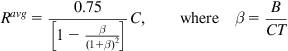 (87)
(87)
which leads to
Ravgi=0.75[1−β(1+β)2]CKi=1,2,…,K (88)
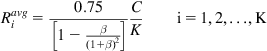 (88)
(88)
Note that the total throughput Ravg is independent of the number of connections K. Equation 87 also implies that as a result of the lack of buffers in the system and the synchronization of the TCP sessions, the link does not get fully used even with a large number of sessions. Case 1 also leads to the interesting result that for the fully synchronized case, the amount of buffering required to keep the link continuously occupied is given by CT and is independent of the number of connections passing through the link.
2.6.2 Heterogeneous Case
In this case, the session propagation delays Ti, i=1,2,…,K may be different.
Recall that the throughput Ri(t) for session i is defined by the formula
Ri(t)=Wi(t)Ti+b(t)Ci=1,2,…,K (89)
Hence, for the case when the bottleneck link is fully used, we have
∑Ki=1Ri(t)=C,
so that
∑Ki=1Wi(t)b(t)+CTi=1 (90)
The following equation follows by reasoning similar to that used to derive equation 7.
dWi(t)dt=1Ti+b(t)Ci=1,2,…,K (91)
Following the analysis in Section 2.2.2, the average throughput for the ith session is given by
Ravgi=38(Wfi)2tAi+tBii=1,2,…,K (92)
where, as before, tAi![]() is the average time interval after a packet loss when the buffer is empty, and tBi
is the average time interval after a packet loss when the buffer is empty, and tBi![]() is the average time interval required for the buffer to fill up.
is the average time interval required for the buffer to fill up.
In general, it is difficult to find closed form solutions for Wi(t) and an expression for Wfi![]() from these equations, even if synchronization among sessions is assumed. Hence, following Bonald [14], we do an asymptotic analysis, which provides some good insights into the problem.
from these equations, even if synchronization among sessions is assumed. Hence, following Bonald [14], we do an asymptotic analysis, which provides some good insights into the problem.
1. The case of large buffers
Define βi=BCTi![]() , i=1,2,…,K and assume that βi
, i=1,2,…,K and assume that βi![]() is very large, that is, the delay bandwidth product for all sessions is negligible compared with the number of buffers in the bottleneck node. This means that the bottleneck buffer is continuously occupied, so that tAi=0
is very large, that is, the delay bandwidth product for all sessions is negligible compared with the number of buffers in the bottleneck node. This means that the bottleneck buffer is continuously occupied, so that tAi=0![]() . Using equation 91, this leads to
. Using equation 91, this leads to
dWi(t)dt≈Cb(t),i=1,2,…,K (93)
Equation 93 implies that all the K windows increase at the same rate; hence, the maximum window sizes are also approximately equal, so that Wfi≈Wfj![]() , and tBi≈tBj
, and tBi≈tBj![]() for all i,j. From equation 92, it then follows that
for all i,j. From equation 92, it then follows that
Ravgi≈Ravgji,j=1,2,…,K (94)
Hence, when the number of buffers in the bottleneck node is large, each connection gets a fair share of the capacity despite any differences in propagation delays.
2. The case of large delay-bandwidth product
We assume that βi![]() , i=1,2,…,K is very small, that is, the delay-bandwidth product for each session is very large compared with the number of buffers in the bottleneck node. We also make the assumption that the K connections are synchronized, so that they drop their packets at the bottleneck node at the same time.
, i=1,2,…,K is very small, that is, the delay-bandwidth product for each session is very large compared with the number of buffers in the bottleneck node. We also make the assumption that the K connections are synchronized, so that they drop their packets at the bottleneck node at the same time.
From equation 91, it follows that
dWi(t)dt≈1Ti
so that
Wi(t)Wj(t)≈TjTii,j=1,2,…,K (95)
and from equations 63 and 69, it follows that
Ri(t)Rj(t)≈Wi/TiWj/Tj≈(TjTi)2i,j=1,2,…,K (96)
Hence, for large delay-bandwidth products, TCP Reno with tail drop has a very significant bias against connections with larger propagation delays. At first glance, it may seem that equation 96 contradicts the formula for the average throughput (60) because the latter shows only an inverse relationship with the round trip latency T. However, note that by making the assumption that the K sessions are synchronized, their packet drop probabilities p become a function of T as well, as shown next. We have
RiavgRjavg=TjTi√pjpiand furthermore (97)
pi≈1E(Wi)(t/Ti) (98)
where t is common cycle time for all the K connections and E(Wi)t/Ti is expected number of packets transmitted per cycle. Substituting E(Wi)=√83p![]() from equation 30b, it follows that pi=38(Tit)2
from equation 30b, it follows that pi=38(Tit)2![]() . Substituting this expression into equation 97, we obtain
. Substituting this expression into equation 97, we obtain
RiavgRjavg=(TjTi)2. (99)
Using heuristic agreements, equation 99 can be extended to the case when the average throughput is given by the formula:
Ravg=hTepd (100)
where h, e, and d are constants. Equations such as equation 100 for the average throughput arise commonly when we analyze congestion control algorithms in which the window increase is no longer linear (see Chapter 5 for several examples of this). For example, for TCP CUBIC, e=0.25, and d=0.75.
It can be shown that the throughput ratio between synchronized connections with differing round trip latencies is given by
RiavgRjavg=(TjTi)e1−d (101)
To prove equation 101, we start with equation 100 so that
RiavgRjavg=(TjTi)e(pjpi)d (102)
Because the probability of a packet loss is the inverse of the number of packets transmitted during a cycle and t/Ti is the number of round trips in t seconds, it follows that
pi=1E(Wi)(t/Ti)=Teipdth (103)
where we have used the formula
E(W)=RavgT=hTe−1pd
From equation 103, it follows that
pi=(Teith′)1/1−d (104)
Substituting equation 104 into equation 102 leads to equation 101. This equation was earlier derived by Xu et al. [15] for the special case when e=1. It has proven to be very useful in analyzing the intraprotocol fairness properties of congestion protocols, as shown in Chapter 5.
Equation 101 is critically dependent on the assumption that the packet drops are synchronized among all connections, which is true for tail-drop queues. A buffer management policy that breaks this synchronization leads to a fairer sharing of capacity among connections with unequal latencies. One of the objectives of RED buffer management was to break the synchronization in packet drops by randomizing individual packet drop decisions. Simulations have shown that RED indeed achieves this objective, and as a result, the ratio of the throughputs of TCP connections using RED varies as the first power of their round trip latencies rather than the square.
2.7 Further Reading
TCP can also be analyzed by embedding a Markov chain at various points in the window size evolution and by using the packet loss probability to control the state transitions. The stationary distribution of the window size can then be obtained by numerically solving the resulting equations. This program has been carried out by Casetti and Meo [9], Hasegawa and Murata [16], and Kumar [10]. Because this technique does not result in closed form expressions, the impact of various parameters on the performance measure of interest are not explicitly laid out.
Tinnakornsrisuphap and Makowski [17] carry out an analysis of the congestion control system with multiple connections and RED by setting up a discrete time recursion equation between quantities of interest and then show that by using limit theorems the equations converge to a simpler more robust form. Budhiraja et al. [18] analyze the system by directly solving a stochastic differential equation for the window size and thereby derive the distribution of the window size in steady state.
Appendix 2.A Derivation of Q=min(1,3/E(W))
Recall that Q is the probability that a packet loss that ends a cycle results in a timeout. Note that the timeout happens in the last cycle of the supercycle (see Figure 2.9). We will focus on the last subcycle of the last cycle, which ends in a timeout, as well as the subcycle just before it, which will be referred to as the “penultimate” subcycle.
Let w be the window size during the penultimate subcycle and assume that packets f1,…,fw are transmitted during the penultimate subcycle. Of these packets, f1,…,fk are ACKed, and the remaining packets fk+1,…,fw are dropped (using assumption 6). Because f1,…,fk are ACKed, this will result in the transmission of k packets in the last subcycle, say s1,…,sk. Assume that packet sm+1 is dropped in the last round; this will result in the dropping of packets sm+2,…,sk. Note that packets s1,…,sm that are successfully transmitted in the last round will result in the reception of m duplicate ACKs at the sender. Hence, a TCP timeout will result if m=0,1, or 2 because in this case, there are not enough ACKs received to trigger a duplicate ACK–based retransmission.
A(w,k): The probability that the first k packets are ACK’d in a subcycle of w packets given that there is a loss of one or more packets during the subcycle
D(n,m): The probability that m packets are ACK’d in sequence in the last subcycle (where n packets are sent) and the rest of the packets in the round, if any, are lost.
ˆQ(w)![]() : The probability that a packet loss in a penultimate subcycle with window size w results in a timeout in the last subcycle.
: The probability that a packet loss in a penultimate subcycle with window size w results in a timeout in the last subcycle.
Then
A(w,k)=(1−p)kp1−(1−p)w (A1)
D(n,m)={(1−p)mpifm≤n−1(1−p)nifm=n (A2)
From the discussion above, the last subcycle will result in a timeout if (1) the window size in the penultimate subcycle is 3 or less; (2) if the window size in the penultimate round is greater than 3 but only two or fewer packets are transmitted successfully; or (3) if the window size in the penultimate round is greater than 3 and the number of packets that are successfully transmitted is 3 or greater but only 0, 1, or 2 of the packets in the last round are transmitted successfully.
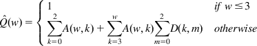
In all the three cases above, not enough duplicate ACKs are generated in the last subcycle to trigger a retransmission. It follows that ˆQ(w)![]() is given by
is given by
ˆQ(w)={1ifw≤3∑2k=0A(w,k)+∑wk=3A(w,k)∑2m=0D(k,m)otherwise (A3)
 (A3)
(A3)
Substituting equations A1 and A2 into equation A3, it follows that
ˆQ(w)=min(1,(1−(1−p)3)(1+(1−p)3(1−(1−p)w−3))1−(1−p)w) (A4)
Using L’Hopital’s rule, it follows that
limp→0ˆQ(w)=3w
A very good approximation to Q(w) is given by
ˆQ(w)≈min(1,3w) (A5)
Note that
Q=∑∞w=1Q(w)P(W=w)=E[ˆQ]
Making the approximation
Q≈ˆQ(E(W))
we finally obtain
Q≈min(1,3E(W)). (A6)