Flow Control for Video Applications
This chapter discusses congestion control for video streaming applications. With the explosion in video streaming traffic in recent years, there arose a need to protect the network from congestion from these types of sources and at the same time ensure good video performance at the client end. The industry has settled on the use of TCP for transmitting video even though at first cut, it seems to be an unlikely match for video’s real-time needs. This problem was solved by a combination of large receive playout buffers that can smoothen out the fluctuations caused by TCP rate control and an ingenious algorithm called HTTP Adaptive Streaming (HAS) or Dynamic Adaptive Streaming over HTTP (DASH). HAS runs at the client end and controls the rate at which “chunks” of video data are sent from the server, such that the sending rate closely matches the rate at which the video is being consumed by the decoder. This chapter describes the work in this area, including several ingenious HAS algorithms for controlling the video transmission rate.
Keywords
video congestion control; video streaming over TCP; HTTP Adaptive Streaming; HAS; Dynamic Adaptive Streaming over HTTP; DASH; Adaptive Bit Rate; ABR; Microsoft HTTP Smooth Streaming; HSS; Apple HTTP Live Streaming; HLS; Adobe HTTP Dynamic Streaming; HDS; Netflix Adaptive Streaming; FESTIVE video congestion control; video congestion control using model predictive control; PANDA video congestion control
6.1 Introduction
Video streaming has grown in popularity as the Internet matures and currently consumes more bandwidth than any other application. Most of this traffic is driven by consumer consumption of video, with services such as Netflix and YouTube leading the pack. Video traffic comes in two flavors, video on demand (VoD) and live-video streaming. VoD traffic is from stored media and is streamed from servers, and it constitutes the majority of the video traffic.
Video has some fundamental differences in transmission requirements compared with traditional data traffic, such as the fact that there are real-time constraints in the delivery of video traffic to the client player. As explained in Section 6.2, this constraint arises because the client video device expects data to be constantly available so that it can keep updating the screen at a constant rate (which is usually 30 frames/s). If there is a hiccup in this process and no data is available, then this results in a temporarily frozen screen while the network catches up.
Most of the early work on packet video transmission focused on providing real-time transmission by means of new techniques that supported resource reservations and QoS (quality of service) provisioning in the network. In the Internet Engineering Task Force (IETF), protocols such as RSVP and IntServ were designed during the 1990s with the intent of using them for provisioning network resources for streaming video delivery. Other protocols that were designed during this era to support real-time streaming included RTP (Real Time Protocol), which served as the packet transport; RTSP (Real Time Streaming Protocol); and RTCP (Real Time Control Protocol), which were used to configure and control the end systems to support the video streams. Even though these protocols are now widely used for supporting real-time video in the Internet, most operators balked at supporting these protocols for consumer video transmission because of the extra complexity and cost involved at both the servers and in the network infrastructure.
During the early years of the Web, the conventional wisdom was that video streaming would have to be done over the User Datagram Protocol (UDP) because video did not require the absolute reliability that TCP provided, and furthermore, TCP retransmissions are not compatible with real-time delivery that video requires. In addition, it was thought that the wide rate variations that are a result of TCP’s congestion control algorithm would be too extreme to support video streams whose packet rate is steady and does not vary much. Because of UDP does not come with any congestion control algorithm, there was considerable effort expended in adding this capability to UDP so it could use it for carrying video streams and at the same time coexist with regular TCP traffic. The most significant result from this work was a congestion control algorithm called TCP Friendly Congestion Control (TFRC) [1]. This was a rate-based algorithm whose design was based on the square-root formula for TCP throughput derived in Chapter 2. The sender kept estimates of the round trip latency and Packet Drop Rate and then used the square root formula to estimate the throughput that a TCP connection would experience under the same conditions. This estimate was then used to control the rate at which the UDP packets were being transmitted into the network.
The video transmission landscape began to change in the early 2000s when researchers realized that perhaps TCP, rather than UDP, could also be used to transmit video. TCP’s rate fluctuations, which were thought to be bad for video, could be overcome by using a large receive buffer to dampen them out. Also because most video transmissions were happening over the Web, using the HyperText Transfer Protocol (HTTP) for video was also very convenient. The combination of HTTP/TCP for video delivery had several benefits, including:
• TCP and HTTP are ubiquitous, and most video is accessed over the Web.
• A video server built on top of TCP/HTTP uses commodity HTTP servers and requires no special (and expensive) hardware or software pieces.
• HTTP has built-in Network Address Translation (NAT) traversal capabilities, which provide more ubiquitous reach.
• The use of HTTP means that caches can be used to improve performance. A client can keep playback state and download video segments independently from multiple servers while the servers remain stateless.
• The use of TCP congestion control guarantees that the network will remain stable in the presence of high–bit rate video streams.
The initial implementations of video over HTTP/TCP used a technique called Progressive Download (PD), which basically meant that the entire video file was downloaded as fast as the TCP would allow it into the receiver’s buffer. Furthermore, the client video player would start to play the video before the download was complete. This technique was used by YouTube, and even today YouTube uses an improved version of the PD algorithm called Progressive Download with Byte Ranges (PD-BR). This algorithm allows the receiver to request specific byte ranges of the video file from the server, as opposed to the entire file.
A fundamental improvement in HTTP/TCP delivery of video was made in the mid 2000s with the invention of an algorithm called HTTP Adaptive Streaming (HAS), which is also sometimes known by the acronym DASH (Dynamic Adaptive Streaming over HTTP). This algorithm is described in detail in Section 6.3 and was first deployed by Move Networks and then rapidly after that by the other major video providers. Using HAS, the video receiver is able to adaptively change the video rate so that it matches the bandwidth that the network can currently support. From this description, HAS can be considered to be a flow control rather than a congestion control algorithm because its objective is to keep the video receive buffer from getting depleted rather than to keep network queues from getting congested. In this sense, HAS is similar to TCP receive flow control except for the fact that the objective of the latter algorithm is to keep the receive buffer from overflowing. HAS operates on top of TCP congestion control, albeit over longer time scales, and the interaction between the two is rich source of research problems.
HAS remains an area of active research, and the important issues such as the best algorithm to control the video bit rate, the interaction of HAS with TCP, and the interaction of multiple HAS streams at a bottleneck node are still being investigated. There have been several suggestions to improve the original HAS bit rate adaptation algorithm, some of which are covered in Section 6.3.
Today the reliable delivery of even high-quality high-definition (HD) video has become commonplace over the Web, and some of the credit for this achievement can be attributed to the work described in this chapter.
The rest of this chapter is organized as follows: Section 6.2 introduces the fundamentals of video delivery over packet networks, Section 6.3 describes the HAS protocol, Section 6.4 introduces Adaptive Bit Rate (ABR) algorithms, Section 6.5 describes several ABR algorithms that have been proposed in the literature, and Sections 6.6 and 6.7 discuss the TCP throughput measurement problem and the interaction between TCP and ABR.
An initial reading of this chapter can be done in the sequence 6.1→6.2→6.3→6.4→6.5 followed by either 6.5.1 or 6.5.2 or 6.5.3 (depending on the particular type of ABR algorithm the reader is interested in). Section 6.6 and 6.7 contain more advanced material and may be skipped during a first reading.
6.2 Video Delivery Over Packet Networks
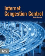
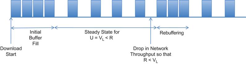
Video pictures, or frames, have to be played at a rate of about 30 frames per second (fps) to create the illusion of motion. Video compression is done by using the Discrete Cosine Transform (DCT) on the quantized grey scale and color components of a picture frame, and then transmitting the truncated DCT coefficients instead of the original picture. In addition to the intraframe compression, all compression algorithms also carry out interframe compression, which takes advantage of temporal picture redundancy in coding a frame by taking its delta with respect to a previous frame. Figure 6.1A shows a sequence of video frames, encoded using the Moving Picture Experts Group (MPEG) standard. There are three types of frames shown: I frames are largest because they only use intraframe compression; B and P frames are smaller because they use previous I frames to further reduce their size. This results in a situation in which the encoded bits per frame is a variable quantity, thus leading to Variable Bit Rate (VBR) video. Figure 6.1B shows the bits per frame for a sample sequence of frames.
A number of video coding standards are in use today: The most widely used is an ITU Standard called H.264 or MPEG-4; others include proprietary algorithms such as Google’s VP-9. Video coding technology has rapidly advanced in recent years, and today it is possible to send an HD-TV 1080p video using a bit rate of just 2 mbps.
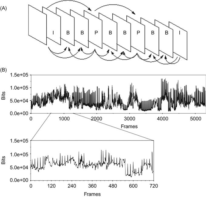
The encoded video results in a VBR stream that is then transmitted into the network (Figure 6.2). Because we are not depending on the network to provide a guaranteed bandwidth for the video stream, there arises the problem of matching the video bit rate with the bandwidth that the network can currently provide on a best-effort basis. If the network bandwidth is not sufficient to support the video bit rate, then the decoder at the receiving end starts to consume the video data at rate that is greater than the rate at which new data is being received from the network. As a result, the decoder ultimately runs out of video data to decode, which results in a screen freeze and the familiar “buffer loading” message that we often see. This is clearly not a good outcome, and to avoid this without having to introduce costly and complex guaranteed bandwidth mechanisms into the network, the following solutions try to match the video bit rate to the available network bandwidth:
• Use of a large receive buffer: As shown in Figure 6.2, the system can smooth out the variations in network throughput by keeping a large receive buffer. As a result, temporary reductions in throughput can be overcome by used the video stored in the receive buffer.
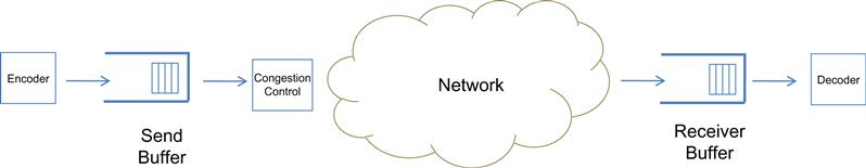
• Transcoding-based solutions (Figure 6.3A): These algorithms change one or more parameters of the compression algorithm that operates on the raw video data to vary the resulting bit rate. Examples include varying the video resolution, compression ratio, or frame rate. Transcoding is very CPU intensive and requires hardware support to be done at scale, which makes them difficult to deploy in Content Delivery Networks (CDN).
• Scalable encoding solutions (Figure 6.3B): These can be implemented by processing the encoded video data rather than the raw data. Hence, the raw video can be encoded once and then adapted on the fly by using the scalability features of the encoder. Examples of scalable encoding solutions include adapting the picture resolution or frame rate by exploiting the spatial or temporal scalability in the data. However, even scalable encoding is difficult to implement in CDNs because specialized servers are needed for this.
• Stream switching solutions (Figure 6.3C): This technique is the simplest to implement and can also be used by CDNs. It consists of preprocessing the raw video data to produce multiple encoded streams, each at a different bit rate, resulting in N versions. An algorithm is used at the time of transmission to choose the most appropriate rate given the network conditions. Stream switching algorithms use the least processing power because after the video is encoded, no further operations are needed. The disadvantages of this approach include the fact that more storage is needed and the coarser granularity of the encoded bit rates.
The industry has settled on using a large receive buffer and stream switching as the preferred solution for video transmission. Before the coding rate at the source can be changed, the video server has to be informed about the appropriate rate to use. Clearly, this is not a function that a congestion control protocol such as TCP provides; hence, all video transmissions systems define a protocol operating on top of TCP. In some of the early work on video transport, protocols such as Rate Adaptation Protocol (RAP) [2] and TFRC [1] were defined that put the sender in charge of varying the sending rate (and consequently the video rate) based on feedback being received from either the network or the receiver; hence, they were doing a combination of congestion control and flow control. For example, RAP used an additive increase/multiplicative decrease (AIMD)–type scheme that is reminiscent of TCP congestion control, and TFRC used an additive increase/additive decrease (AIAD) scheme that is based on the TCP square root formula.
The HAS protocol, which dominates video transport today, uses a scheme that differs from these early algorithms in the following ways:
• HAS is built on top of TCP transport, unlike the earlier schemes, which were based on UDP. Some of the reasons for using TCP were mentioned in the Introduction.
• Instead of the transmitter, the receiver in HAS drives the algorithm. It keeps track of the TCP rate of the video stream as well as the receive buffer occupancy level, and then using the HTTP protocol, it informs the transmitter about the appropriate video bit rate to use next.
• Instead of sending the video packets in a continuous stream, HAS breaks up the video into chunks of a few seconds each, each of which is requested by the receiver by means of an HTTP request.
HAS adapts the sending rate, and consequently the video quality, by taking longer term averages of the TCP transmit rate and variations in the receive buffer size. This results in a slower variation in the sending rate, as opposed to TCP congestion control, which varies the sending rate rapidly in reaction to network congestion or packet drops.
6.2.1 Constant Bit Rate (CBR) Video Transmission over TCP
To illustrate the transmission of video over packet networks, we will consider the simplest case of live CBR video transmission over a network with variable congestion (Figure 6.4). Let S(t)=Kt be the number of bits the source encoder has transmitted into the network by time t. If D(t) is the number of bits the receiving decoder has pulled from the receive buffer by time t, then
(1)
where ![]() is the delay before the decoder starts pulling data from the receive buffer. During this initial start-up time,
is the delay before the decoder starts pulling data from the receive buffer. During this initial start-up time, ![]() bits are transmitted by the encoder, which are in transit in the network or waiting to be decoded in the receive buffer.
bits are transmitted by the encoder, which are in transit in the network or waiting to be decoded in the receive buffer.
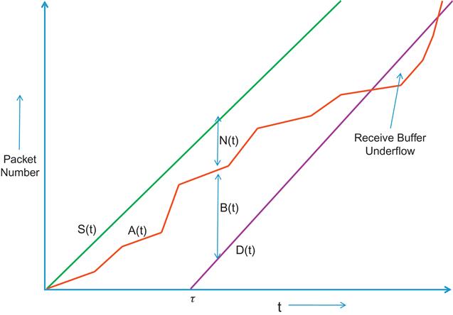
A(t): The number of bits that have arrived at the receive buffer
N(t): The number of bits in transit through the network
B(t): The number of bits waiting to be decoded in the receive buffer
Then
(2)
(3)
so that
(4)
which is a constant for ![]() .
.
Note that A(t) is dependent on the congestion state of the network, hence
• If the network is congestion free, then A(t) is close to S(t), so that the amount of traffic in the network ![]() by equation 2, and the amount of bits in the receiver is approximately given by
by equation 2, and the amount of bits in the receiver is approximately given by ![]() by equation 3, so that the receive buffer is full.
by equation 3, so that the receive buffer is full.
• If the network is congested, then A(t) begins to approach D(t), so that ![]() and
and ![]() by equations 3 and 4. In this situation, the decoder may run out of bits to decode, resulting in a frame freeze.
by equations 3 and 4. In this situation, the decoder may run out of bits to decode, resulting in a frame freeze.
If TCP is used to transport the CBR video stream, then to reduce the frequency of buffer underflows at the receiver, the designer can resort to policies such as:
1. Make sure that the network has sufficiently high capacity to support the video stream: Wang et al. [3] have shown that to support a CBR video stream of rate K bps, the throughput of the TCP stream transporting the video should be at least 2K bps. This ensures that the video does not get interrupted too frequently by frame freezes.
2. Use a sufficiently large receive buffer: Kim and Ammar [4] have shown that for a CBR stream of rate K, given a network characterized by a random packet drop rate p, round trip latency T, and retransmission timeout T0, the receive buffer size B that results in a desired buffer underrun probability Pu, is lower bounded by
(5)
 (5)
(5)
This result assumes that the CBR video rate K coincides with the average data rate that the TCP connection can support, so that

This last assumption is difficult to satisfy in practice, which may be reason why equation 5 is not commonly used to dimension receive buffers.
6.3 HTTP Adaptive Streaming (HAS)
The discussion in Section 6.2 showed that when TCP is used to transport CBR video, one can reduce the incidence of receive buffer exhaustion, either by overprovisioning the network so that the TCP rate is double the video rate or by using a sufficiently large receive buffer, which averages out the rate fluctuations attributable to TCP congestion control, but this begs the question of whether there are better ways of solving this problem that use less resources.
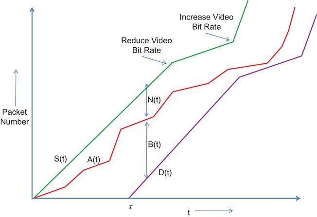
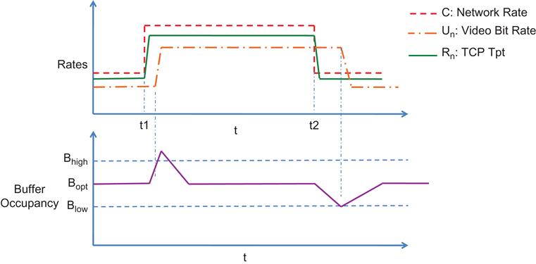
Most of the video streaming industry has now settled on HAS as the extra ingredient needed to send video over the Internet. HAS was able to improve the system by adding another layer of rate control on top of TCP. However, unlike TCP, the HAS algorithm is video aware and is able to interact with the video application at the sender to adaptively change its sending rate. The result of this interaction is shown in Figure 6.5, where one can see the video rate decreasing if the network congestion increases, and conversely increasing when the congestion reduces. As a result of this, the system is able to stream video without running into frame-freeze conditions and without having to overprovision the network or keep a very large receive buffer (compare Figure 6.5 with Figure 6.4 in which the receiving buffer underflows without bit rate adaptation). Note that Figure 6.5 assumes that the video is encoded at multiple rates, which can be adaptively changed depending on the network conditions.
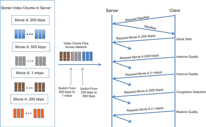
As mentioned in the Introduction, HAS uses HTTP/TCP for transporting video rather than the traditional RTP/UDP stack. With HAS, a video stream is divided into short segments of a few seconds each, referred to as chunks or fragments. Each chunk is encoded and stored in the server at a number of versions, each with a different bit rate as shown in Figure 6.6. At the start of the video session, a client downloads a manifest file that lists all the relevant information regarding the video streams. The client then proceeds to download the chunks sequentially using HTTP GETs. By observing the rate at which data is arriving to the client and the occupancy of the video decoding buffer, the client chooses the video bit rate of the next chunk. The precise algorithm for doing so is known as the ABR algorithm and is discussed in the next section.
Examples of commercial HAS systems that are in wide use today include the following:
• Microsoft HTTP Smooth Streaming (HSS) [5]: Uses a chunk size of 2 sec and a 30-sec receive buffer at the receiver
• Apple HTTP Live Streaming (HLS)
• Adobe HTTP Dynamic Streaming (HDS) [6]: Uses a receive buffer of size less than 10 sec
• Netflix [7]: Uses a chunk size of 10 sec and a 300-sec receive buffer
These HAS algorithms are proprietary to each vendor, which typically do not reveal details about their schemes. One can obtain some understanding of how they behave by carrying out measurements, and this program was carried out by Akhshabi et al. [8], from whom the numbers quoted here have been taken.
6.4 The Adaptive Bit Rate (ABR) Algorithm
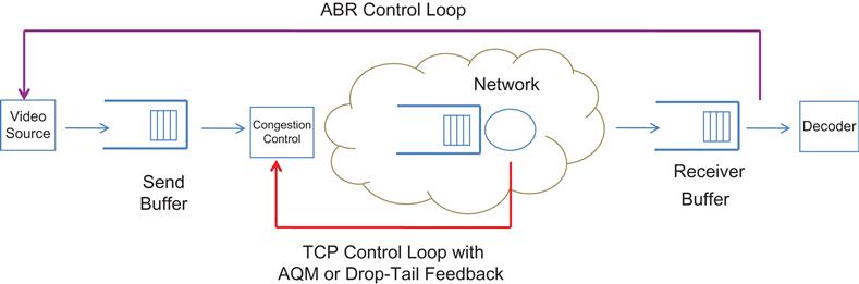
The ABR is the algorithm that HAS uses to adapt the video bit rate. With reference to Figure 6.7, while the TCP inner control loop reacts to network congestion and tries to match the TCP send rate with the rate that the network can support, the ABR outer loop reacts to the rates that TCP decides to use and tries to match the rate of the video stream to the average TCP rate. The TCP control loop operates in order of a time period, which is approximately equal to the round trip delay (i.e., tens of milliseconds in most cases); the ABR control loop operates over a much larger time period, ranging from a few seconds to tens of seconds depending on the ABR algorithm. This leads to a natural averaging effect because ABR does not attempt to match the fluctuating short-term TCP throughput but rather a smoothed throughput that is averaged over several seconds. Even then, it is a nontrivial problem to estimate the “true” average TCP rate from measurements made at the receiver [9], and we shall see later that ABR’s transmission policy can lead to an overestimation of TCP throughput, which results in oscillations in the video rate.
The ABR algorithm controls the following quantities:
• The rate at which the receiver sends HTTP requests back to the video source
• The appropriate video stream to transmit, whose rate most closely matches the rate that can be supported by the network
The objectives of an ideal ABR algorithm include the following:
1. Avoid interruptions of playback caused by buffer underruns.
2. Maximize the quality of the video being transmitted: Fulfilling this objective constitutes a trade-off with objective 1 because it is always possible to minimize the number of interruptions by always transmitting at the lowest rate.
3. Minimize the number of video quality shifts to improve user experience: This leads to a trade-off with objective 2 because the algorithm can maximize the video quality by reacting to the smallest changes in the network bandwidth, which, however, increases the number of quality shifts.
4. Minimize the time between the user making a request for a new video and the video actually starting to play: This objective can also be achieved at the cost of objective 2 by using the lowest bit rate at the start.
![]() Set of available bit rates for the video stream that are available at the transmitter, with 0<V(n)<V(m) for n<m
Set of available bit rates for the video stream that are available at the transmitter, with 0<V(n)<V(m) for n<m
![]() : The video rate from the set V which is used for the nth chunk, which is an output of the ABR algorithm
: The video rate from the set V which is used for the nth chunk, which is an output of the ABR algorithm
![]() : Size of a chunk in seconds, in terms of actual time spent in playing the video contained in it
: Size of a chunk in seconds, in terms of actual time spent in playing the video contained in it
![]() : Throughput for the nth video chunk as measured at the receiver
: Throughput for the nth video chunk as measured at the receiver
![]() : HTPP inter-request interval, between the nth and (n+1)rst requests. This is also an output of the ABR algorithm.
: HTPP inter-request interval, between the nth and (n+1)rst requests. This is also an output of the ABR algorithm.
![]() : Download duration for the nth chunk
: Download duration for the nth chunk
![]() : Actual inter-request time between HTTP requests from the receiver, between the nth and (n+1)rst request, so that
: Actual inter-request time between HTTP requests from the receiver, between the nth and (n+1)rst request, so that
(6)
This is also referred to as the nth download period.
Because the size of the receive buffer is in terms of the duration of video data stored in it, the download of a chunk causes the buffer size to increase by ![]() seconds irrespective of the rates Un or Rn. Similarly, it always takes
seconds irrespective of the rates Un or Rn. Similarly, it always takes ![]() seconds to play the video data in a chunk, irrespective of the rate at which the video has been coded.
seconds to play the video data in a chunk, irrespective of the rate at which the video has been coded.
Most ABR algorithms use the following three steps:
1. Estimation: The throughput during the nth video chunk is estimated using the following equation:
(7)
The buffer size (in seconds) at the end of the nth download period is computed by
(8)
2. Video rate determination: The ABR algorithm determines the rate Un+1 to be used for the next chunk by looking at several pieces of information, including (1) the sequence of rate estimates Rn and (2) the buffer occupancy level Bn. Hence,
(9)
where F(.) is a rate determination function.
3. Scheduling: The ABR algorithm determines the time when the next chunk is scheduled to be downloaded at by computing an HTTP inter-request time of ![]() , such that
, such that
(10)
Note that equation 7 assumes that the video rate is fixed at Un for the duration of the nth chunk. In reality, it may vary, and we can take this into account by replacing ![]() by
by ![]() , which is the number of bits received as part of the nth chunk.
, which is the number of bits received as part of the nth chunk.
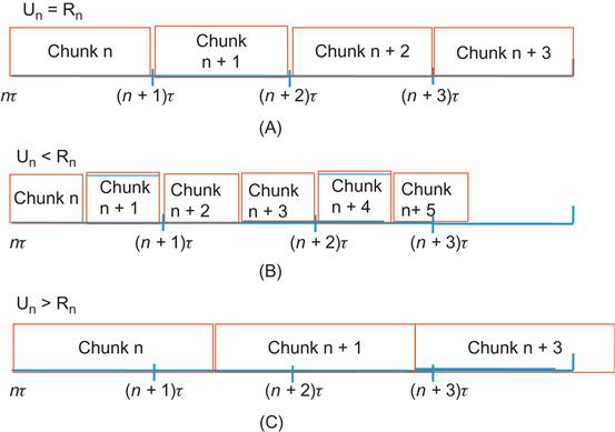
Figure 6.8A shows the downloading of multiple video chunks at the receiver. As noted earlier, the time spent in playing the video contained in a chunk is always ![]() seconds; however, the time required to transmit a chunk is variable and is given by equation 7. Keeping in mind that
seconds; however, the time required to transmit a chunk is variable and is given by equation 7. Keeping in mind that
it follows that (see Figure 6.8), if
• Rn=Un (Figure 6.8A): Because the two rates are perfectly matched, it takes exactly ![]() seconds to transmit the chunk, and there is no change in the buffer size at end of the nth period (by equation 8). This is ideal state for the ABR algorithm because it makes full use of the network capacity, and the buffer size is steady. Note that in practice, this perfect match does not occur because of the quantization in the video bit rates.
seconds to transmit the chunk, and there is no change in the buffer size at end of the nth period (by equation 8). This is ideal state for the ABR algorithm because it makes full use of the network capacity, and the buffer size is steady. Note that in practice, this perfect match does not occur because of the quantization in the video bit rates.
• Rn>Un (Figure 6.8B): In this case, ![]() , so the network fills up the buffer faster (two chunks every
, so the network fills up the buffer faster (two chunks every ![]() seconds) than the constant rate at which the decoder is draining it (one chunk every
seconds) than the constant rate at which the decoder is draining it (one chunk every ![]() seconds). This condition needs to be detected by the ABR algorithm so that it can take control action, which consists of increasing the video bit rate so that it can take advantage of the higher network capacity. If the video bit rate is already at a maximum, the ABR algorithm avoids buffer overflow by spacing out the time interval between chunks (see Figure 6.10).
seconds). This condition needs to be detected by the ABR algorithm so that it can take control action, which consists of increasing the video bit rate so that it can take advantage of the higher network capacity. If the video bit rate is already at a maximum, the ABR algorithm avoids buffer overflow by spacing out the time interval between chunks (see Figure 6.10).
• Rn<Un (Figure 6.8C): In this case, ![]() so the decoder drains the buffer at a higher rate than the rate at which the network is filling it, which can result in an underflow. This condition also needs to be detected promptly by the ABR algorithm so that it can take control action, which consists of reducing the video bit rate to a value that is lower than the network rate.
so the decoder drains the buffer at a higher rate than the rate at which the network is filling it, which can result in an underflow. This condition also needs to be detected promptly by the ABR algorithm so that it can take control action, which consists of reducing the video bit rate to a value that is lower than the network rate.
To understand the dynamics of ABR algorithms, consider the scenario pictured in Figure 6.9. Assume that the TCP throughput is fixed and is given by R, and furthermore, it lies between the video rates V(m) and V(m+1).
• If the ABR algorithm chooses rates Un that are V(m+1) or larger, then this will result in the scenario shown in Figure 6.9B, in which the decoder drains the buffer faster than the rate at which the network is filling it, resulting in a decreasing buffer size. If left unchecked, then this will eventually result in an underflow of the receive buffer.
• If the ABR algorithm chooses rates Un that are equal to V(m) or smaller, then this will result in the scenario shown in Figure 6.9C, in which the network fills the buffer faster than the rate at which the decoder can drain it. This will result in an increasing buffer size.
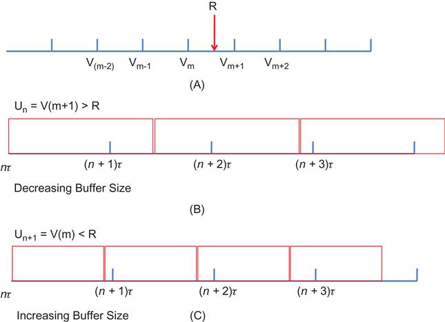
Because of the quantization in video rates, it is impossible to get to Un=R, and this can result in the video rate constantly fluctuating between V(m) and V(m+1) to keep the buffer from overflowing or underflowing. To avoid this, most ABR algorithms stop increasing the video rate Un after it gets to V(m) and compensate for the difference between V(m) and R by increasing the gap between successive downloads, as shown next.
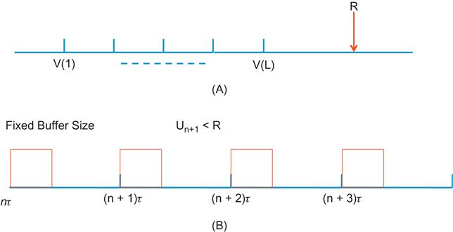
The case when the TCP throughput R exceeds the maximum video rate V(L) (Figure 6.10A) will result in the system dynamics shown in Figure 6.9C in which the receive buffer size keeps increasing. If the ABR algorithm observes that the buffer size is increasing even at the maximum video bit rate, then it stabilizes the buffer by increasing the gap between successive downloads, as shown in Figure 6.10B. There are two ways in which it can choose the gap size:
• The gap size is fixed at ![]() : In this case, during each period, the amount of video data consumed is equal to the data being added, resulting in a stable buffer.
: In this case, during each period, the amount of video data consumed is equal to the data being added, resulting in a stable buffer.
• After the end of the chunk download, the ABR algorithm waits for the buffer to drain until it reaches a target level before starting the next download.
At a high level, the ABR algorithm tries to match the rate at which the receive buffer is being drained by the video decoder (i.e., the sequence {Un}), with the rate at which this buffer is being replenished by the network (i.e., the sequence {Rn}) in a way such that the receive buffer does not become empty. This is difficult problem because the rate at which the buffer is being filled is constantly fluctuating because it is determined by TCP’s congestion control algorithm as a function of the congestive state of the network. This problem is made harder because buffer fluctuations may also be caused by the VBR nature of the video stream.
It does not makes sense to constantly keep changing the video bit rate in response to network rate changes because studies have shown that switching back and forth between different video versions significantly degrades the user experience. Hence, one of the objectives of the ABR algorithms is to avoid video rate fluctuations caused by short-term bandwidth variations and TCP throughput estimation errors. In general, it has been observed that whereas algorithms that try to keep the buffer size stable cause larger variations in the video bit rate, algorithms that try to keep the video bit rate stable lead to larger variations in the buffer size. Several techniques are used to smoothen out the video rate fluctuations, such as:
• Use the receive buffer to dampen out temporary fluctuations in TCP bit rate: This is illustrated by the Threshold Based Buffer (TBB) algorithm [10] (see Section 6.5.2.1).
• Use smoothing filters to reduce fluctuations in the TCP bit rate estimates. This is illustrated by the STB algorithm (see Section 6.5.1.3).
Even though it is not a congestion control algorithm, most ABR designs conform to the AIMD rules. Hence, the video bit rate is incremented smoothly in an additive manner when the available network bandwidth is consistently higher than the current bit rate. Conversely, when the network bandwidth decreases because of congestion, ABR should quickly decrease the video bit rate to avoid playback freezes. Another reason to use multiplicative decrease for the video rate is the following: In case of congestion, the TCP reacts by multiplicatively reducing its own bit rate, and because the objective of the ABR algorithm is to match the video bit rate to the TCP throughput, it follows that it should also try to reduce the video bit rate multiplicatively.
6.5 Description of Some Adaptive Bit Rate (ABR) Algorithms
Adaptive Bit Rate or ABR algorithms are an active area of research, and new algorithms are being constantly invented in both academia and industry. These can be broadly classified in the following categories:
1. Algorithms that rely mostly on their estimates of TCP throughput. Algorithms in this category include:
• Network Throughput Based (NTB)
• Smoothed Throughput Based (STB) [8]
• AIMD Based (ATB) [11]
• The FESTIVE algorithm [12]
2. Algorithms that rely mostly on the receive buffer size. Algorithms in this category include:
• Threshold Based Buffer (TBB) [10]
• Buffer Based Rate Selection (BBRS) [13]
3. Control Theory Based (CTB) [14–16]
These algorithms estimate the best video bit rate to use by solving a control theory problem.
In the research literature, there are algorithms that rely on the Send buffer size to control the video bit rate [17]. These algorithms have some inherent disadvantages compared with the receiver-based algorithms, including that they increase the complexity and cost of the video server. Also, the benefits of caching the content in a distributed fashion are lost. Hence, these types of algorithms are not covered in this chapter.
6.5.1 Throughput-Based Adaptive Bit Rate (ABR) Algorithms
This class of algorithms uses estimates of the TCP throughput as the main input to the algorithm. However, all such algorithms also incorporate a safety feature whereby if the receive buffer size falls below a threshold, then the system switches the video bit rate to the minimum value to avoid a buffer underflow.
6.5.1.1 Network Throughput-Based (NTB) Algorithm
This is the simplest type of ABR algorithm. Essentially, the video bit rate for the next download is set equal to the latest value of the TCP throughput estimate, so that
(11)
The quantization function Q chooses the video bit rate that is smaller than Rn and closest to it. Note that equation 11 cancels out the instantaneous fluctuations in TCP throughput by averaging over an interval, which is typically 2 to 10 seconds long. The NTB algorithm is very effective in avoiding buffer underruns because it reacts instantaneously to fluctuations in TCP throughput. Studies have shown that receive buffer size shows the least amount of variation under NTB compared with the other algorithms [18]. However, on the flip side, it has the largest rate of changes in the video bit rate because it does nothing to dampen any of these fluctuations. As a result, it is not commonly used in practice except as a way to benchmark other ABR algorithms.
Figure 6.11 shows an example a typical sample path of the NTB algorithm. The video rate is typically set to the minimum value V(1) at start-up, but it quickly increases to the maximum bit rate V(L) because of application of equation 11. Downloads are done in a back-to-back manner until the receive buffer is full. When this happens, the download interval is increased to ![]() seconds to keep the average TCP throughput R equal to V(L). If the TCP throughput falls below V(L), then the receive buffer occupancy starts to reduce, and the algorithm switches to the back-to-back downloads again. This takes the system to the scenario illustrated in Figure 6.9, where in the absence of any smoothing, the algorithm will constantly switch between the bit rates that are above and below R.
seconds to keep the average TCP throughput R equal to V(L). If the TCP throughput falls below V(L), then the receive buffer occupancy starts to reduce, and the algorithm switches to the back-to-back downloads again. This takes the system to the scenario illustrated in Figure 6.9, where in the absence of any smoothing, the algorithm will constantly switch between the bit rates that are above and below R.
6.5.1.2 AIMD-Based Algorithm (ATB)
The ATB algorithm [11] makes a number of modifications to the NTB algorithm to smoothen out the bit rate fluctuations. Using the same notation as before, the ATB algorithm keeps track of the ratio ![]() given by
given by
(12)
Note that because ![]() , if
, if ![]() , then the video bit rate is larger than the TCP throughput, and the converse is true when
, then the video bit rate is larger than the TCP throughput, and the converse is true when ![]() . Hence,
. Hence, ![]() serves as a measure of network congestion.
serves as a measure of network congestion.
The bit rate increment–decrement rules are as follows:
• If ![]() (and the buffer size exceeds a threshold) where
(and the buffer size exceeds a threshold) where ![]() , then the chunk download happens faster than the rate at which the decoder can play that chunk (see Figure 8B). The video bit rate is switched up from V(m) to V(m+1), which corresponds to an additive increase policy. Hence, in contrast to NTB, the ATB algorithm increases the bit rate using an additive increase policy, which helps to reduce jumps in video quality. Also, the factor
, then the chunk download happens faster than the rate at which the decoder can play that chunk (see Figure 8B). The video bit rate is switched up from V(m) to V(m+1), which corresponds to an additive increase policy. Hence, in contrast to NTB, the ATB algorithm increases the bit rate using an additive increase policy, which helps to reduce jumps in video quality. Also, the factor ![]() helps to reduce bit rate oscillations for the case when the TCP throughput lies between two video bit rates (illustrated in Figure 6.9A).
helps to reduce bit rate oscillations for the case when the TCP throughput lies between two video bit rates (illustrated in Figure 6.9A).
• If ![]() , where
, where ![]() is the switch-down threshold, then the download of a chunk takes longer than the time required for the decoder to play that chunk, which leads to a reduction in the receive buffer size. Hence, an aggressive switch down is performed, with the reduced video bit rate chosen to be the first rate V(i) such that
is the switch-down threshold, then the download of a chunk takes longer than the time required for the decoder to play that chunk, which leads to a reduction in the receive buffer size. Hence, an aggressive switch down is performed, with the reduced video bit rate chosen to be the first rate V(i) such that ![]() , where V(c) is the current bit rate. This corresponds to a multiplicative decrease policy. The presence of the factor
, where V(c) is the current bit rate. This corresponds to a multiplicative decrease policy. The presence of the factor ![]() may lead to the situation in which the buffer drains down slowly. To prevent an underflow, the algorithm switches to the minimum bit rate V(1) if the buffer falls below a threshold.
may lead to the situation in which the buffer drains down slowly. To prevent an underflow, the algorithm switches to the minimum bit rate V(1) if the buffer falls below a threshold.
From this description, the ATB algorithm uses fudge factors in its threshold rules and a less aggressive increase rate to reduce bit rate fluctuations. If the TCP throughput exceeds the maximum video bit rate, then it spaces out the chunk download times to prevent the buffer from overflowing.
6.5.1.3 Smoothed Throughput Based (STB) Algorithm
To reduce the short-term fluctuations in the NTB algorithm, the STB algorithm [8] uses a smoothed throughput estimate, as follows:
(13)
where Rn is given by (11), followed by
As a result of the smoothing, the STB algorithm considerably reduces the number of changes to the video bit rate in response to TCP throughput fluctuations. However, if there is a sudden decrease in TCP throughput, STB is not able to respond quickly enough, which can result in buffer underflows. However, if the buffer size is big enough, then STB provides a simple and viable ABR technique. The interval between chunks is controlled in the same way as in the NTB algorithm.
6.5.1.4 The FESTIVE Algorithm
Jiang et al. [12] pointed out the following problems that exist in ABR algorithms that are caused due to their measurements of TCP throughput to control the video bit rates:
• The chunk download start-time instances of the connections may get stuck in suboptimal locations. For example, if there are three active connections, then the chunk download times of two of the connections may overlap, while the third connection gets the entire link capacity. This leads to unfairness in the bit rate allocation.
Their suggested solution is to randomize the start of the chunk download times; that is, instead of downloading a chunk strictly at intervals of ![]() seconds (or equivalently when the buffer size reaches a target value), move it randomly either backward or forward by a time equal to the length of download.
seconds (or equivalently when the buffer size reaches a target value), move it randomly either backward or forward by a time equal to the length of download.
• Connections with higher bit rate tend to see a higher estimate of their chunk’s TCP throughput. As explained in Section 6.5.2, this is because the chunks of connections with higher bit rates occupy the bottleneck link longer, and as a result, they have a greater chance of experiencing time intervals during which they have access to the entire link capacity.
To solve this problem, Jiang et al. [12] recommended that the rate of increase of the bit rate for a connection should not be linear but should decrease as the bit rate increases (another instance of the averaging principle!). This policy can be implemented as follows: If the bit rate is at level k, then increase it to level k+1 only after k chunks have been received. This will lead to a faster convergence between bit rates of two connections that are initially separated from each other.
• Simple averaging of the TCP throughput estimates is biased by outliers if one chunk sees a very high or very low throughput. To avoid this, Jiang et al. [12] implemented a harmonic mean estimate of the last 20 throughput samples, which is less sensitive to outliers.
As a result of these design changes, the HAS design using the FESTIVE algorithm was shown to outperform the commercial HAS players by a wide margin.
6.5.2 Buffer Size-Based Adaptive Bit Rate Algorithms
This class of algorithms uses receive buffer size as their primary input, although most of them also use the TCP throughput estimate to do fine tuning. It has been recently shown (see Section 6.5.3) that buffer size–based ABR algorithms outperform those based on rate estimates.
6.5.2.1 Threshold Based Buffer (TBB) Algorithm
The following rules are used for adapting the video bit rate in the TBB algorithm [10]:
• Let B(t) be the receive buffer level at time t. Define the following threshold levels for the receive buffer, measured in seconds: ![]() . The interval
. The interval ![]() is called the target interval, and
is called the target interval, and ![]() is the center of the target interval. The TBB algorithm tries to keep the buffer level close to Bopt.
is the center of the target interval. The TBB algorithm tries to keep the buffer level close to Bopt.
• Let V(c) be the current video bit rate. If the buffer level B(t) falls below Blow and ![]() , then switch to the next lower bit rate V(c−1). The algorithm continues to switch to lower bit rates as long as the above conditions are true. Note that if B(t)<Blow and
, then switch to the next lower bit rate V(c−1). The algorithm continues to switch to lower bit rates as long as the above conditions are true. Note that if B(t)<Blow and ![]() , it implies that the buffer level has started to increase, and hence there is no need to switch to a lower rate.
, it implies that the buffer level has started to increase, and hence there is no need to switch to a lower rate.
• With the current video bit rate equal to V(c), if the buffer level increases above Bhigh and if ![]() , then switch to the next higher video bit rate V(c+1). Note that
, then switch to the next higher video bit rate V(c+1). Note that ![]() is the average TCP throughput, where the average is taken over the last few chunks (this number is configurable), which helps to dampen temporary network fluctuations.
is the average TCP throughput, where the average is taken over the last few chunks (this number is configurable), which helps to dampen temporary network fluctuations.
If the video bit rate is already at the maximum value V(L) or if
(14)
then the algorithm does not start the download of the next chunk until the buffer level B(t) falls below ![]() . Assuming that initially
. Assuming that initially ![]() , this policy leads to a steady linear decrease in buffer size by
, this policy leads to a steady linear decrease in buffer size by ![]() every
every ![]() seconds until it reaches the target operating point Bopt. If equation 14 is satisfied, then it means that the bit rates V(c) and V(c+1) straddle the TCP throughput (as in Figure 6.9A) so that increasing the bit rate to V(c+1) will cause the buffer to start decreasing.
seconds until it reaches the target operating point Bopt. If equation 14 is satisfied, then it means that the bit rates V(c) and V(c+1) straddle the TCP throughput (as in Figure 6.9A) so that increasing the bit rate to V(c+1) will cause the buffer to start decreasing.
• If ![]() , the algorithm does not change the video bit rate to avoid reacting to short-term variations in the TCP throughput. If the bit rate is at maximum value V(L) or if equation 14 is satisfied, then the algorithm does not start the download of the next chunk until the buffer level B(t) falls below
, the algorithm does not change the video bit rate to avoid reacting to short-term variations in the TCP throughput. If the bit rate is at maximum value V(L) or if equation 14 is satisfied, then the algorithm does not start the download of the next chunk until the buffer level B(t) falls below ![]() . This keeps the buffer level at Bopt in equilibrium.
. This keeps the buffer level at Bopt in equilibrium.
• If the buffer level falls below Bmin, then switch to the lowest video bit rate to V(1).
Simulation results presented by Miller et al. [10] show that the algorithm works quite well and achieves its objectives. Figure 6.12 shows a sample path of the algorithm for the case when Bhigh=50 sec, Blow=20 sec (so that Bopt=30 sec), and Bmin=10 sec, with a single video stream passing over a network bottleneck link whose capacity is varied.
• When the link capacity goes up at t1 = 200 sec, the buffer size starts to increase, and when it crosses 50 sec, the algorithm starts to increase the bit rate in multiple steps. When the bit rate reaches the maximum value, the algorithm reduces the buffer size linearly until it reaches Bopt.
• When the link capacity is reduced at t2 = 400 sec, it causes the buffer occupancy to decrease, and when it drops below 20 sec, the video bit rate is progressively decreased until it falls below the TCP throughput value. At this point, the buffer starts to fill up again, and when it reaches Bopt, the algorithm spaces out the chunks to maintain the buffer at a constant value.
A nice feature of the TBB algorithm is that it enables the designer to explicitly control the trade-off between variation in buffer occupancy and fluctuations in video bit rate in response to varying TCP throughput. This is done by controlling the thresholds Bhigh and Blow, such that a large value of the difference Bhigh–Blow will reduce video bit rate changes. This aspect of TBB is orthogonal to the features in the FESTIVE algorithm, and a combination of the two will result in a superior system.
6.5.2.2 Buffer Based Rate Selection Algorithm
The BBRS algorithm [13] bases its bit rate selection function entirely on the receive buffer level. This function is illustrated in Figure 6.13. It sets the video bit rate to Q(Un), where Un is defined by:
(15a)
(15b)
(15c)
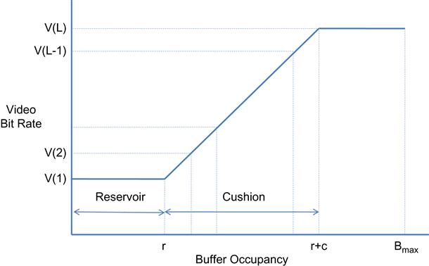
Note that r and c are free parameters in this algorithm. The algorithm makes the implicit assumption that the maximum TCP throughput is bounded between V(1) and V(L), so that all chunk downloads always happen in a back-to-back manner. This also implies that if the TCP rate R lies between video bit rate Vm and Vm+1 (see Figure 6.9), then the buffer occupancy with constantly switch back and forth between f−1(Vm) and f−1(Vm+1) (where f is the mapping function shown in Figure 6.13), which will result in the video bit rate switching between these two values as well. The TBB algorithm avoids this by keeping track of the TCP throughput in addition to the buffer occupancy, as explained in the previous section.
6.5.3 Control Theory–Based Adaptive Bit Rate Algorithms
Inspired by the success of control theory in analyzing congestion control (see Chapter 3), several researchers have attempted to use this theory to derive ABR algorithms [14–16]. The initial work by Tian and Liu [15] and Zhou et al. [16] was based the objective of controlling the receive buffer occupancy to a reference level Bref and then using the difference (Bn–Bref) between the current occupancy and the reference value to drive the main control loop as shown in Figure 6.14. (Note the analogy with the TCP case in which the objective of the controller was to regulate the bottleneck buffer occupancy to some reference level.) It is then possible to derive equations for the predicted video bit rate Un as a function of the buffer size difference and the estimated TCP throughput Rn, which in turn determines the buffer occupancy level in combination with the actual TCP throughput, thus closing the control loop.
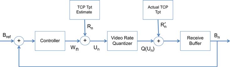
In general, it turns out that trying to keep the receive buffer occupancy at the reference level is not the most suitable way to drive the ABR control loop. The reason for this is the fact that from a user point of view, it is more important to get the highest quality video that the network can support while reducing the bit rate fluctuations. The user does not care if the buffer is fluctuating as long as it does not underflow. The model in Figure 6.14 does not take into account the objectives of reducing the bit rate fluctuations or maximizing the video quality. In their algorithms, Tian and Liu [15] and Zhou et al. [16] did include features to reduce the rate fluctuations, but this was done as an add-on to the control loop, not as a consequence of the control model itself.
Recently, Yin et al. [14] have attacked the problem using tools from model predictive control (MPC) theory with much better results, and their work is described in this section. In addition to taking multiple constraints into account in the derivation of the optimal bit rate, the theory also provides a framework within which different algorithms can be compared with the performance of the best possible ABR algorithm, thus enabling us to objectively compare different algorithms.
The MPC optimization problem is defined next. We will use the same notation that was introduced in Section 6.4, with the following additions:
K: Total number of chunks in the video stream so that the duration of the video is ![]() seconds
seconds
q(.): R→R+ This is a function that maps the selected bit rate Uk to the video quality perceived by the user q(Uk). It is assumed to be monotonically increasing.
The download of chunk k starts at time tk and finishes at time tk+1, and the download of the next chunk starts at time tk+1 (i.e., it is assumed that chunks are downloaded in a back-to-back manner); this implies that the maximum TCP throughput is less than the maximum video bit rate V(L). It follows that
(16)
(17)
 (17)
(17)
(18)
 (18)
(18)
where Bk=B(tk). Note that if ![]() , then the buffer becomes empty before the next download is complete, thus resulting in an underflow.
, then the buffer becomes empty before the next download is complete, thus resulting in an underflow.
Define the following Quality of Experience (QoE) elements for the system:
Or number of rebufferings: ![]()
The QoE of video segments 1 through K are defined by a weighted sum of these components
(19)
By changing the values of ![]() and
and ![]() , the user can control the relative importance assigned to video quality variability versus the frequency or time spent on rebuffering. Note that this definition of QoE takes user preferences into account and can be extended to incorporate other factors.
, the user can control the relative importance assigned to video quality variability versus the frequency or time spent on rebuffering. Note that this definition of QoE takes user preferences into account and can be extended to incorporate other factors.
The bit rate adaptation problem, called ![]() , is formulated as follows:
, is formulated as follows:
(20)
such that
The input to the problem is the bandwidth trace ![]() , which is a random sample path realization from the stochastic process that controls TCP throughput variations during the download.
, which is a random sample path realization from the stochastic process that controls TCP throughput variations during the download.
The outputs of ![]() are the bit rate decisions U1,…,UK, the download times t1,…,tK and the buffer occupancies B1,…,BK.
are the bit rate decisions U1,…,UK, the download times t1,…,tK and the buffer occupancies B1,…,BK.
Note that ![]() is a finite-horizon stochastic optimal control problem, with the source of the randomness being the TCP throughput R(t). At time tk when the ABR algorithm is invoked to choose Uk, only the past throughputs
is a finite-horizon stochastic optimal control problem, with the source of the randomness being the TCP throughput R(t). At time tk when the ABR algorithm is invoked to choose Uk, only the past throughputs ![]() are known; the future throughputs
are known; the future throughputs ![]() are not known. However, algorithms known bandwidth predictors can be used to obtain predictions defined as
are not known. However, algorithms known bandwidth predictors can be used to obtain predictions defined as ![]() . Several bandwidth predictors using filtering techniques such as AR (autoregressive), ARMA (autoregressive moving average), autoregressive integrated moving average (ARIMA), fractional ARIMA (FARIMA), and so on are known, which are all combinations of moving average and autoregressive filtering [19]. Based on this, the ABR algorithm selects bit rate of the next chunk k as:
. Several bandwidth predictors using filtering techniques such as AR (autoregressive), ARMA (autoregressive moving average), autoregressive integrated moving average (ARIMA), fractional ARIMA (FARIMA), and so on are known, which are all combinations of moving average and autoregressive filtering [19]. Based on this, the ABR algorithm selects bit rate of the next chunk k as:
(21)
Model predictive control [20] is a subset of this class of algorithms that choose bit rate Uk by looking h steps ahead; that is, they solve the QoE maximization problem ![]() with bandwidth predictions
with bandwidth predictions ![]() to obtain the bit rate Uk. The bit rate Uk is then applied to the system, and that along with the actual observed TCP throughput Rk is used to iterate the optimization process to the next step k+1.
to obtain the bit rate Uk. The bit rate Uk is then applied to the system, and that along with the actual observed TCP throughput Rk is used to iterate the optimization process to the next step k+1.
For a given TCP throughput trace ![]() , we can obtain the offline optimal QoE, denoted as QoE(OPT) (which is obtained by solving
, we can obtain the offline optimal QoE, denoted as QoE(OPT) (which is obtained by solving ![]() ) because it has perfect knowledge of the future TCP throughputs for the entire duration of the video streaming. This provides a theoretical upper bound for all algorithms for a given throughput trace.
) because it has perfect knowledge of the future TCP throughputs for the entire duration of the video streaming. This provides a theoretical upper bound for all algorithms for a given throughput trace.
Define QoE(A) to be the QoE for algorithm A and the normalized QoE of A as
(22)
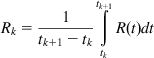
Yin et al. [14] generated several synthetic TCP throughput traces and used it to compute n-QoE(A) for the MPC algorithm, as well as the BBRS algorithm (as a representative of buffer-based algorithms) and the NTB algorithm (as a representative of throughput-based algorithms). Their results are very interesting and are summarized in Figure 6.15, which graphs the distribution function for n-QoEs from 100 simulation runs. It shows that BBRS performs better than NTB, and both are outperformed by the MPC algorithm, which gets quite close to the optimal.
6.6 The Problem with TCP Throughput Measurements
TCP throughput measurements form an essential component of the ABR algorithm. Algorithms such as ATB and STB use these measurements as their main input, and even algorithms such as TBB or BBRS that are based on buffer size measurements are affected by TCP throughput because the transmit time of a chunk (which determines whether the buffer grows or shrinks) is inversely proportional to the TCP throughput.
Recall that the ABR algorithms estimates the per-chunk TCP throughput using the formula
Consider the case when ABR-controlled video streams pass through a common network bottleneck node with capacity C and assume that the maximum video bit rate ![]() and
and ![]() . When only one of the video streams is active, it will result in the scenario shown in Figure 6.10 where there is a gap between successive chunks in steady state. When both the video streams become active, then their chunks can get distributed according to one of the scenarios shown in Figure 6.16. In case (A) in the figure, there is no overlap between the chunks at the bottleneck, which implies that each stream gets the full bottleneck bandwidth (i.e.,
. When only one of the video streams is active, it will result in the scenario shown in Figure 6.10 where there is a gap between successive chunks in steady state. When both the video streams become active, then their chunks can get distributed according to one of the scenarios shown in Figure 6.16. In case (A) in the figure, there is no overlap between the chunks at the bottleneck, which implies that each stream gets the full bottleneck bandwidth (i.e., ![]() ). In case (B), there is partial overlap, so that
). In case (B), there is partial overlap, so that ![]() , i=1,2. In case (C), there is full overlap so that
, i=1,2. In case (C), there is full overlap so that ![]() .
.
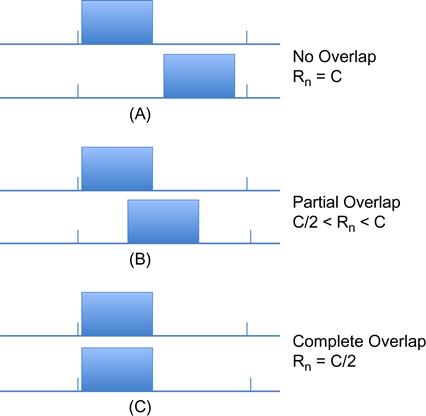
Hence, only in case c does the TCP throughput measurement reflect the ideal allocation of bottleneck bandwidth between the two sources. This effect, which was first pointed out by Akhshabi et al. [9], is attributable to the fact that ABR bunches together video packets into chunks for transmission. If the video sources are allowed to transmit continuously, then this effect goes away.
Li et al. [21] carried out a simulation study with 100 sources sharing a bottleneck node of capacity 100 mbps. For the case of an ABR interdownload time of ![]() seconds, the transmissions were randomly distributed between 0 and 2 seconds. The TCP throughput was measured using equation 7 using various values of link subscription and is shown in Figure 6.17. It shows the same behavior that we observed for two sources: If the link utilization is less than 100%, then the measured throughput is much higher than the fair bandwidth allocation (about three times the fair-share bandwidth in this example). This causes ABR to increase the video bit rate allocations. As a result of this, the link subscription soon rises above 100%, which causes the TCP throughput to fall precipitously, and the cycle repeats. This behavior has been christened the “bandwidth cliff” effect by Li et al. [21]
seconds, the transmissions were randomly distributed between 0 and 2 seconds. The TCP throughput was measured using equation 7 using various values of link subscription and is shown in Figure 6.17. It shows the same behavior that we observed for two sources: If the link utilization is less than 100%, then the measured throughput is much higher than the fair bandwidth allocation (about three times the fair-share bandwidth in this example). This causes ABR to increase the video bit rate allocations. As a result of this, the link subscription soon rises above 100%, which causes the TCP throughput to fall precipitously, and the cycle repeats. This behavior has been christened the “bandwidth cliff” effect by Li et al. [21]
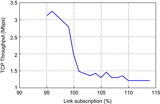
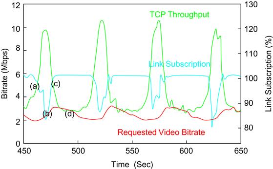
Figure 6.18 illustrates the periodic variation in the TCP throughput estimates, the video bit rates and the utilization of the bottleneck link capacity, caused by the bandwidth cliff. Li et al. [21] have recently designed an ABR algorithm called PANDA to avoid the bandwidth cliff effect. The FESTIVE algorithm uses randomization of the chunk download start times to avoid this problem.
By considerations similar to that used for Figure 6.16, it follows that if two HAS sessions are sharing a link and one of them has higher bit rate than the other, then the TCP throughput estimate for the higher bit rate connection will also be higher than that of the lower bit rate connection, which results in unfairness. This is because the higher bit rate connection occupies the link for a longer time, and as a result there are periods when it has access to the entire link bandwidth, thus pushing up its TCP throughput. This problem was first pointed out by Jiang et al. [12], who also proposed a solution for it in their FESTIVE algorithm.
6.7 Interaction Between TCP and ABR
In recent years, streaming video has become the dominant form of traffic on the Internet, and as result, video rate control algorithms such as ABR are probably more important than traditional TCP congestion control in understanding the dynamics and evolution of Internet traffic. One of the important issues that researchers have started to investigate only recently is How does ABR rate control interact with TCP congestion control, and how do multiple ABR-controlled streams interact with one another? These topics are discussed in the following two subsections, but in this section, we will describe the consequences of using TCP for transporting individual HAS chunks.
The video stream is sent in a series of individual chunks over TCP, which results in the following issues:
1. The TCP window size that is reached at the end of chunk n serves as the initial window size for chunk (n+1). As a result, when the chunk (n+1) transmission starts, up to W TCP segments are transmitted back to back into the network (where W is the TCP window size). For large values of n, this can overwhelm buffers at congested nodes along the path and result in buffer overflows.
2. Assuming that a chunk consists of m packets, all transmission stops after the mth packet is sent. As a result, if one of the last three packets in the chunk is lost (either the (m-2)nd, (m-1)rst or mth), then there are not enough duplicate ACKS generated by the receiver to enable the Fast Recovery algorithm. Consequently, this scenario results in TCP Timer (retransmission timeout [RTO]) expiry, which is followed by a reset of the congestion window to its minimum value.
Hence, the interaction between HAS and TCP results in a burst transmission at the start of a chunk and can result in a RTO at the end of a chunk. These can result in a reduction of the resulting throughput of HAS streams and underutilization of the network bandwidth capacity. Mitigating these problems is still an area of active study.
To reduce the packet burst problem at the beginning of the chunk, there have been a couple of suggestions. Esteban et al. [22] proposed using pacing of TCP segments for the entire chunk, so that a window of segments is uniformly transmitted over the duration of a RTT. This did reduce the incidence of packet losses at the start of the chunk but shifted them to the end of the chunk instead. This can lead to a greater incidence of the second issues described earlier, thus making the performance even worse. Liu et al. [23] also suggest using TCP pacing but only restricted to the first RTT after the chunk transmission starts, which resulted in a better performance.
Liu et al. [23] also made a suggestion to mitigate the tail loss issue mentioned earlier. Their technique consists of having the sender send multiple copies of the last packet in the chunk in response to the ACKs that come in after the first copy of the last packet has been transmitted. Hence, if one of the last three packets in the window is lost, then this mechanism creates a duplicate ACK flow from the receiver, which enables the Fast Retransmit mechanism to work as intended.
6.7.1 Bandwidth Sharing Between TCP and HTTP Adaptive Streaming
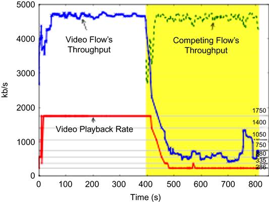
The scenario in which HAS and TCP streams share a bottleneck link is very common in current networks, and hence it is very important to investigate how they share the available bandwidth. This issue was investigated in detail by Huang et al. [24], who carried out a measurement-based study. Their main finding was that HAS streams suffer from what they called a “downward spiral” effect in the presence of a competing TCP flow. This is illustrated in Figure 6.19, in which the TCP flow is introduced a few minutes after the HAS flow starts up. As soon as this happens, the HAS client picks a video rate that is far below the available bandwidth even though both types of flows share the same round trip latency.
Huang et al. [24] pinpointed the cause of the video rate reduction to step 1 of the ABR algorithm (see Section 6.4), during which the receiver estimates the TCP throughput of the video stream using equation 3). If the computed throughput is an underestimation of the actual available bandwidth, then this can lead to the “downward spiral” shown in Figure 6.19. This indeed turns out to be the case, and the detailed dynamics are as follows:
The following scenario assumes a bottleneck rate of 2.5 mbps.
• In the absence of the competing TCP flow, the HAS stream settles into the usual ON-OFF sequence. During the OFF period, the TCP congestion window times out because of inactivity of greater than 200 ms and resets cwnd to the initial value of 10 packets. Hence, the sender needs to ramp up from slow-start for each new chunk.
• When the competing TCP flow is started, then it fills up the buffer at the bottleneck node during the time the video flow is in its OFF period. As a result, when the video flow turns ON again, it experiences a high packet loss, which results in a decrease in its TCP window size. Also, the chunk transmission finishes before the video streams TCP window has a chance to recover.
• As a result because the ABR estimate of the video rate in equation 7, is actually an estimate of the TCP flow on which the video is riding, and because the TCP throughput suffers in the presence of a competing flow because of the reasons explained earlier, it follows that the ABR algorithm badly underestimates the available link bandwidth.
6.8 Further Reading
The YouTube video service from Google does not make use of HAS [25,26]. Instead, it uses a modified form of TCP-based Progressive Download (PD) to transmit the video stream, which operates as follows: At startup, the server transmits the video as fast as it can until the playout buffer (which is 40 sec in size) at the receiver is full. Then it uses rate control to space out the rest of the video transmission, which is also sent in chunks. If the TCP throughput falls, then the send buffer at the server starts to fill up (see Figure 6.2), and this information is used to backpressure the video server.