Keywords

Project Remy; Remy congestion control algorithm; Machine Learning and congestion control; Software Defined Networking and congestion control; Google Congestion Control; GCC; Kalman filtering and congestion control

9.1 Introduction

In this chapter, our objective is to provide a brief survey of some emerging topics in congestion control. There has been renewed interest in the topic of congestion control in recent years, driven mostly by applications to data center networks and video streaming. Meanwhile, broader trends in networking, such as the emergence of Software Defined Networks (SDNs), are beginning to have their influence felt on this topic as well. Other advances in technology, such as the progress that has been made in artificial intelligence (AI) and Machine Learning (ML) algorithms, are also having an impact on our subject.

In Section 9.2, we describe Project Remy from Massachusetts Institute of Technology (MIT), which uses ML to automatically generate congestion control algorithms; these have been shown to perform better than their human-designed counterparts. These algorithms are based on the theory developed in Chapter 3 in which congestion control rules are derived as a solution to a distributed optimization problem. Unlike the window increase–decrease rules that we have encountered so far, these rules number in the hundreds and are a function of the specific point in the feedback space. The framework of Project Remy also helps us to explore the delay versus throughput tradeoff in congestion control, as well as provide bounds on how well the best performing algorithm can do.

In Section 9.3, we give a brief description of the field of SDNs. They have been used to facilitate routing and switching level functionality, but they may have a significant impact on congestion control as well. We describe a couple of topics in congestion control that can benefit from the centralized control point that SDNs provide. The first topic is on the use of SDNs to choose an appropriate Active Queue Management (AQM) algorithm at a switch as a function of the application running on top of the connection. For example, drop-tail queues are good enough for applications that prioritize throughput over latency, but more sophisticated AQM is needed for applications for which low latency is important. The second topic is on the use of SDNs to set appropriate parameters for the AQM algorithm.

Section 9.4 is on the Google Congestion Control (GCC) algorithm, which was designed for transmitting real-time video streams and is part of the Web Real-Time Communication (WebRTC) project of the Internet Engineering Task Force (IETF). There are some interesting new ideas in GCC, such as the active participation of the receiver in the congestion control algorithm, which are sure to influence the future direction of this subject. The GCC algorithm does not run on top of TCP but instead uses the Real Time Transport protocol (RTP) for sending data and its accompanying Real Time Control Protocol (RTCP) for obtaining feedback from the receiver. The receiver analyzes the pattern of packet inter-arrival times and then uses a Kalman filter to estimate whether the bottleneck queue is changing in size. It chooses a rate based on this information and feeds this information back to the source, which bases the sending rate on this and some other pieces of information.

9.2 Machine Learning and Congestion Control: Project Remy

In this section, we describe the work carried out by Winstein et al. at MIT in which they did a fundamental rethink on how to solve the congestion control problem, based on which they came up with an algorithm called Remy that is radically different from all existing work in this area [1–4]. This algorithm is based on applying ideas from partially observable Markov decision processes (POMDPs) to the congestion control problem.

The basic idea behind the derivation of this algorithm is something that we discovered in Chapter 3, that is, the congestion control problem can be regarded as the solution to the distributed optimization of a network wide utility function (see Section 3.2 and Appendix 3.E in Chapter 3). By using POMDP/ML techniques, the algorithm learns the best possible congestion control action, in the sense of minimizing this utility function, based on its observations of the partial network state at each source.

The system uses a simple ON-OFF model for the traffic generation process at each source. The sender is OFF for a duration that is drawn from an exponential distribution. Then it switches to the ON state, where it generates a certain number of bytes that are drawn from an empirical distribution of flow sizes or a closed form distribution.

The important ingredients that go into the algorithm include:

We describe each of these in turn:

1. Utility function: Define the function

$U_{\alpha }(x)=\frac{x^{1-\alpha }}{1-\alpha }$ (1)

(1)

then the form of the network utility function for a connection that Remy uses is given by

$U_{\alpha \beta \delta }(r,T_s)=U_{\alpha }(r)-\delta U_{\beta }(T_s)$ (2)

(2)

Given a network trace, r is estimated as the average throughput for the connection (total number of bytes sent divided by the total time that the connection was “ON”), and T_s is estimated as the average round-trip delay. Note that the parameters $\alpha$ and $\beta$ express the fairness vs efficiency tradeoffs for the throughput and delay, respectively (see Appendix 3.E in Chapter 3), and $\delta$ expresses the relative importance of delay versus throughput. By varying the parameter $\delta$, equation 2 enables us to explicitly control the trade-off between throughput and delay for the algorithm. The reader may recall from the section on Controlled Delay (CoDel) in Chapter 4 that legacy protocols such as Reno or Cubic try to maximize the throughput without worrying about the end-to-end latency. To realize the throughput–delay tradeoff, legacy protocols have to use an AQM such as Random Early Detection (RED) or CoDel, which sacrifice some the throughput to achieve a lower delay. Remy, on the other hand, with the help of the utility function in equation 2, is able to attain this trade-off without making use of an in-network AQM scheme.

2. Network state observations: Remy tracks the following features of the network history, which are updated every time it receives an ACK:

a. ack_ewma: This is an exponentially weighted moving average of the inter-arrival time between new ACKs received, where each new sample contributes 1/8 of the weight of the moving average.

b. send_ewma: This is an exponentially weighted moving average of the time between TCP sender timestamps reflected in those ACKs, with the same weight 1/8 for new samples.

c. rtt_ratio: This is the ratio between the most recent Round Trip Latency (RTT) and the minimum RTT seen during the current connection.

Winstein et al. [3] arrived at this set of observations by doing a comprehensive test of other types of feedback measurements that are possible at a source. Traditional measurements, such as most recent RTT sample or a smoothed estimate of the RTT sample, were tested and discarded because it was observed that they did not improve the performance of the resulting protocol. In particular, Remy does not make use of two variables that almost every other TCP algorithm uses: the packet drop rate p and the round trip latency T. The packet drop rate is not used because a well-functioning algorithm should naturally lead to networks with small queues and very few losses. The round trip latency T was intentionally kept out because the designers did not want the algorithm to take T into account in figuring out the optimal action to take.

Note that Remy does not keep memory from one busy period to the next at a source, so that all the estimates are reset every time a busy period starts.

Hence, in addition to the traditional multiplicative decrease/additive decrease actions, Remy implements a combination of window+rate-based transmission policy, where the interval between transmissions does not exceed $\tau$ seconds.

At a high level, Remy Congestion Control (RemyCC) consists of a set of piecewise constant rules, called the Rule Table, where each rule maps a rectangular region of the observation space to a three dimensional action. On receiving an ACK, RemyCC updates its values for (ack_ewma, send_ewma, rtt_ratio) and then executes the corresponding action (b, a, $\tau$).

We now describe how these rules are generated:

Remy randomly generates millions of different network configurations by picking up random values (within a range) for the link rates, delays, the number of connections, and the on-off traffic distributions for the connections. At each evaluation step, 16 to 100 sample networks are drawn and then simulated for an extended period of time using the RemyCC algorithm. At the end of the simulation, the objective function given by equation 2 is evaluated by summing up the contribution from each connection to produce a network-wide number. The following two special cases were considered:

$U=\log R-\delta \log T,$ (3)

(3)

corresponding to proportional throughput and delay fairness and

$U=-\frac{1}{R}$ (4)

(4)

which corresponds to minimizing the potential delay of a fixed-length transfer.

RemyCC is initialized with the following default rule that applies to all states: b=1, a=1, $\tau =0.01$. This means that initially there is a single cube that contains all the states. Each entry in the rule table has an “epoch,” and Remy maintains a global epoch number initialized to zero.

The following offline automated design procedure is used to come up with the rule table:

If any of the candidate actions lead to an improvement, then replace the original action by the improved action and repeat the search, with the same set of networks and random seed. Otherwise, increment the epoch number of the current rule and go back to step 2. At the first iteration, this will result in the legacy additive increase/multiplicative decrease (AIMD)–type algorithm because the value of the parameters a, b are the same for every state.

An application of this algorithm results in a process whereby areas of the state space that are more likely to occur receive more attention from the optimizer and get subdivided into smaller cubes, thus leading to a more granular action.

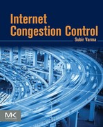
Figure 9.1 shows the results of a comparison of TCP Remy with legacy congestion control protocols (the figure plots the throughput averaged over all sources on the y-axis and the average queuing delay at the bottleneck on the x-axis). A 15-mbps dumbbell topology with a round trip of 150 ms and n=8 connections was used, with each source alternating between a busy period that generates an exponentially distributed byte length of 100 Kbytes and an exponentially distributed off time of 0.5 sec. RemyCC is simulated with the utility function in equation 3 and with three different values of $\delta$, with higher values corresponding to more importance given to delay. The RemyCC algorithm that was generated for this system had between 162 and 204 rules.

The results in Figure 9.1 show that RemyCC outperformed all the legacy algorithms, even those that have an AQM component, such as CUBIC over CoDel with stochastic fair queuing. Further experimental results can be found in Winstein [3].

Figure 9.1 also illustrates that existing congestion control algorithms can be classified by their throughput versus delay performance. Algorithms that prioritize delay over throughput, such as Vegas, lie in lower right hand corner, and those that prioritize throughput over delay lie in the upper left-hand part of the graph. The performance numbers for RemyCC trace an outer arc, which corresponds to the best throughput that can be achieved, for a particular value of the delay constraint. Thus, this framework provides a convenient way of measuring the performance of a congestion control algorithm and how close they are to the ideal performance limit.

Because of the complexity of the rules that RemyCC uses, so far the reasons of its superior performance are not well understood and are still being actively investigated.

9.3 Software Defined Networks and Congestion Control

Software Defined Networks were invented with the objective of simplifying and increasing the flexibility of the network control plane (NCP) algorithms such as routing and switching. In general, these algorithms are notoriously difficult to change because they involve the creation and maintenance of a network-wide distributed system model that maintains a current map of the network state and is capable of functioning under uncertain conditions in a wide variety of scenarios. Rather than running an instance of the NCP in every node, as is done in legacy networks, an SDN centralizes this function in a controller node. This leads to a number of benefits as explained below.

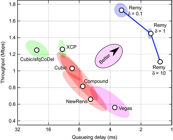
Figure 9.2 shows the basic architecture for an SDN network, which is made up of two principal components, namely OpenFlow-controlled switches and the SDN controller. Note that the NCP located in the controller is centralized and exists separately from the data plane located in the network switches. The controller communicates with the switches using an out-of-band communication network (shown with the dotted line) using the OpenFlow protocol.

The SDN controller can be implemented in software on a standard server platform. It is implemented using a layered architecture, with the bottom layer called the Network Operating System (NOS) and the upper layer consisting of one or more applications, such as routing, that are used to control the OpenFlow switches. The NOS layer is responsible for managing the communications between the controller and the switches. In addition it also responsible for creating and maintaining a current topology map of the network. This topology map is exposed to the applications running in the controller on its northbound interface (Figure 9.2 shows some example applications running in the SDN network, such as Traffic Management (TM), Network Configuration (Config), Packet Forwarding (FW), and Load Balancing (LB)). As a result of this design, every control application shares a common Distributed System, unlike in current networks, where every application needs to implement its own Distributed System (e.g., the network map maintained by Layer 3 protocol such as OSPF is different from that maintained by a Layer 2 protocol such as Spanning Tree). Moreover, the problem of designing a distributed control algorithm is reduced to a pure software problem because the control algorithm can operate on the network abstraction created by the NOS rather than the real network.

Even though most of the initial work in SDNs has gone into the investigation of its impact on the NCP, researchers have begun to investigate ways in which it might be used to improve the operation of the data plane as well. We describe a couple of ways in which this can be done in Sections 3.1 and 3.2.

9.3.1 Using Software Defined Networks to Choose Active Queue Management Algorithms on a Per-Application Basis

In the discussion of the CoDel AQM algorithm in Chapter 4, we first introduced the notion that the most appropriate AQM algorithm is a function of the application, and this line of reasoning is developed further here. In general, based on their performance requirements, applications fall into the following three categories:

1. Throughput maximization: Applications in this category, such as File Transfer Protocol (FTP), are only interested in maximizing their data throughput, regardless of the latency.

2. Power maximization: Recall that the power of a connection was defined as a function of the average throughput R_av, and average latency T_s as

$Power=\frac{R_{av}}{T_s}$ (5)

(5)

Applications such as video conferencing are interested in achieving a high throughput, but at the same time, they like to keep their latencies low. Hence, they belong to the power maximization category.

3. Minimization of Flow Completion Time (FCT): Web surfing (or HTTP transfer) is a typical application in this category, in which the transfer size is smaller compared with FTPs and the user is interested in minimizing the total time needed to complete a page download.

Note that throughput maximization for a connection also leads to FCT minimization; hence, the first and third categories are related. In the context of a network where both types of connections pass through a common link, the presence of the FTP connection can severely downgrade the FCT of a web page download if they both share a buffer at the bottleneck node. Ways in which this problem can be avoided are:

a. By using an AQM scheme such as CoDel to control the queue size at the bottleneck node: CoDel will keep the buffer occupancy and hence the latency low but at the expense of a reduction in the throughput in both the FTP and HTTP connection. This is not an ideal situation because the FTP connection has to give up some of its throughput to keep the latency for the HTTP connection down.

b. By isolating the FTP and HTTP connections at the bottleneck node into their own subqueues, by using a queue scheduling algorithm such as Fair Queuing: In this case, neither subqueue requires an AQM controller. The HTTP connection will only see the contribution to its latency caused by its own queue, which will keep it low, and the FTP connection can maintain a large subqueue at the bottleneck to keep its throughput up without having to worry about the latency. This is clearly a better solution than a).

If an FTP and video conferencing flow (as representatives of categories 1 and 2) share a bottleneck node buffer, then again we run into the same problem, that is, the queuing delay attributable to the FTP will degrade the video conferencing session. Again, we can use an AQM scheme at the node to keep the queuing delay low, but this will be at a cost of decrease in FTP throughput of 50% or more (see Sivaraman et al. [5]). A better solution would be to isolate the two flows using Fair Queuing and then use an AQM scheme such as CoDel only on the video conferencing connection.

From this discussion, it follows that the most appropriate AQM scheme at a node is a function of the application that is running on top of the TCP connection. By using fair queuing, a node can isolate each connection into its own subqueue and then apply a (potentially) different AQM scheme to each subqueue. Sivaraman et al. [5] propose that this allocation of an AQM algorithm to a connection can be done using the SDN infrastructure. Hence, the SDN controller can match the type of application using the TCP connection to the most appropriate AQM algorithm at each node that the connection passes through. Using the OpenFlow protocol, it can then configure the queue management logic to the selected algorithm.

The capability of dynamically reconfiguring the AQM algorithm at a switch does not currently exist in the current generation of switches and routers. These are somewhat inflexible because the queue management logic is implemented in hardware to be able to function at high speeds. Sivaraman et al. [5] propose that the queue management logic be implemented in an Field Programmable Gate Array (FPGA), so that it can be reconfigured by the SDN controller. They actually implemented the CoDel and RED AQM algorithms in a Xilinx FPGA, which was able to support a link speed of 10 Gbps, to show the feasibility of this approach. The other hurdle in implementing this system is that currently there is no way for applications to signal their performance requirements to the SDN controller.

9.3.2 Using Software Defined Networks to Adapt Random Early Detection Parameters

Recall from the analysis in Chapter 3 that a RED algorithm is stable (in the sense of not causing large queue fluctuations) for number of connections greater than N⁻ and round trip latency less than T⁺, if the following conditions are satisfied:

$\frac{L_{red}{(T^{+}C)}^3}{{(2N^{-})}^2}\le \sqrt{\frac{{\omega }_c^2}{K^2}+1}\mathrm{where}$ (6)

(6)

${\omega }_c=0.1\min \left\{\frac{2N^{-}}{{(T^{+})}^{2}C},\frac{1}{T^{+}}\right\},L_{red}=\frac{{\max }_p}{{\max }_{th}-{\min }_{th}},K=-\frac{{\log }_e(1-w_q)}{\delta }$

Hence, a RED algorithm can become unstable if

• The number of connections passing through the link becomes too small, or

• The round trip latency for the connection becomes too big, or

• The link capacity becomes too large.

One way in which instability can be avoided was described in Chapter 4, which is by using the Adaptive RED (ARED) algorithm that changes the parameter max_p as a function of the observed queue size at the node. We propose that another way of adapting RED is by making direct use of equation 6 and using the SDN controller to change RED parameters as the link conditions change.

Note that the number of connections N and the link capacity C are the two link parameters that influence the stability condition (equation 6), and the end-to-end latency T is a property of the connection path. As explained in Chapter 4, C is subject to large fluctuations in cellular wireless links; however, it may not be possible to do real-time monitoring of this quantity from the SDN controller. On the other hand, for wireline connections, C is fixed, and the only variables are N and T, which change relatively slowly. Moreover, the SDN controller tracks all active connections in the network as part of its base function, and hence it can easily figure out the number of active connections passing through each node. The round trip latency can be reported by applications to the SDN controller using a yet to be defined interface between the two.

Using these two pieces of information, the SDN controller can then use equation 6 to compute the values of L_red and K to achieve stability and thereby set the RED parameters max_p, max_th, min_th, and w_q. Following ARED, it can choose to vary only max_p while keeping the other parameters fixed, but it has more flexibility in this regard.

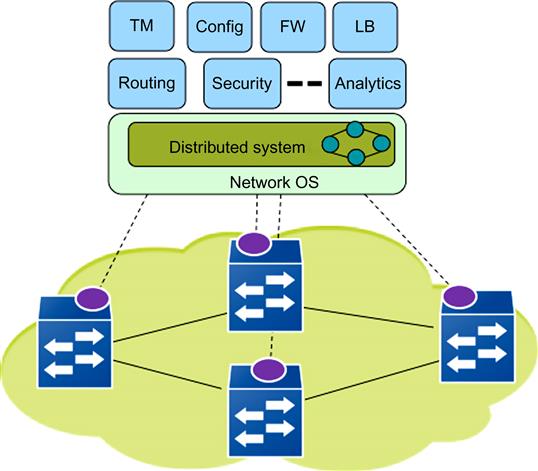
Another example of this is the use of the equation

${\tau }^{*}\approx \frac{{\tan }^{-1}\left[{\displaystyle \frac{G_d{w}^2}{N{p}_s}}\sqrt{0.5+\sqrt{0.25+{\left({\displaystyle \frac{N{p}_s}{G_d{w}^2}}\right)}^2}}\right]}{{\displaystyle \frac{G_{d}wC}{N}}\sqrt{0.5+\sqrt{0.25+{\left({\displaystyle \frac{N{p}_s}{G_d{w}^2}}\right)}^2}}}$

which gives the stability threshold for the QCN algorithm in Ethernet networks as a function of the link speed C, number of connections N and algorithm parameters (p_s, w, G_d) (see Chapter 8, Section 8.5). As the number of connections N varies, the SDN controller can vary the algorithm parameters to maintain the stability threshold in the desired range.

9.4 The Google Congestion Control (GCC) Algorithm

The GCC algorithm [6,7] belongs to the category of congestion control algorithms that are used for real-time streams such as telephony and video conferencing. Delivery of real-time media is actually a fairly large subcategory in itself that is characterized the by following:

The information in the RTCP RR report is then used by the source to control its transmission rate. Traditionally, the TCP Friendly Rate Control Algorithm (TFRC) has been used for this purpose (see Floyd et al. [8] for a description of TFRC). This algorithm controls the transmit rate as a function of the loss event rate statistic that is reported by the receiver.

There are a number of problems in using TFRC in modern cellular networks, including:

The GCC algorithm is designed to address these shortcomings. It is part of the RTCWeb project within the IETF, which also includes other specifications to enable real-time audio and video communication within web browsers without the need for installing any plug-in or additional third-party software. GCC is available in the latest versions of the web browser Google Chrome.

The GCC algorithm tries to fully use the bottleneck link while keeping the queuing delay small. We came across the problem of minimizing queuing delays on a variable capacity link in the context of TCP in Chapter 4, where the solutions included using AQM techniques such as CoDel or end-to-end algorithms such as Low Extra Delay Background Transport (LEDBAT). The GCC algorithm belongs to the latter category since it does not require any AQM at the intermediate nodes. (Note that LEDBAT is not directly applicable here because it relies on the regular flow of TCP ACKs for feedback.) GCC uses a sophisticated technique using Kalman filters to figure out if the bottleneck queue is increasing or decreasing and uses this information to compute a number called the Receive Rate. It sends the Receive Rate back to the source in a special control packet called REMB, which then combines it with other information such as the packet loss rate to determine the final transmit rate.

The GCC algorithm is composed of two modules, one of which runs at the sender and the other at the receiver. These are described in the next two sections.

9.4.1 Sender Side Rate Computation

The sender combines several pieces of information to come up with the transmit rate, including the packet loss rate (as conveyed by the RTCP RR packets), the rate of an equivalent TFRC source, and the rates coming from the receiver in the REMB packets.

Define the following:

t_k: Arrival time of the k^th RTCP RR packet

t_r: Arrival time of the r^th REMB packet

R_s(t_k): Sender transmit rate at time t=t_k

R_r(t_r): Receiver computed rate in the REMB message received t=t_r

X(t_k): Sending rate as computed using the TFRC algorithm at time t=t_k

f_l(t_k): Fraction of lost packets at t=t_k

On receipt of the k^th RTCP RR packet, the sender uses the following formula to compute its rate:

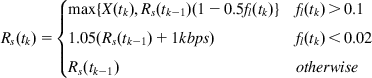$R_s(t_k)=\{\begin{array}{ll}\max \{X(t_k),R_s(t_{k-1})(1-0.5f_l(t_k)\}\hfill & f_l(t_k)>0.1\hfill \\ 1.05(R_s(t_{k-1})+1kbps)\hfill & f_l(t_k)<0.02\hfill \\ R_s(t_{k-1})\hfill & otherwise\hfill \end{array}$ (7)

(7)

The reasoning behind these rules is the following:

• When the fraction of lost packets exceeds 10%, then the rate is multiplicatively decreased but not below the equivalent TFRC rate.

• When the fraction of lost packets is less than 2%, then the rate is multiplicatively increased.

• When the packet loss rate is between 2% and 10%, then the rate is kept constant.

Hence, in contrast to TCP, the GCC sender does not decrease its rate even for loss rates as high as 10%, and actually increases the rate for loss rates under 2%. This is done because video streams are capable of hiding the artifacts created because of smaller packet loss rates.

When the sender receives the r^th REMB packet, it modifies its sending rate as per the following equation:

$R_s(t_r)\leftarrow \min \{R_s(t_r),R_r(t_r)\}$ (8)

(8)

9.4.2 Receiver Side Rate Computation

The novelty of the GCC algorithm lies in its receiver side rate computation algorithm. By filtering the stream of received packets, it tries to detect variations in the bottleneck queue size and uses this information to set the receive rate. It can be decomposed into three parts: an arrival time filter, an overuse detector, and a remote rate control.

9.4.2.1 Arrival Time Model and Filter

In the RTCWeb protocol, packets are grouped into frames, such that all packets in a frame share the same timestamp.

Define the following:

t_i: Time when all the packets in the i^th frame have been received

${\tau }_i$: RTP timestamp for the i^th frame

L(t_i): Size of the i^th frame

C(t_i): Estimate of the bottleneck link capacity at t=t_i

b(t_i): Queuing time variation at t=t_i

Note that a frame is delayed relative to its predecessor if $t_i-{\tau }_i>t_{i-1}-{\tau }_{i-1}$. We define the sequence d_i to be the difference between these two sequences, so that

$d_i=t_i-t_{i-1}-({\tau }_i-{\tau }_{i-1})$ (9)

(9)

Variations in d_i can be caused by the following factors: (1) changes in the bottleneck link capacity C, (2) changes in the size of the video frame L, (3) changes in bottleneck queue size b, or (4) network jitter. All of these factors are captured in the following model for d_i:

$d_i=\frac{L(t_i)-L(t_{i-1})}{C(t_i)}+b(t_i)+n(t_i)$ (10)

(10)

Note that the network jitter process n(t_i) has zero mean because the drift in queue size is captured in the previous term b(t_i).

Using equation 10, GCC uses a Kalman filter (see Appendix 9.A) to obtain estimates of the sequences C(t_i) and b(t_i) and then uses these values to find out if the bottleneck queue is oversubscribed (the queue length is increasing) or undersubscribed. The calculations are as follows:

Define ${\xi }_i={[1/C(t_i)b(t_i)]}^T$ as the “hidden” state of the system, which obeys the following state evolution equation:

${\xi }_{i+1}={\xi }_i+u_i$ (11)

(11)

where u_i is a white Gaussian noise process with zero mean and covariance Q_i.

From equation 10, it follows that the observation process d_i obeys the following equation

$d_i=h_i{\xi }_i+v_i$ (12)

(12)

where $h_i=[L(t_i)-L(t_{i-1})1]$ and v_i is a white Gaussian noise process with zero mean and variance S_i.

Let ${\hat{\xi }}_i={[1/\hat{C}(t_i)\hat{b}(t_i)]}^T$ be the sequence representing the estimate for ${\xi }_i$. From Kalman filtering theory, it follows that

${\hat{\xi }}_i={\hat{\xi }}_{i-1}+K_i(d_i-h_i{\hat{\xi }}_{i-1})$ (13)

(13)

where K_i is the Kalman gain given by

$K_i=\frac{E_{i-1}{h}_i^T}{{\hat{S}}_i+h_i{E}_{i-1}{h}_i^T}and{E}_i=(I-K_i{h}_i)E_{i-1}+Q_i$ (14)

(14)

The variance S_i is estimated using an exponential averaging filter modified for variable sampling rate, as

${\hat{S}}_i^2=\beta {\hat{S}}_{i-1}^2+(1-\beta ){(d_i-h_i{\hat{\xi }}_{i-1})}^2\mathrm{and}$

$\beta ={(1-\alpha )}^{\frac{30}{1000f_{\max }}}where{f}_{\max }=\max \left\{\frac{1}{{\tau }_j-{\tau }_{j-1}}\right\}\mathrm{for}$

$j=i-K+1,\dots ,i\alpha \in [0.1,0.001]$

Q_i is chosen to be a diagonal matrix with the main diagonal elements given by

$diag(Q(i))=\frac{30}{1000f_{\max }}{\left[{10}^{-10}{10}^{-2}\right]}^T.$

These filter parameters are scaled with the frame rate to make the detector respond as quickly to low frame rates as at high frame rates.

9.4.2.2 Remote Rate Control

Assuming that the last packet in the i^th frame is received at time t_i, the receiver computes the rate R_r(t_i) according to the following formula:

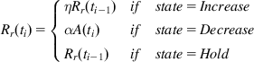$R_r(t_i)=\{\begin{array}{lll}\eta R_r(t_{i-1})\hfill & if\hfill & state=Increase\hfill \\ \alpha A(t_i)\hfill & if\hfill & state=Decrease\hfill \\ R_r(t_{i-1})\hfill & if\hfill & state=Hold\hfill \end{array}$ (15)

(15)

where $\eta \in [1.005,1.3]$, $\alpha \in [0.8,0.95]$ and A(t_i) is the receiving rate measured in the last 500 ms. Also, the R_r(t_i) cannot exceed 1.5*A(t_i) in order to prevent the receiver from requesting a bitrate that the sender cannot satisfy.

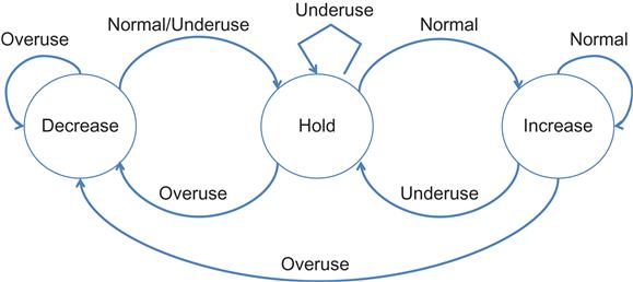
Note that the rates are controlled by the state of the Finite State Machine (FSM) in Figure 9.3, which is called the Remote Rate Controller. The state of this FSM is changed according to the signal produced by the Overuse Detector, which is based on the output of the Arrival Time Filter, as follows:

• If $\hat{b}(t_i)$ increases above a threshold and keeps increasing for a certain amount of time or for a certain amount of consecutive frames, it is assumed that the network is congested because the bottleneck queue is filling up, and the “overuse” signal is triggered.

• If $\hat{b}(t_i)$ decreases below a threshold, this means that the bottleneck queue is being emptied. Hence, the network is considered underused, and the “underuse” signal is generated. Upon this signal, the FSM enters the Hold state, where the available bandwidth estimate is held constant while waiting for the queues to stabilize at a lower level.

• When $\hat{b}(t_i)$ is close to zero, the network is considered stable, and the “normal” signal is generated.

The REMB messages that carry the value of R_r from the receiver to the sender are sent either every 1 sec if R_r is decreasing or immediately if R_r decreases more than 3%.

Appendix 9.A Kalman Filtering

Consider a linear system, with an n×1 dimensional state variable x_t, which evolves in time according to the following equation:

$x_t=A_t{x}_{t-1}+B_t{u}_t+{\epsilon }_t$ (F1)

(F1)

where u_t is a m×1 dimensional control vector driving x_t, A_t is a square matrix of size n×n, B_t is n×m matrix, and ${\epsilon }_t$ is a n×1 Gaussian random vector with mean 0 and covariance given by R_t. A state transition of the type (F1) is known as linear Gaussian to reflect the fact that it is linear in its arguments with additive Gaussian noise.

The system state x_t is not observable directly; its value has to be inferred through the k×1 dimensional state observation process z_t given by

$z_t=C_t{x}_t+{\delta }_t$ (F2)

(F2)

where C_t is k×n dimensional matrix and ${\delta }_t$ is the observation (or measurement) noise process. The distribution of ${\delta }_t$ is assumed to be multivariate Gaussian with zero mean and covariance Q_t.

The Kalman filter is used to obtain estimates of the state variable x_t at time t, given the control sequence u_t and output sequence z_t. Because x_t is a Gaussian random variable, the estimates are actually estimates for its mean ${\mu }_t$ and covariance ${\mathrm{\Sigma }}_t$ at time t.

The Kalman filter uses an iterative scheme, which works as follows:

1. At time t=0, start with initial estimates for the mean and covariance of x_t given by $({\mu }_0,{\mathrm{\Sigma }}_0)$.

2. At time t–1, assume that the estimates for the mean and covariance of x_t−1 have been computed to be $({\mu }_{t-1},{\mathrm{\Sigma }}_{t-1})$. Given the control u_t and output z_t at time t, the estimates $({\mu }_t,{\mathrm{\Sigma }}_t)$ are computed recursively as follows, in two steps.

3. In step a, the control u_t is incorporated (but not the measurement z_t), to obtain the intermediate estimates $({\overline{\mu }}_t,{\overline{\mathrm{\Sigma }}}_t)$ given by

${\overline{\mu }}_t=A_t{\mu }_{t-1}+B_t{u}_t$ (F3)

(F3)

${\overline{\Sigma }}_t=A_t{\Sigma }_{t-1}{A}_t^T+R_t$ (F4)

(F4)

4. In step b, the measurement z_t is incorporated to obtain the estimates $({\mu }_t,{\mathrm{\Sigma }}_t)$ at time t, given by

$K_t={{\displaystyle \overline{\mathrm{\Sigma }}}}_t{C}_t^T{(C_t{\overline{\mathrm{\Sigma }}}_t{C}_t^T+Q_t)}^{-1}$ (F5)

(F5)

${\mu }_t={\overline{\mu }}_t+K_t(z_t-C_t{\overline{\mu }}_t)$ (F6)

(F6)

${\mathrm{\Sigma }}_t=(I-K_t{C}_t){\overline{\mathrm{\Sigma }}}_t$ (F7)

(F7)

The variable K_t computed in equation F6 is called the Kalman gain, and it specifies the degree to which the new measurement is incorporated into the new state estimate.