Graph algorithms on GPUs
F. Busato; N. Bombieri University of Verona, Verona, Italy
Abstract
This chapter introduces the topic of graph algorithms on graphics processing units (GPUs). It starts by presenting and comparing the most important data structures and techniques applied for representing and analyzing graphs on state-of-the-art GPUs. It then presents the theory and an updated review of the most efficient implementations of graph algorithms for GPUs. In particular, the chapter focuses on graph traversal algorithms (breadth-first search), single-source shortest path (Djikstra, Bellman-Ford, delta stepping, hybrids), and all-pairs shortest path (Floyd-Warshall). By the end of the chapter, load balancing and memory access techniques are discussed through an overview of their main issues and management techniques.
Keywords
Graph algorithms; BFS; SSSP; APSP; Load balancing
1 Graph representation for GPUs
The graph representation adopted when implementing a graph algorithm for graphics processing units (GPUs) strongly affects implementation efficiency and performance. The three most common representations are adjacency matrices, adjacency lists, and egdes lists [1, 2]. They have different characteristics and each one finds the best application in different contexts (i.e., graph and algorithm characteristics).
As for the sequential implementations, the quality and efficiency of the graph representation can be measured over three properties: the involved memory footprint, the time required to determine whether a given edge is in the graph, and the time it takes to find the neighbors of a given vertex. For GPU implementations, such a measure also involves load balancing and the memory coalescing.
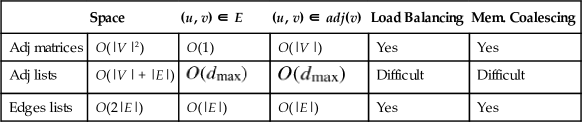
Given a graph G = (V, E), where V is the set of vertices, E is the set of edges, and ![]() is the largest diameter of the graph, Table 1 summarizes the main features of the data representations, which are discussed in detail in the next paragraphs.
is the largest diameter of the graph, Table 1 summarizes the main features of the data representations, which are discussed in detail in the next paragraphs.
Table 1
Main Feature of Data Representations
| Space | (u, v) ∈ E | (u, v) ∈ adj(v) | Load Balancing | Mem. Coalescing | |
| Adj matrices | O(|V |2) | O(1) | O(|V |) | Yes | Yes |
| Adj lists | O(|V | + |E|) | Difficult | Difficult | ||
| Edges lists | O(2|E|) | O(|E|) | O(|E|) | Yes | Yes |
1.1 Adjacency Matrices
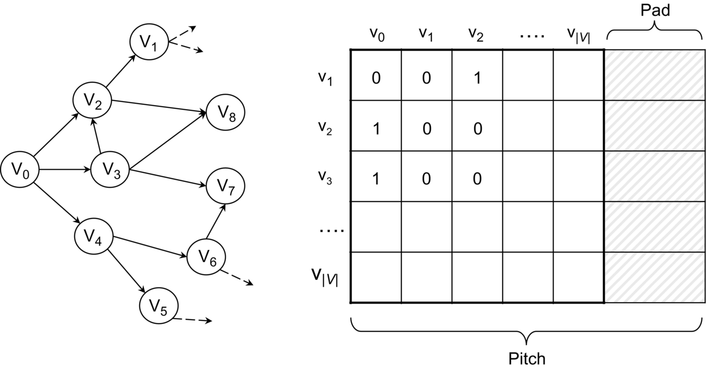
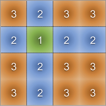
An adjacency matrix allows representing a graph with a V × V matrix M = [f(i, j)] where each element f(i, j) contains the attributes of the edge (i, j). If the edges do not have an attribute, the graph can be represented by a boolean matrix to save memory space (Fig. 1).
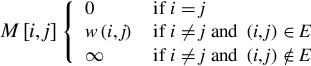
Common algorithms that use this representation are all-pair shortest path (APSP) and transitive closure [3–9]. If the graph is weighted, each value of f(i, j) is defined as follows:
On GPUs, both directed and undirected graphs represented by an adjacency matrix take O(|V |2) memory space, because the whole matrix is stored in memory with a large continuous array. In GPU architectures, it is also important, for performance, to align the matrix with memory to improve coalescence of memory accesses. In this context, the Compute Unified Device Architecture (CUDA) language provides the function cudaMallocPitch [10] to pad the data allocation, with the aim of meeting the alignment requirements for memory coalescing. In this case the indexing changes are as follows:
The O(|V |2) memory space required is the main limitation of the adjacency matrices. Even on recent GPUs, they allow handling of fairly small graphs. For example, on a GPU device with 4 GB of DRAM, graphs that can be represented through an adjacency matrix can have a maximum of only 32,768 vertices (which, for actual graph datasets, is considered restrictive). In general, adjacency matrices best represent small and dense graphs (i.e., |E|≈|V |2). In some cases, such as for the all-pairs shortest path problem, graphs larger than the GPU memory are partitioned and each part is processed independently [7–9].
1.2 Adjacency Lists
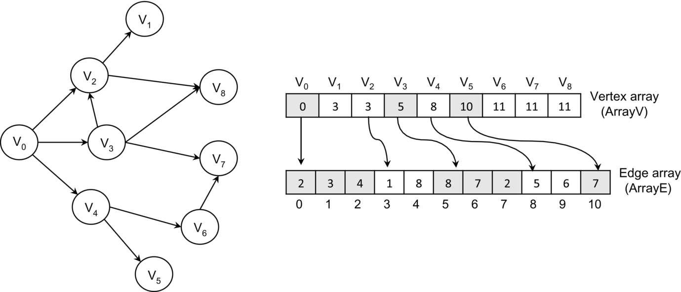
Adjacency lists are the most common representation for sparse graphs, where the number of edges is typically a constant factor larger than |V |. Because the sequential implementation of adjacency lists relies on pointers, they are not suitable for GPUs. They are replaced, in GPU implementations, by the compressed sparse row (CSR) or the compressed row storage (CRS) sparse matrix format [11, 12].
In general, an adjacency list consists of an array of vertices (ArrayV) and an array of edges (ArrayE), where each element in the vertex array stores the starting index (in the edge array) of the edges outgoing from each node. The edge array stores the destination vertices of each edge (Fig. 2). This allows visiting the neighbors of a vertex v by reading the edge array from ArrayV[v] to ArrayV[v + 1].
The attributes of the edges are in general stored in the edge array through an array of structures (AoS). For example, in a weighted graph, the destination and the weight of an edge can be stored in a structure with two integer values (int2 in CUDA [13]). Such a data organization allows many scattered memory accesses to be avoided and, as a consequence, the algorithm performance to be improved.
Undirected graphs represented with the CSR format take O(|V | + 2|E|) space since each edge is stored twice. If the problem also requires the incoming edges, the same format is used to store the reverse graph where the vertex array stores the offsets of the incoming edges. The space required with the reverse graph is O(2|V | + 2|E|).
The main issues of the CSR format are load balancing and memory coalescing because of the irregular structure of such a format. If the algorithm involves visiting each vertex at each iteration, the memory coalescing for the vertex array is simple to achieve, but on the other hand, it is difficult to achieve for the edge array. Achieving both load balancing and memory coalescing requires advanced and sophisticated implementation techniques (see Section 5).
For many graph algorithms, the adjacency list representation guarantees better performance than adjacency matrix and edge lists [14–18].
1.3 Edge Lists
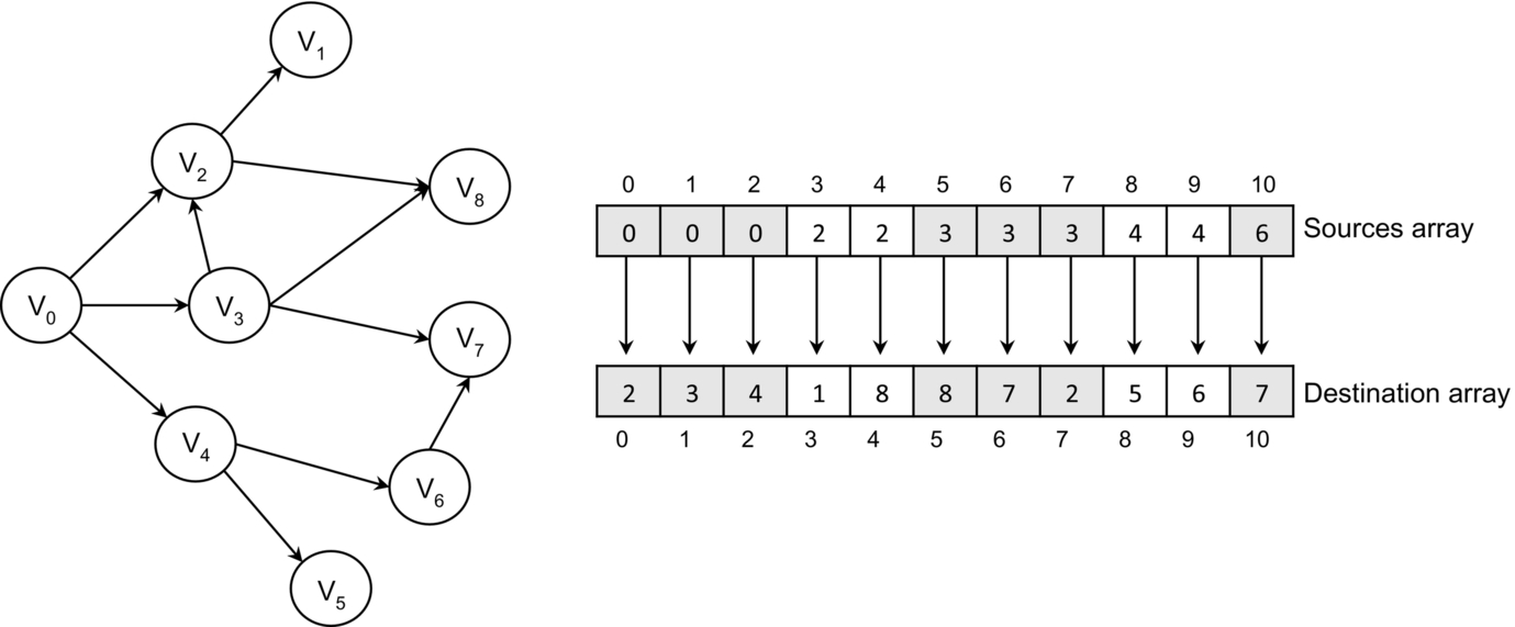
The edge list representation of a graph, also called coordinate list (COO) sparse matrix [19], consists of two arrays of size |E| that store the source and the destination of each edge (Fig. 3). To improve the memory coalescing, similarly to CSR, the source, the destination and other edge attributes (such as the edge weight) can be stored in a single structure (AoS) [20].
Storing some vertex attributes in external arrays is also necessary in many graph algorithms. For this reason, the edge list is sorted by the first vertex in each ordered pair such that adjacent threads are assigned to edges with the same source vertex. This improves coalescence of memory accesses for retrieval of the vertex attributes. In some cases, sorting the edge list in the lexicographic order may also improve coalescence of memory accesses for retrieving the attributes of the destination vertices [21]. The edge organization in a sorted list allows reducing the complexity (from O(|E|) to ![]() ) of verifying whether an edge is in the graph by means of a simple binary search [22].
) of verifying whether an edge is in the graph by means of a simple binary search [22].
For undirected graphs, the edge list should not be replicated for the reverse graph. Processing the incoming edges can be done simply by reading the source-destination pairs in the inverse order, thus halving the number of memory accesses. With this strategy, the space required for the edge list representation is O(2|E|).
The edge list representation is suitable in those algorithms that iterate over all edges. For example, it is used in the GPU implementation of algorithms such as betweenness centrality [21, 23]. In general, this format does not guarantee performance comparable to the adjacency list, but it allows achieving both perfect load balancing and memory coalescing with a simple thread mapping. In graphs with a nonuniform distribution of vertex degrees, the COO format is generally more efficient than CSR [21, 24].
2 Graph traversal algorithms: the breadth first search (BFS)
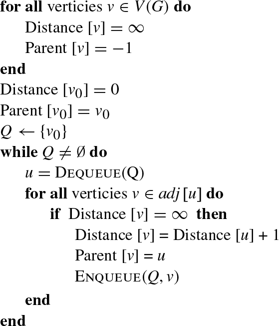
The BFS is a core primitive for graph traversal and the basis for many higher-level graph analysis algorithms. It is used in several different contexts, such as image processing, state space searching, network analysis, graph partitioning, and automatic theorem proving. Given a graph G(V, E), where V is the set of vertices and E is the set of edges, and a source vertex s, the BFS visit inspects every edge of E to find the minimum number of edges or the shortest path to reach every vertex of V from source s. Algorithm 1 summarizes the traditional sequential algorithm [1], where Q is an FIFO queue data structure that stores not-yet-visited vertices, Distance [v] represents the distance of vertex v from the source vertex s (number of edges in the path), and Parent [v] represents the parent vertex of v. An unvisited vertex v is denoted with Distance [v] equal to ![]() . The asymptotic time complexity of the sequential algorithm is O(|V | + |E|).
. The asymptotic time complexity of the sequential algorithm is O(|V | + |E|).
In the context of GPUs, the BFS algorithm is the only graph traversal method applied since it exposes a high level of parallelism. In contrast, the depth-first search traversal is never applied because of its intrinsic sequentiality.
2.1 The Frontier-Based Parallel Implementation of BFS
The most efficient parallel implementations of BFS for GPUs exploit the concept of frontier [1]. They generate a breadth-first tree that has root s and contains all reachable vertices. The vertices in each level of the tree compose a frontier (F). Frontier propagation checks every neighbor of a frontier vertex to see whether it has already been visited. If not, the neighbor is added into a new frontier.
The frontier propagation relies on two data structures, F and F′. F represents the actual frontier, which is read by the parallel threads to start the propagation step. F′ is written by the threads to generate the frontier for the next BFS step. At each step, F′ is filtered and swapped into F for the next iteration. Fig. 4 shows an example, in which starting from vertex “1,” the BFS visit concludes in three steps.1
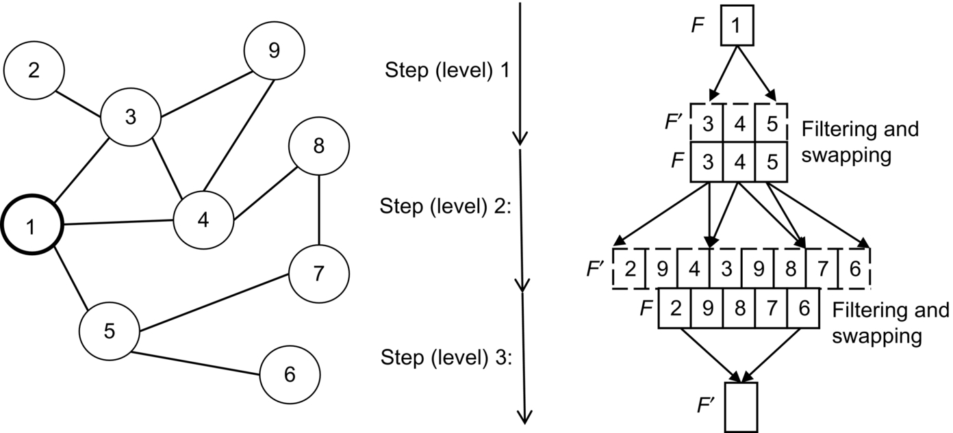
The filtering steps aim at guaranteeing correctness of the BFS visit as well as avoiding useless thread work and waste of resources. When a thread visits a neighbor already visited, that neighbor is eliminated from the frontier (e.g., vertex 3 visited by a thread from vertex 4 in step 2 of Fig. 4). When more threads visit the same neighbor in the same propagation step (e.g., vertex 9 visited by threads 3 and 4 in step 2), they generate duplicate vertices in the frontier. Duplicate vertices cause redundant work in the subsequent propagation steps (i.e., more threads visit the same path) and useless occupancy of shared memory. The most efficient BFS implementations detect and eliminate duplicates by exploiting hash tables, Kepler 8-byte memory access mode, and warp shuffle instructions [15, 16].
Several techniques have been proposed in literature to efficiently parallelize the BFS algorithm for GPUs. Harish and Narayanan [25] proposed the first approach, which relies on exploring all the graph vertices at each iteration (i.e., at each visiting level) to see whether the vertex belongs to the current frontier. This allows the algorithm to save GPU overhead by not maintaining the frontier queues. Nevertheless, the proposed approach on CSR representation, leads to a significant workload imbalance whenever the graph is not homogeneous in terms of vertex degree. In addition, with D as the graph diameter, the computational complexity of such a solution is O(|V ||D| + |E|), where O(|V ||D|) is spent to check the frontier vertices and O(|E|) is spent to explore each graph edge. While this approach fits on dense graphs, in the worst case of sparse graphs (where D = O(|V |)), the algorithm has a complexity of O(|V |2). This implies that, for large graphs, such an implementation is slower than the sequential version.
A partial solution to the problem of workload imbalance was proposed in Ref. [18] by adopting the same graph representation. Instead of assigning a thread to a vertex, the authors propose thread groups (which they call virtual warps) to explore the array of vertices. The group size is typically 2, 4, 8, 16, or 32, and the number of blocks is inversely proportional to the virtual warp size. This leads to a limited speedup in case of low degree graphs, since many threads cannot be exploited at the kernel configuration time. Also, the virtual warp size is static and has to be properly set depending on each graph characteristics.
Ref. [26] presents an alternative solution based on matrices for sparse graphs. Each frontier propagation is transformed into a matrix-vector multiplication. Given the total number of multiplications D (which corresponds to the number of levels), the computational complexity of the algorithm is O(|V | + |E||D|), where O(|V |) is spent to initialize the vector, and O(|E|) is spent for the multiplication at each level. In the worst case, that is, when D = O(|V |), the algorithm complexity is O(|V |2).
Refs. [21, 24] present alternative approaches based on edge parallelism. Instead of assigning one or more threads to a vertex, the thread computation is distributed to edges. As a consequence, the thread divergence is limited, and the workload is balanced even with high-degree graphs. The main drawback is the overhead introduced by the visit of all graph edges at each level. In many cases, the number of edges is much greater than the number of vertices. In these cases, the parallel work is not sufficient to improve the performance against vertex parallelism.
An efficient BFS implementation with computational complexity O(|V | + |E|) is proposed in Ref. [17]. The algorithm exploits a single hierarchical queue shared across all thread blocks and an interblock synchronization [27] to save queue accesses in global memory. Nevertheless, the small frontier size requested to avoid global memory writes and the visit exclusively based on vertex parallelism limit the overall speedup. In addition, the generally high-degree vertices are handled through an expensive precomputation phase rather than at runtime.
Merrill et al. [16] present an algorithm implementation that achieves work complexity O(|V | + |E|). They make use of parallel prefix-scan and three different approaches to deal with the workload imbalance: vertex expansion and edge contraction, edge contraction and vertex expansion, and hybrid. The algorithm also relies on a technique to reduce redundant work because of duplicate vertices on the frontiers.
Beamer et al. propose a central processing unit (CPU) multicore hybrid approach, which combines the frontier-based algorithm along with a bottom-up BFS algorithm. The bottom-up algorithm can greatly reduce the number of edges examined compared to common parallel algorithms. The bottom-up BFS traversal searches vertices of the next iteration (at distance L + 1) in the reverse direction by exploring the unvisted vertices of the graph. This approach requires only a thread per unvisted vertex that explores the neighbor until a previously visited vertex is found (at distance L). The bottom-up BFS is particularly efficient on low-diameter graphs where, at the ending iterations, a substantial fraction of neighbors are valid parents. In the context of GPUs, such a bottom-up approach for graph traversal was implemented by Wang et al. [28] in the Gunrock framework and by Hiragushi et al. [29].
2.2 BFS-4K
BFS-4K [15] is a parallel implementation of BFS for GPUs that exploits the more advanced features of GPU-based platforms (i.e., NVIDIA Kepler, Maxwell [30, 31]) to improve the performance w.r.t. the sequential CPU implementations and to achieve an asymptotically optimal work complexity.
BFS-4K implements different techniques to deal with the potential workload imbalance and thread divergence caused by actual graph nonhomogeneity (e.g., number of vertices, edges, diameter, vertex degree), as follows:
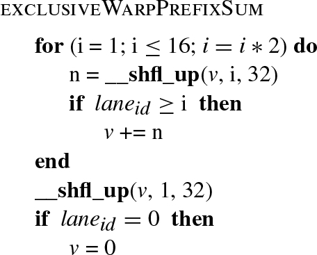
• Exclusive prefix-sum. To improve data access time and thread concurrency during the propagation steps, the frontier data structures are stored in shared memory and handled by a prefix-sum procedure [32, 33]. Such a procedure is implemented through warp shuffle instructions of the Kepler architecture. BFS-4K implements a two-level exclusive prefix-sum, that is, at warp-level and block-level. The first is implemented by using Kepler warp-shuffle instructions, which guarantee the result computation in ![]() steps. Algorithm 2 shows a high-level representation of such a prefix-sum procedure implemented with a warp shuffle instruction (i.e., __shfl_up()).
steps. Algorithm 2 shows a high-level representation of such a prefix-sum procedure implemented with a warp shuffle instruction (i.e., __shfl_up()).
• Dynamic virtual warps. The virtual warp technique presented in Ref. [18] is applied to minimize the waste of GPU resources and to reduce the divergence during the neighbor inspection phase. The idea is to allocate a chunk of tasks to each warp and to execute different tasks as serial rather than assigning a different task to each thread. Multiple threads are used in a warp for explicit single instruction multiple data (SIMD) operations only, thus preventing branch-divergence altogether.
Differently from Ref. [18], BFS-4K implements a strategy to dynamically calibrate the warp size at each frontier propagation step. BFS-4K implements a dynamic virtual warp, whereby the warp size is calibrated at each frontier propagation step i, as
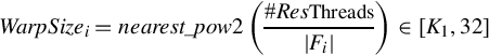
where #ResThreads refers to the maximum number of resident threads.
• Dynamic parallelism. In the case of vertices with degrees much greater than average (e.g., scale-free networks or graphs with power-law distribution in general), BFS-4K applies the dynamic parallelism provided by the Kepler architecture instead of virtual warps. Dynamic parallelism implies an overhead that, if not properly used, may worsen the algorithm performance. BFS-4K checks, at runtime, the characteristics of the frontier to decide whether and how to apply this technique.
• Edge-discover. With the edge-discover technique, threads are assigned to edges rather than vertices to improve thread workload balancing during frontier propagation. The edge-discover technique makes intense use of warp shuffle instructions. BFS-4K checks, at each propagation step, the frontier configuration to apply this technique rather than dynamic virtual warps. BFS-4K implements thread assignment through a binary search based on warp shuffle instructions. The algorithm performs the following steps:
1. Each warp thread reads a frontier vertex and saves the degree and the offset of the first edge.
2. Each warp computes the warp shuffle prefix-sum on the vertices’ degree.
3. Each thread of the warp performs a warp shuffle binary search of the own warp id (i.e., laneid ∈{0, …, 31}) on the prefix-sum results. The warp shuffle instructions guarantee the efficiency of the search steps (which are less than ![]() per warp).
per warp).
4. The threads of warp share, at the same time, the offset of the first edge with another warp shuffle operation.
5. Finally, the threads inspect the edges and store possible new vertices on the local queue.
• Single-block vs multiblock kernel. BFS-4K relies on a two-kernel implementation. The two kernels are used alternately and combined with the preceding features presented during frontier propagation.
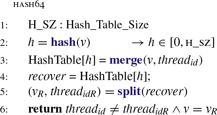
• A duplicate detection and correction strategy. This strategy is based on hash table and eight-bank access mode to sensibly reduce the memory accesses and improve the detection capability. BFS-4K implements a hash table in shared memory (i.e., one per streaming multiprocessor) to detect and correct duplicates and takes advantage of the eight-bank shared memory mode of Kepler to guarantee high performance of the table accesses. At each propagation step, each frontier thread invokes the hash64 procedure depicted in Algorithm 3 to update the hash table with the visited vertex (v). Given the size of the hash table (Hash_Table_Size), each thread of a block calculates the address (h) in the table for v (row 2). The thread identifier (threadid) and the visited vertex identifier (v) are merged into a single 64-bit word, to be saved in the calculated address (row 3). The merge operation (as well as the consequential split in row 5) is efficiently implemented through bitwise instructions. A duplicate vertex causes the update of the hash table in the same address by more threads. Thus each thread recovers the two values in the corresponding address (rows 4 and 5) and checks whether they have been updated (row 6) to notify a duplicate.
• Coalesced read/write memory accesses. To reduce the overhead caused by the many accesses in global memory, BFS-4K implements a technique to induce coalescence among warp threads through warp shuffle.
BFS-4K exploits the features of the Kepler architecture, such as dynamic parallelism, warp-shuffle, and eight-bank access mode, to guarantee an efficient implementation of the previously listed characteristics. Table 2 summarizes the differences between the most representative state-of-the-art BFS implementations and BFS-4K, while Fig. 5 reports a representative comparison of speedups among the BFS implementations for GPUs presented in Section 2.1, BFS-4K, and the sequential counterpart.
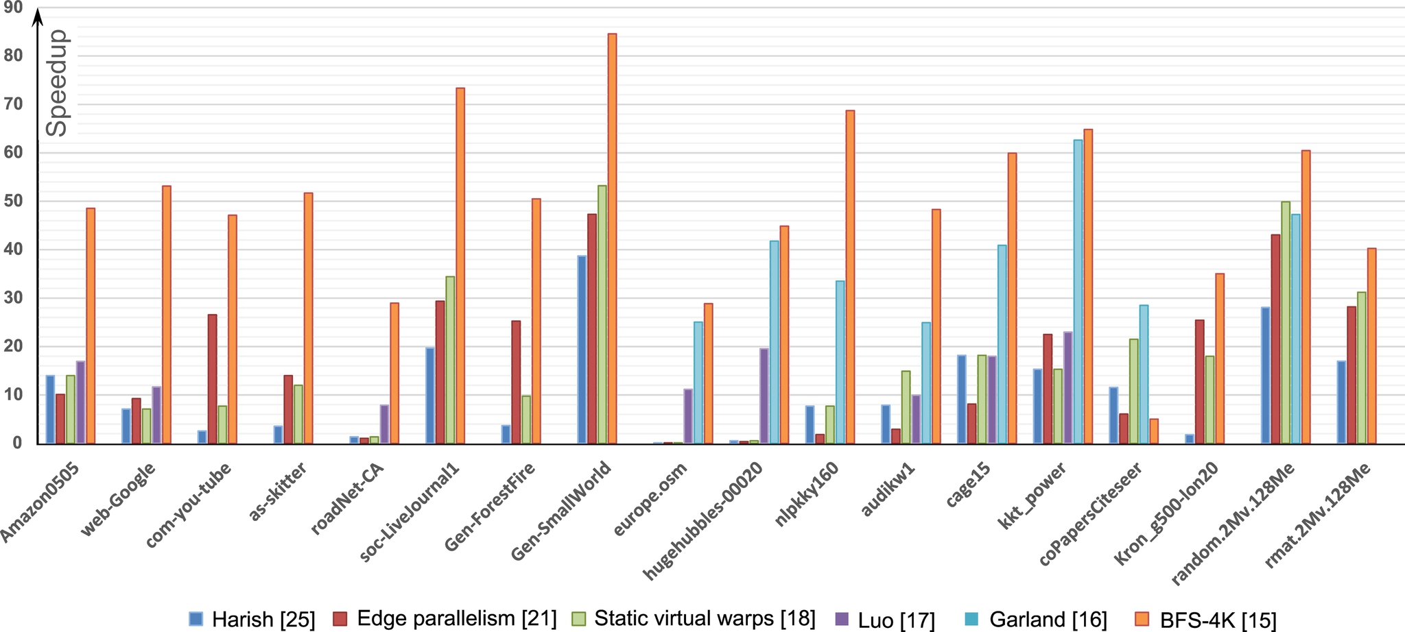
Table 2
Comparison of the Most Representative State-of-the-Art BFS Implementations With BFS-4K
| Harish [25] | Virtual Warps [18] | Edge Parallelism [21] | Luo [17] | Garland [16] | BFS-4K [15] | |
| Work complexity | O(V D + E) | O(V D+E) | O(ED) | O(V + E) | O(V + E) | O(V + E) |
| Space complexity | O(3V + E) | O(2V +E) | O(2E) | N/A | Ω(4V + 2E) | Ω(4V + E) |
| Type of parallelism | Vertices | Virtual warp | Edges | Vertices | Vertices, edges, CTA | Vertices, edges, dynamic virtual warp, dynamic parallelism |
| High-degree vertex management | No | Yes | Indifferent | No | Yes | Yes |
| Duplicate detection | No | No | No | No | Yes | Yes |
| Type of synchronization | Host-device | Host-device | Host-device | Host-device, interblock [27], thread barriers | Host-device, interblock [27] | Host-device, interblock [27], thread barriers |
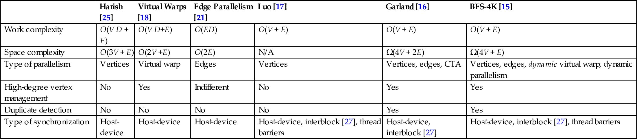
The results show how BFS-4K outperforms all the other implementations in every graph. This is due to the fact that BFS-4K exploits the more advanced architecture characteristics (in particular, Kepler features) and that it allows the user to optimize the visiting strategy through different knobs.
3 The single-source shortest path (SSSP) problem
Given a weighted graph G = (V, E), where V is the set of vertices and ![]() is the set of edges, the SSSP problem consists of finding the shortest paths from a single source vertex to all other vertices [1]. Such a well-known and long-studied problem arises in many different domains, such as road networks, routing protocols, artificial intelligence, social networks, data mining, and VLSI chip layout.
is the set of edges, the SSSP problem consists of finding the shortest paths from a single source vertex to all other vertices [1]. Such a well-known and long-studied problem arises in many different domains, such as road networks, routing protocols, artificial intelligence, social networks, data mining, and VLSI chip layout.
The de facto reference approaches to SSSP are the Dijkstra [34] and Bellman-Ford [35, 36] algorithms. The Dijkstra algorithm, by utilizing a priority queue where one vertex is processed at a time, is the most efficient, with a computational complexity almost linear to the number of vertices (![]() . Nevertheless, in several application domains where the modeled data maps to very large graphs involving millions of vertices, Dijkstra’s sequential implementation becomes impractical. In addition, since the algorithm requires many iterations and each iteration is based on the ordering of previously computed results, it is poorly suited for parallelization.
. Nevertheless, in several application domains where the modeled data maps to very large graphs involving millions of vertices, Dijkstra’s sequential implementation becomes impractical. In addition, since the algorithm requires many iterations and each iteration is based on the ordering of previously computed results, it is poorly suited for parallelization.
On the other hand, the Bellman-Ford algorithm relies on an iterative process over all edge connections, which updates the vertices continuously until final distances converge. Even though it is less efficient than Dijkstra’s (O(|V ||E|)), it is well suited to parallelization [37].
In the context of parallel implementations for GPUs, where the energy and power consumption is becoming a constraint in addition to performance [38], an ideal solution to SSSP would provide both the performance of the Bellman-Ford algorithm and the work efficiency of the Dijkstra algorithm. In the last years, some work was done to analyze the spectrum between massive parallelism and efficiency, and different parallel solutions for GPUs have been proposed to implement parallel-friendly and work-efficient methods to solve SSSP [39]. Experimental results confirmed that these trade-off methods provide a fair speedup by doing much less work than traditional Bellman-Ford methods while adding only a modest amount of extra work over serial methods.
On the other hand, none of these solutions, as well as Dijkstra’s implementations, work in graphs with negative weights [1]. The Bellman-Ford algorithm is the only solution that can also be applied in application domains where the modeled data maps on graphs with negative weights, such as power allocation in wireless sensor networks [40, 41], systems biology [42], and regenerative braking energy for railway vehicles [43].
3.1 The SSSP Implementations for GPUs
The Dijkstra and Bellman-Ford algorithms span a parallel versus efficiency spectrum. Dijkstra allows the most efficient (![]() ) sequential implementations [44, 45] but exposes no parallelism across vertices. Indeed, the solutions proposed to parallelize the Dijkstra algorithm for GPUs are shown to be asymptotically less efficient than the fastest CPU implementations [46, 47]. On the other hand, at the cost of lower efficiency (O(V E)), the Bellman-Ford algorithm is shown to be more easily parallelizable for GPUs by providing speedups of up to two orders of magnitude with respect to the sequential counterpart [14, 37].
) sequential implementations [44, 45] but exposes no parallelism across vertices. Indeed, the solutions proposed to parallelize the Dijkstra algorithm for GPUs are shown to be asymptotically less efficient than the fastest CPU implementations [46, 47]. On the other hand, at the cost of lower efficiency (O(V E)), the Bellman-Ford algorithm is shown to be more easily parallelizable for GPUs by providing speedups of up to two orders of magnitude with respect to the sequential counterpart [14, 37].
Meyer and Sanders [48] propose the Δ-stepping algorithm, a trade-off between the two extremes of Dijkstra and Bellman-Ford. The algorithm involves a tunable parameter Δ, whereby setting Δ = 1 yields a variant of the Dijsktra algorithm, while setting ![]() yields the Bellman-Ford algorithm. By varying Δ in the range
yields the Bellman-Ford algorithm. By varying Δ in the range ![]() , we get a spectrum of algorithms with varying degrees of processing time and parallelism.
, we get a spectrum of algorithms with varying degrees of processing time and parallelism.
Meyer and Sanders [48] show that a value of Δ = Θ(1/d), where d is the degree, gives a good tradeoff between work-efficiency and parallelism. In the context of GPU, Davidson et al. [39] selects a similar heuristic, Δ = cw/d, where d is the average degree in the graph, w is the average edge weight, and c is the warp width (32 on our GPUs).
Crobak et al. [49] and Chakaravarthy et al. [50] present two different solutions to efficiently expose parallelism of this algorithm on the massively multithreaded shared memory system IBM Blue Gene/Q.
Parallel SSSP algorithms for multicore CPUs were also proposed by Kelley and Schardl [51], who presented a parallel implementation of Gabow’s scaling algorithm [52] that outperforms Dijkstra’s on random graphs. Shun and Blelloch [53] presented a Bellman-Ford scalable parallel implementation for CPUs on a 40-core machine. Over the last ten years, several packages were developed for processing large graphs on parallel architectures, including the Parallel Boost Graph Library [54], Pregel [55], and Pegasus [56].
In the context of GPUs, Davidson et al. [39] propose three different work-efficient solutions for the SSSP problem. The first two, Near-Far Pile and Workfront Sweep, are the most representative state-of-the-art implementations. Workfront Sweep implements a queue-based Bellman-Ford algorithm that reduces redundant work because of duplicate vertices during the frontier propagation. Such a fast graph traversal method relies on the merge path algorithm [22], which equally assigns the outgoing edges of the frontier to the GPU threads at each algorithm iteration. Near-Far Pile refines the Workfront Sweep strategy by adopting two queues similarly to the Δ-Stepping algorithm. Davidson et al. [39] also propose the bucketing method to implement the Δ-Stepping algorithm. Δ-Stepping algorithm is not well suited for SIMD architectures as it requires dynamic data structures for buckets. However, the authors provide an algorithm implementation based on sorting that, at each step, emulates the bucket structure. The Bucketing and Near-Far Pile strategies greatly reduce the amount of redundant work with respect to the Workfront Sweep method, but at the same time, they introduce overhead for handling more complex data structure (i.e., frontier queue). These strategies are less efficient than the sequential implementation on graphs with large diameters because they suffer from thread underutilization caused by such unbalanced graphs.
3.2 H-BF: An Efficient Implementation of the Bellman-Ford Algorithm
Given a graph G(V, E), a source vertex s, and a weight function ![]() , the Bellman-Ford algorithm visits G and finds the shortest path to reach every vertex of V from source s. Algorithm 4 summarizes the original sequential algorithm, where the Relax procedure of an edge (u, v) with weight w verifies whether, starting from u, it is possible to improve the approximate (tentative) distance to v (which we call d(v)) found in any previous algorithm iteration. The relax procedure can be summarized as follows:
, the Bellman-Ford algorithm visits G and finds the shortest path to reach every vertex of V from source s. Algorithm 4 summarizes the original sequential algorithm, where the Relax procedure of an edge (u, v) with weight w verifies whether, starting from u, it is possible to improve the approximate (tentative) distance to v (which we call d(v)) found in any previous algorithm iteration. The relax procedure can be summarized as follows:
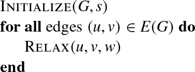
The algorithm, whose asymptotic time complexity is O(|V ||E|), updates the distance value of each vertex continuously until final distances converge.
H-BF [57] is a parallel implementation of the Bellman-Ford algorithm based on frontier propagation. Differently from all the approaches in literature, H-BF implements several techniques to improve the algorithm performance and, at the same time, to reduce the useless work done for solving SSSP involved by the parallelization process. H-BF implements such techniques by exploiting the features of the most recent GPU architectures, such as dynamic parallelism, warp-shuffle, read-only cache, and 64-bit atomic instructions.
The complexity of an SSSP algorithm is strictly related to the number of relax operations. The Bellman-Ford algorithm performs a higher number of relax operations than Dijkstra or Δ-Stepping algorithms, while on the other hand, it provides simple and lightweight management of the data structures. The relax operation is the most expensive in the Bellman-Ford algorithm, and in particular, in a parallel implementation, each relax involves an atomic instruction for handling race conditions, which takes much more time than a common memory access.
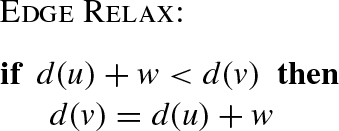
To optimize the number of relax operations, H-BF implements the graph visit by exploiting the concept of frontier. For this problem, the frontier, F, is an FIFO queue that, at each algorithm iteration, contains active vertices—that is, all and only vertices whose tentative distance has been modified and which therefore must be considered for the relax procedure at the next iteration. Given a graph G and a source vertex s, the parallel frontier-based algorithm can be summarized in Algorithm 5, where adj[u] returns the neighbors of vertex u. Fig. 6 shows an example of the basic algorithm iterations starting from vertex “0,” where F is the active vertex queue and D is the corresponding data structure containing the tentative distances. The example shows, for each algorithm iteration, the dequeue of each vertex form the frontier, the corresponding relax operations, that is, the distance updating for each vertex (if necessary), and the vertex enqueues in the new frontier. In the example, the algorithm converges in a total of five relax operations over five iterations.

The frontier structure is similar to that applied for implementing the parallel BFS presented in Section 2.1. The main difference from BFS is the number of times a vertex can be inserted in the queue. In BFS, a vertex can be inserted in such a queue only once, while, in the Bellman-Ford implementation, a vertex can be inserted O(|E|) times in the worst case.
Fig. 7 summarizes the speedup of the different implementations with respect to the sequential frontier-based Bellman-Ford implementation. The results show how H-BF outperforms all the other implementations in every graph. The speedup on graphs with very high diameter (leftmost side of the figure) is quite low for every parallel implementation. This is due to the very low degree of parallelism for propagating the frontier in such graph typology. In these graphs, H-BF is the only parallel implementation that outperforms the Boost Dijkstra solution in asia.osm, and it preserves comparable performance in USA-road.d-CAL. On the other hand, in the literature, the sequential Boost Dijkstra implementation largely outperforms all the other parallel solutions.
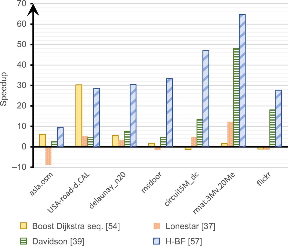
H-BF provides the best performance (time and MTEPS) on the graphs on the rightmost side of Fig. 7. H-BF also provides high speedup in rmat.3Mv.20Me and flickr, which are largely unbalanced graphs. This underlines the effectiveness of H-BF to deal with such an unbalancing problem in traversing graphs. The optimization based on the 64-bit atomic instruction strongly impacts the performance of graphs with small diameters. This is due to the fact that such graph visits are characterized by a rapid grow of the frontier, which implies a high number of duplicate vertices. The edge classification technique implemented in H-BF successfully applies to the majority of the graphs. In particular, asia.osm has a high number of vertices with an in-degree equal to one, while in msdoor and circuit5M_dc each vertex has a self-loop. Scale-free graphs (e.g., rmat.3Mv.20Me and flickr) are generally characterized by a high number of vertices with a low out-degree.
4 The APSP problem
APSP is a fundamental problem in computer science that finds application in different fields such as transportation, robotics, network routing, and VLSI design. The problem is to find paths of minimum weight between all pairs of vertices in graphs with weighted edges. The common approaches to solving the APSP problem rely on iterating the SSSP algorithm from all vertices (Johnson algorithm), matrix multiplication, and the Floyd-Warshall algorithm.
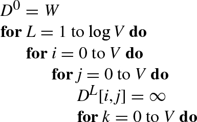
The Johnson algorithm performs the APSP in two steps. First, it detects the negative cycles by applying the Bellman-Ford algorithm and then it runs the Dijsktra algorithm from all vertices. This approach has ![]() time complexity and is suitable only for sparse graphs. The second approach applies the matrix multiplication over min, plus semiring to compute the APSP in
time complexity and is suitable only for sparse graphs. The second approach applies the matrix multiplication over min, plus semiring to compute the APSP in ![]() . The matrix multiplication method derives from the following recursive procedure. Letting wij be the weight of edge (i, j), wii = 0 and dijℓ be the shortest path from i to j using ℓ or fewer edges, we compute dijℓ by using the recursive definition:
. The matrix multiplication method derives from the following recursive procedure. Letting wij be the weight of edge (i, j), wii = 0 and dijℓ be the shortest path from i to j using ℓ or fewer edges, we compute dijℓ by using the recursive definition:
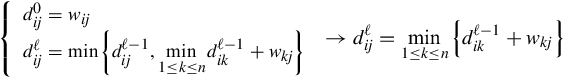
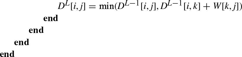
We note that making the substitutions ![]() and + →⋅, the definition is equivalent to the matrix multiplication procedure. Algorithm 6 reports the pseudocode.
and + →⋅, the definition is equivalent to the matrix multiplication procedure. Algorithm 6 reports the pseudocode.
Finally, the Floyd-Warshall algorithm, which is the standard approach for the APSP problem in the case of edges with negative weights, does not suffer from performance degradation for dense graphs. The algorithm has O(|V |3) time complexity and requires O(|V |2) memory space.
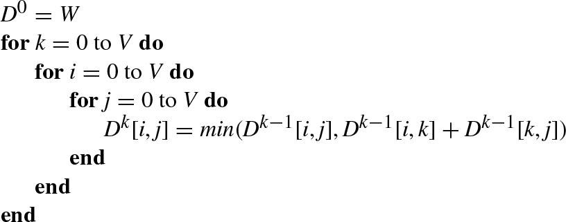
With G = (V, E) being a weighted graph with an edge-weight function ![]() and W = w(i, j) representing the weighted matrix, we have the pseudocode of the algorithm as shown in Algorithm 7.
and W = w(i, j) representing the weighted matrix, we have the pseudocode of the algorithm as shown in Algorithm 7.
4.1 The APSP Implementations for GPUs
The first GPU solution for the APSP problem was proposed by Harish and Narayanan [25], who used their parallel SSSP algorithm from all vertices of the graph. Also Ortega et al. [58] resolved the APSP problem in the same way, by proposing a highly tunable GPU implementation of the Dijkstra algorithm.
The most important idea, which provided the basis for a subsequent efficient GPU implementations of the Floyd-Warshall algorithm was proposed by Venkataraman et al. [3] in the context of multicore CPUs. The proposed solution takes advantage of the cache utilization. It first partitions the graph matrix into multiple tiles that fit in cache, and then it iterates on each tile multiple times. In particular, such a blocked Floyd-Warshall algorithm comprises three main phases (Fig. 8).
1. The computation in each iteration starts from a tile in the diagonal of the matrix, from the upper-left to the lower-right. Each tile in the diagonal is independent of the rest of the matrix and can be processed in place.
2. In the second phase, all tiles that are in the same row and in the same column of the independent tiles are computed in parallel. All tiles in this phase are dependent only on itself and on the independent tiles.
3. In the third phase, all remaining tiles are dependent from itself and from the main row and the main column that were computed in the previous phase.
The blocked Floyd-Warshall algorithm was implemented for GPU architectures by Katz and Kider [4], who strongly exploited the shared memory as local cache. Lund et al. [5] improved such a GPU implementation by optimizing the use of registers and by taking advantage of memory coalescing. Buluç et al. [6] presented a recursive formulation of the APSP based on the Gaussian elimination (LU) and matrix multiplication with O(|V |3) complexity, which exposes a good memory locality.
Later, Harish et al. [59] revisited the APSP algorithm based on matrix multiplication, and they presented two improvements: streaming blocks and lazy minimum evaluation. The streaming block optimization describes a method to partition the adjacency matrix and to efficiently transfer each partition to the device through asynchronous read and write operations. The second optimization aims at decreasing the arithmetic computation by avoiding the minimum operation when one operand is set to infinite. The presented algorithm achieves a speedup from 5 to 10 over Katz and Kider algorithm. Nevertheless, it is slower than the Gaussian elimination method of Buluç et al. On the other hand, they showed that their algorithm is more scalable and that the optimization of the lazy minimum evaluation is not orthogonal to the Gaussian elimination method.
Tran et al. [9] proposed an alternative algorithm based on matrix multiplication and on the repeated squaring technique (Algorithm 6). It outperforms the base Floyd-Warshall algorithm when the graph matrix exceeds the GPU memory.
Matsumoto et al. [7] proposed a hybrid CPU-GPU based on OpenCL, which combines the blocked Floyd-Warshall algorithm for a coarse-grained partition of the graph matrix and the matrix multiplication as a main procedure.
Finally, Djidjev et al. [8] proposed an efficient implementation of APSP on multiple GPUs for graphs that have good separators.
5 Load Balancing and Memory Accesses: Issues and Management Techniques
Load unbalancing and noncoalesced memory accesses are the main problems when implementing any graph algorithm for GPUs. The two are caused by the nonhomogeneity of real graphs. Different techniques have been presented in the literatures to decompose and map the graph algorithm workload to threads [15, 16, 18, 25,60–62]. All these techniques differ in terms of the complexity and in terms of the overhead they introduce in an application’s execution. The simplest solutions [18, 25] apply best to very regular workloads, but they cause strong unbalancing and consequently loss of performance in irregular workloads. More complex solutions [15, 16,60–62] apply best to irregular problems through semidynamic or dynamic workload-to-thread mappings. Nevertheless, the overhead introduced for such a mapping often worsens the overall performance of an application when run on regular problems.
In general, the techniques for decomposing and mapping a workload to GPU threads for graph applications rely on the prefix-sum data structure2 [16]. Given a workload to be allocated (e.g., a set of graph vertices or edges) over GPU threads, prefix-sum calculates the offsets to be used by the threads to access the corresponding work-units (fine-grained mapping) or to block work-units, which we call work-items (coarse-grained mapping). All these decomposition and mapping techniques can be organized in three classes: Static mapping, semidynamic mapping, and dynamic mapping.
5.1 Static Mapping Techniques
This class includes all the techniques that statistically assign each work-item (or blocks of work-units) to a corresponding GPU thread. This strategy allows to considerably reduce the overhead for calculating the work-item to thread mapping during the application execution, but on the other hand, it suffers from load unbalancing when the work-units are not regularly distributed over the work-items. The most important techniques are summarized in the following sections.
5.1.1 Work-items to threads
This approach represents the simplest and fastest mapping method by which each work-item is mapped to a single thread [25]. Fig. 9A shows an example in which eight items are assigned to a corresponding number of threads. For the sake of clarity, only four threads per warp are considered in the example, which underlines two levels of possible unbalancing of this technique. First, irregular (i.e., unbalanced) work-items mapped to threads of the same warp cause the warp threads to be in idle state (i.e., branch divergence). t1, t3, and t0 of warp0 in Fig. 9A are examples. Then irregular work-items cause whole warps to be in idle state (e.g., warp0 w.r.t. warp1 in Fig. 9A). In a third level of unbalancing, this technique can cause whole blocks of threads to be in idle state.
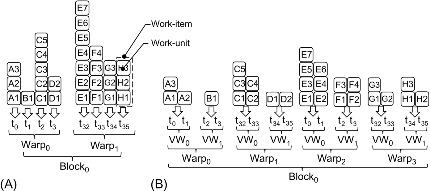
In addition, considering that work-units of different items are generally stored in nonadjacent addresses in global memory, this mapping strategy leads to sparse and noncoalesced memory accesses. As an example, threads t0, t1, t2, and t3 of Warp0 concurrently access to the nonadjacent units A1, B1, C1, and D1, respectively. For all these reasons, this technique is suitable for applications running on very regular data structures, in which any more-advanced mapping strategies will run at runtime (as explained in the following paragraphs), leading to unjustified overhead.
5.1.2 Virtual warps
This technique consists of assigning chunks of work-units to groups of threads called virtual warps, where the virtual warps are equally sized and the threads of a virtual warp belong to the same warp [18]. Fig. 9B shows an example in which the chunks correspond to the work-items and, for the sake of clarity, the virtual warps have a size equal to two threads. Virtual warps allow the workload assigned to threads of the same group to be almost equal, and consequently it allows reducing branch divergence. In addition, this technique improves the coalescing of memory accesses since more threads of a virtual warp have access to adjacent addresses in global memory (e.g., t0, t1 of Warp2 in Fig. 9B). These improvements are proportional to the virtual warp size. Increasing the warp size leads to reducing branch divergence and better coalescing the work-unit accesses in global memory. Nevertheless, virtual warps have several limitations. First, the maximum size of virtual warps is limited by the number of available threads in the device. Given the number of work-items and a virtual warp size, the required number of threads is expressed as follows:
If such a number is greater than the available threads, the work-item processing is serialized with a consequent decrease of performance. Indeed, a wrong sizing of the virtual warps can impact the application performance. In addition, this technique provides good balancing among threads of the same warp, while it does not guarantee good balancing among different warps or among different blocks. Finally, another major limitation of such a static mapping approach is that the virtual warp size has to be fixed statically. This represents a major limitation when the number and size of the work-items change at runtime.
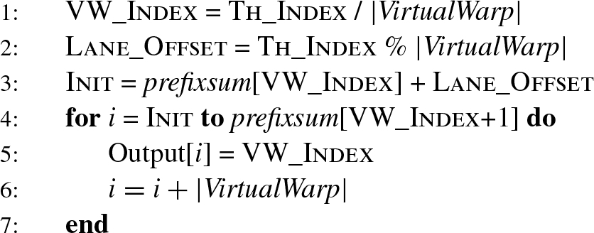
The algorithm run by each thread to access the corresponding work-units is summarized as in Algorithm 8, where VW_Index and LANE_Offset are the virtual warp index and offset for the thread (e.g., V W0, and 0 for t0 in Fig. 9B), Init represents the starting work-unit id, and the for cycle represents the accesses of the thread to the assigned work-units (e.g., A1, A3 for t0 and A2 for t1).
5.2 Semidynamic Mapping Techniques
This class includes the techniques by which different mapping configurations are calculated statically, and at runtime, the application switches among them.
5.2.1 Dynamic virtual warps + dynamic parallelism
This technique was introduced in Ref. [15] and relies on two main strategies. First, it implements a virtual warp strategy in which the virtual warp size is calculated and set at runtime depending on the workload and work-item characteristics (i.e., size and number). At each iteration, the right size is chosen among a set of possible values, which spans from 1 to the maximum warp size (i.e., 32 threads for NVIDIA GPUs, 64 for AMD GPUs). For performance reasons, the range is reduced to a power of two values only. Considering that a virtual warp size equal to one has the drawbacks of the work-item to thread technique and that memory coalescence increases proportionally with the virtual warp size (see Section 5.1.2), sizes that are too small are excluded from the range a priori. The dynamic virtual warp strategy provides a fair balancing in irregular workloads. Nevertheless, it is inefficient in cases of few and very large work-items (e.g., in datasets representing scale-free networks or graphs with power-law distribution in general).
On the other hand, dynamic parallelism, which exploits the most advanced features of the GPU architectures (e.g., from NVIDIA Kepler on) [30], allows recursion to be implemented in the kernels and thus threads and thread blocks to be dynamically created and properly configured at runtime without requiring kernel returns. This approach allows fully addressing the work-item irregularity. Nevertheless, the overhead introduced by the dynamic kernel stack may override this feature’s advantages if it is replicated unconditionally for all the work-items [15].
To overcome these limitations, dynamic virtual warps and dynamic parallelism are combined into a single mapping strategy and applied alternatively at runtime. The strategy applies dynamic parallelism to the work-items having size greater than a threshold, and it applies dynamic virtual warps to the others. It applies best to applications with few and strongly unbalanced work-items that may vary at runtime (e.g., applications for sparse graph traversal). This technique guarantees load balancing among threads of the same warps and among warps. It does not guarantee balancing among blocks.
5.2.2 CTA + warp + scan
In the context of graph traversal, Merrill et al. [16] proposed an alternative approach to the load balancing problem. Their algorithm consists of three steps:
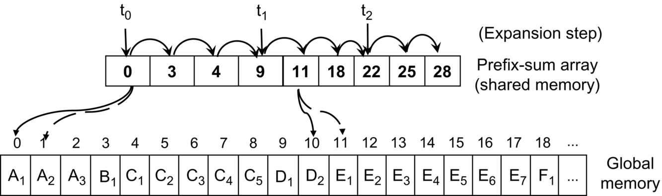
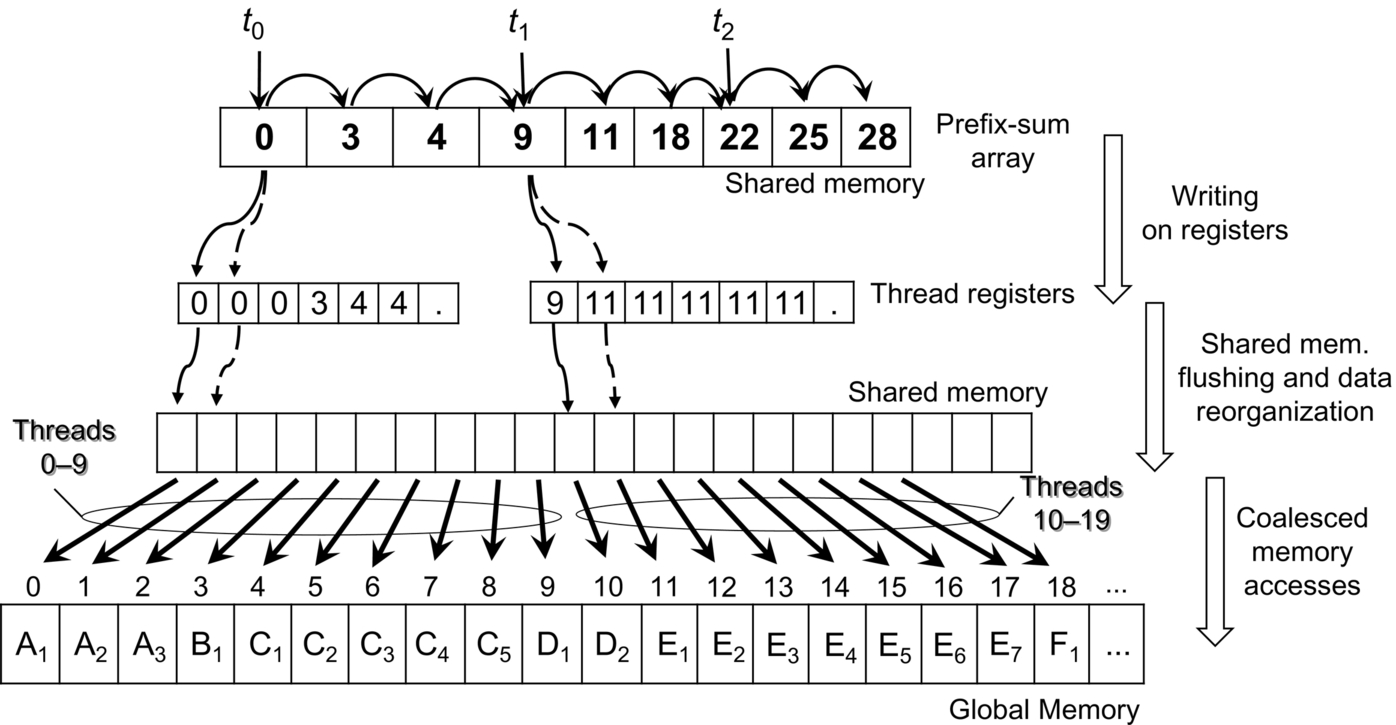
1. All threads of a block access the corresponding work-item (through the work-item to thread strategy) and calculate the item sizes. The work-items with sizes greater than a threshold (CTATH) are nondeterministically ordered, and are one at a time (i) copied in the shared memory, and (ii) processed by all the threads of the block (called cooperative thread array [CTA]). The algorithm (see Algorithm 9) for such a first step, which is called strip-mined gathering) is run by each thread (ThID).
In the pseudocode, row 3 implements the nondeterministic ordering (based on iterative match/winning among threads), rows 5–8 calculate information on the work-item to be copied in shared memory, while rows 10–14 implement the item partitioning for the CTA. This phase introduces sensible overhead for the two CTA synchronizations, and rows 5–8 are run by one thread only.
2. In the second step, the strip-mined gathering is run with a lower threshold (WarpTH) and at warp level. That is, it targets smaller work-items, and a cooperative thread array consists of threads of the same warp. This allows avoiding any synchronization among threads (as they are implicitly synchronized in SIMD—like fashion in the warp) and addressing work-items with sizes proportional to the warp size.
3. In the third step, the remaining work-items are processed by all block threads. The algorithm computes a block-wide prefix-sum on the work-items and stores the resulting prefix-sum array in the shared memory. Finally, all threads of the block have use of such an array in order to access the corresponding work-unit. If the array size exceeds the shared memory space, the algorithm iterates.
This strategy provides a perfect balancing among threads and warps. On the other hand, the strip-mined gathering procedure run at each iteration introduces a enough overhead to slow down an application’s performance in the case of quite regular workloads. The strategy works well only in cases of very irregular workloads.
5.3 Dynamic Mapping Techniques
Contrary to static mapping, the dynamic mapping approaches achieve perfect workload partition and balancing among threads at the cost of additional computation at runtime. The core of such a computation is the binary search over the prefix-sum array. The binary search aims at mapping work-units to the corresponding threads.
5.3.1 Direct search
Given the exclusive prefix-sum array of the work-unit addresses stored in global memory, each thread performs a binary search over the array to find the corresponding work-item index. This technique provides perfect balancing among threads (i.e., one work-unit is mapped to one thread), warps, and blocks of threads. Nevertheless, the large size of the prefix-sum array involves an arithmetic-intensive computation (i.e., #threads × binarysearch()) and all the accesses performed by the threads to solve the mapping very scattered. This often eludes the benefit of the provided perfect balancing.
5.3.2 Local warp search
To reduce both the binary search computation and the scattered accesses to the global memory, this technique first loads chunks of the prefix-sum array from the global memory to the shared memory. Each chunk consists of 32 elements, which are loaded by 32 warp threads through a coalesced memory access. Then each thread of the warp performs a lightweight binary search (i.e., maximum ![]() steps) over the corresponding chunk in the shared memory.
steps) over the corresponding chunk in the shared memory.
In the context of graph traversal, this approach was further improved by exploiting data locality in registers [15]. Instead of working on shared memory, each warp thread stores the workload offsets in their own registers and then performs a binary search by using Kepler warp-shuffle instructions [30].
In general, the local warp search strategy provides a very fast work-units to threads mapping and guarantees coalesced accesses to both the prefix-sum array and the work-units in global memory. On the other hand, since the sum of work units included in each chunk of the prefix-sum array is greater than the warp size, the binary search on the shared memory (or registers for the enhanced version for Kepler) is repeated until all work-units are processed. This leads to more work-units being mapped to the same thread. Indeed, although this technique guarantees a fair balancing among threads of the same warp, it suffers from a work unbalance between different warps since the sum of work-units for each warp cannot be uniform in general. For the same reason, it does not guarantee balancing among blocks of threads.
5.3.3 Block search
To deal with the local warp search limitations, Davidson et al. [60] introduced the block search strategy through cooperative blocks. Instead of warps performing 32-element loads, in this strategy each block of threads loads a maxi chunk of prefix-sum elements from the global to the shared memory, where the maxi chunk is as large as the available space in shared memory for the block. The maxi chunk size is equal for all the blocks. Each maxi chunk is then partitioned by considering the amount of work-units included and the number of threads per block. Finally, each block thread performs only one binary search to find the corresponding slot. With the block search strategy, all the units included in a slot are mapped to the same thread. This leads to several advantages. First, all the threads of a block are perfectly balanced. The binary searches are performed in shared memory, and the overall amount of searches is sensibly reduced (i.e., they are equal to the block size). Nevertheless, this strategy does not guarantee balancing among different blocks. This is due to the fact that the maxi chunk size is equal for all the blocks, but the chunks can include a different amount of work-units. In addition, this strategy does not guarantee memory coalescing among threads when they access the assigned work-units. Finally, this strategy cannot exploit advanced features for intrawarp communication and synchronization among threads, for example, warp shuffle instructions.
5.3.4 Two-phase search
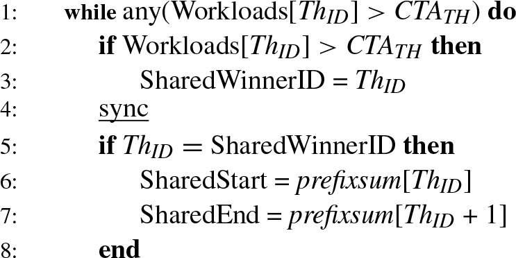
Davidson et al. [60], Green et al. [61], and Baxter [62] proposed three equivalent methods to deal with the interblock load unbalancing. All the methods rely on two phases: partitioning and expansion.
First, the whole prefix-sum array is partitioned into balanced chunks, that is, chunks that point to the same amount of work-units. Such an amount is fixed as the biggest multiple of the block size that fits in the shared memory. As an example, in blocks of 128 threads with 2 prefix-sum chunks pointing to 128 × K units and 1300 slots in shared memory, K is set to 10. The chunk size may differ among blocks. The partition array, which aims at mapping all the threads of a block into the same chunk, is built as follows. One thread per block runs a binary search on the whole prefix-sum array in global memory by using its own global id times the block size (![]() . This allows for finding the chunk boundaries. The number of binary searches in global memory for this phase is equal to the number of blocks. The new partition array, which contains all the chunk boundaries, is stored in global memory.
. This allows for finding the chunk boundaries. The number of binary searches in global memory for this phase is equal to the number of blocks. The new partition array, which contains all the chunk boundaries, is stored in global memory.
In the expansion phase, all the threads of each block load the corresponding chunks into the shared memory (similarly to the dynamic techniques presented in the previous paragraphs). Then each thread of each block runs a binary search in such a local partition to get the (first) assigned work-unit. Each thread sequentially accesses all the assigned work units in global memory. The number of binary searches for the second step is equal to the block size. Fig. 10 shows an example of an expansion phase, in which three threads (t0, t1, and t2) of the same warp access the local chunk of a prefix-sum array to get the corresponding starting point of the assigned work-unit. Then they sequentially access the corresponding K assigned units (A1 − D1 for t0, D2 − F2 for t1, etc.) in global memory.
In conclusion, the two-phase search strategy allows the workload among threads, warps, and blocks to be perfectly balanced at the cost of two series of binary searches. The first is run in global memory for the partitioning phase, while the second, which most affects the overall performance, is run in shared memory for the expansion phase.
The number of binary searches for partitioning is proportional to the K parameter. High values of K involve fewer and bigger chunks to be partitioned and consequently fewer steps for each binary search. Nevertheless, the main problem of such a dynamic mapping technique is that the partitioning phase leads to very scattered memory accesses of the threads to the corresponding work-units (see bottom of Fig. 10). Such a problem worsens by increasing the K value.
5.4 The Multiphase Search Technique
As an improvement of the dynamic load balancing techniques just presented, Ref. [65] proposes the multiphase mapping strategy, which aims at exploiting the balancing advantages of the two-phase algorithms while overcoming the limitations concerning the scattered memory accesses. This technique consists of two main contributions: coalesced expansion and iterated search.
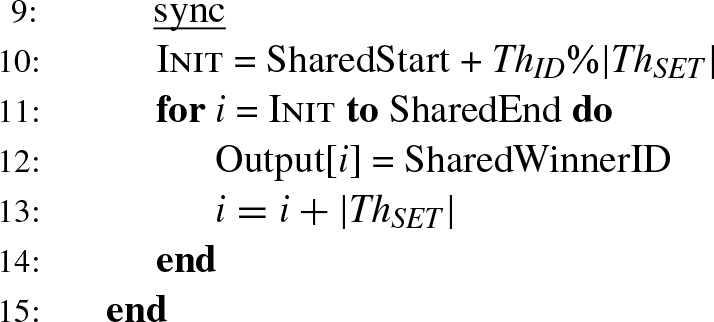
5.5 Coalesced Expansion
The expansion phase consists of three subphases, by which the scattered accesses of threads to the global memory are reorganized into coalesced transactions. This is done in shared memory and by taking advantage of local registers. The technique works for both reading and writing accesses to the global memory as does the two-phase approach. For the sake of clarity, we consider writing accesses in the following steps:
1. Instead of sequentially writing on the work-units in global memory, each thread sequentially writes a small amount of work-units in the local registers. Fig. 11 shows an example. The amount of units is limited by the available number of free registers.
2. After a thread block synchronization, the local shared memory is flushed, and the threads move and reorder the work-unit array from the registers to the shared memory.
3. Finally, the entire warp of threads cooperates for a coalesced transaction of the reordered data into the global memory. It is important to note that this step does not require any synchronization because each warp executes independently on its own slot of shared memory.
Steps 2 and 3 are iterated until all the work-units assigned to the threads are processed. Even though these steps involve some extra computations with respect to the direct writings, the achieved coalesced accesses in global memory significantly improve the overall performance.
5.6 Iterated Searches
The shared memory size and the size of thread blocks play an important role in the coalesced expansion phase. The bigger the block size, the shorter the partition array stored in shared memory. On the other hand, the bigger the block size, the greater the synchronization overhead among the block warps, and the more the binary search steps performed by each thread (see final considerations of the two-phase search in Section 5.3.4).
In particular, the overhead introduced to synchronize the threads after the writing on registers (see Step 1 of coalesced expansion) is the bottleneck of the expansion phase (each register writing step requires two barriers of thread). The iterated search optimization aims at reducing such an overhead as follows:
1. In the partition phase, the prefix-sum array is partitioned into balanced chunks. Differently from the two-phase search strategy, the size of such chunks is fixed as a multiple of the available space in shared memory as
where Blocksize × K represents the biggest number of work-units (i.e., a multiple of the block size) that fit in shared memory (as in the two-phase algorithm), while IS represents the iteration factor. The number of threads required in this step decreases linearly with IS.
2. Each block of threads loads from global to shared memory a chunk of the prefix-sum, performs the function initialization, and synchronizes all threads.
3. Each thread of a block performs IS binary searches on such an extended chunk.
4. Each thread starts with the first step of the coalesced expansion, that is, it sequentially writes an amount of work-units in the local registers. Such an amount is equal to IS times larger than in the standard two-phase strategy.
5. The local shared memory is flushed, and each thread moves a portion of the extended work-unit array from the registers to the shared memory. The portion size is equal to Blocksize × K. Then the entire warp of threads cooperates for a coalesced transaction of the reordered data into the global memory, as in the coalesced expansion phase. This step iterates IS times, until all the data stored in the registers have been processed.
With respect to the standard partitioning and expansion strategy, the iterated search optimization reduces the number of synchronization points by a factor of 2 * IS, avoids many block initializations, decreases the number of required threads, and maximizes the shared memory utilization during the loading of the prefix-sum values with many large consecutive intervals. Nevertheless, the required number of registers grows proportionally to the IS parameter. Considering that the maximum number of registers per thread is a fixed constraint for any GPU device (e.g., 32 for NVIDIA Kepler devices) and that exceeding such a constraint causes data to be spilled in L1 cache and then in L2 cache or global memory, values of IS that are too high may compromise the overall performance of the proposed approach.
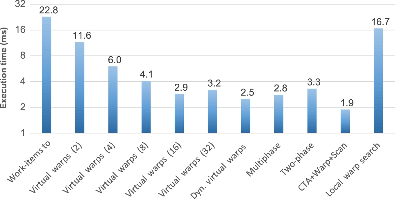
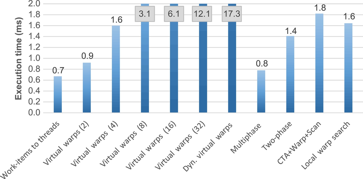
Figs. 12–15 summarize and compare the performance of each technique over different graphs, each one having very different characteristics and structures. The results obtained with the direct search and block search techniques are much worse than the other techniques and, for the sake of clarity, are not reported in the figures.
In the first benchmark (Fig. 12), as expected, work-items to threads is the most efficient balancing technique. This is due to the very regular workload and the small average work-item size. In this benchmark, any overhead for the dynamic item-to-thread mapping may compromise the overall algorithm performance. However, multiphase search is the second most efficient technique. This underlines the reduced overhead introduced by such a dynamic technique, which also applies well in cases of very regular workloads.
In the web-NotreDame benchmark (Fig. 13), multiphase search is the most efficient technique and provides almost twice the performance with respect to the second best techniques (virtual warps and two-phase). On the other hand, virtual warps provides good performance if the virtual warp size is properly set, while it may worsen with sizes that are set wrong. The virtual warp size must be set statically. For the obtained results in these two benchmarks, we noticed that the optimal virtual warp size is proportional and follows approximately the average for work-item sizes.

In these first two benchmarks, CTA + Warp + Scan, which is one of the most advanced, sophisticated, state-of-the-art balancing techniques, provides low performance. This is due to the fact that the CTA and the warp phases are never or rarely ever activated, while the activation controls involve heavy overhead.
Multiphase search also provides the best results in the circuit5M benchmark (Fig. 14). In such a benchmark, the CTA + Warp + Scan, two-phase search, and multiphase search dynamic techniques are one order of magnitude faster than the static-mapping techniques. In web-Notredame and in circuit5M, multiphase search shows the best results because of the low average (less than warp size) and high standard deviation.
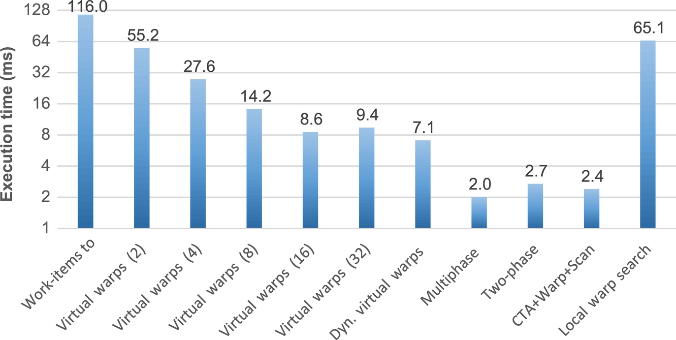
In the last benchmark, kron_g500-logn20 (Fig. 15), CTA + Warp + Scan provides the best results because the CTA and warp phases are frequently activated and exploited. However, the performance of multiphase is comparable. Dynamic virtual warps and virtual warps provide a similar performance. Indeed, these two techniques are very efficient on high-average datasets because, with a thread group size of 32, they completely avoid the warp divergence. Finally, the dynamic parallelism feature provided by Kepler, implemented in the corresponding semidynamic technique, is the best application only when the work-item sizes and their average are very large. In any case, in all the analyzed data sets, all the dynamic load balancing techniques, and in particular the multiphase search, performed better without such a feature.