
Accurately modeling GPGPU frequency scaling with the CRISP performance model
R. Nath; D. Tullsen University of California, San Diego, La Jolla, CA, United States
Abstract
CRItical Stalled Path (CRISP) is the first runtime analytical model of general-purpose computation on graphics processing unit (GPGPU) performance that models the effect of changing frequency. Prior models not targeted at a GPGPU fail to account for important characteristics of GPGPU execution, including the high degree of overlap between memory access and computation and the frequency of store-related stalls. CRISP provides significantly improved accuracy, being within 4% on average when scaling frequency by up to 7×. Using CRISP to drive a runtime energy efficiency controller yields a 10.7% improvement in energy-delay product versus 6.2% attainable via the best prior method.
Keywords
GPGPU; DVFS; Analytical model; Performance modeling
Acknowledgments
This work was supported in part by NSF grants CCF-1219059 and CCF-1302682.
1 Introduction
Dynamic voltage and frequency scaling (DVFS) [1] is employed in modern architectures to allow the system to adjust the frequency and supply voltage to particular components within the computer. DVFS has shown the potential for significant power and energy savings in many system components, including processor cores [2, 3], memory system [4–6], last level cache [7], and interconnect [8–10]. DVFS scales voltage and frequency for energy and power savings, but can also address other problems such as temperature [11], reliability [12], and variability [13]. However, in all cases it trades off performance for other gains, so properly setting DVFS to maximize particular goals can only be done with the assistance of an accurate estimate of the performance of the system at alternate frequency settings. In addition, we must be able to predict performance in a way that both tracks the dynamic behavior of the application over time and minimizes the measurement and computation overhead of the predictive model.
This chapter describes the CRItical Stalled Path (CRISP) performance predictor for general-purpose computation on graphics processing units (GPGPUs) under varying core frequency. Existing analytical models that account for frequency change target only CPU performance, and do not effectively capture the execution characteristics of a GPU.
While extensive research has been done on DVFS performance modeling for CPU cores, there is little guidance in the literature for GPU and GPGPU settings, despite the fact that modern GPUs have extensive support for DVFS [14–17]. In fact, the potential for DVFS on GPUs is high for at least two reasons. First, the maximum power consumption in a GPGPU is often higher than CPUs, for example, 250 W for the NVIDIA GTX480. Second, while the range of DVFS settings in modern CPUs is shrinking, that is not yet the case for GPUs, which have ranges such as 0.5–1.0 V (NVIDIA Fermi [18]).
This work presents a performance model that closely tracks GPGPU performance on a wide variety of workloads and that significantly outperforms existing models that are tuned to the CPU. The improvement is a result of key differences between CPU execution and GPU execution that are not handled by those models. We describe those differences and show how CRISP correctly accounts for them in its runtime model.
Existing CPU DVFS performance models fall into one of a few categories. Most are empirical and use statistical [19–23] or machine learning methods [24, 25], or assume a simple linear relationship [26–32] between performance and frequency. Abe et al. [14] target GPUs, but with a regression-based offline statistical model that is neither targeted for nor conducive to runtime analysis.
Recent research presents new performance counter architectures [33–35] to model the impact of frequency scaling on CPU workloads. These analytical models (eg, leading load [33] and critical path [34]) divide a CPU program into two disjoint segments representing the nonpipelined (TMemory) and pipelined (TCompute) portion of the computation. They make two assumptions: (a) the memory portion of the computation never scales with frequency and (b) cores never stall for store operations. Though these assumptions are reasonably valid in CPUs, they start to fail as we move to massively parallel architecture like GPGPUs. No existing runtime analytical models for GPGPUs handle the effect of voltage-frequency changes.
A program running on a GPGPU, typically referred to as a kernel, will have a high degree of thread-level parallelism. The single instruction multiple thread (SIMT) parallelism in GPGPUs allows a significant portion of the computation to be overlapped with memory latency, which can make the memory portion of the computation elastic to core clock frequency and thus breaks the first assumption of the prior models.
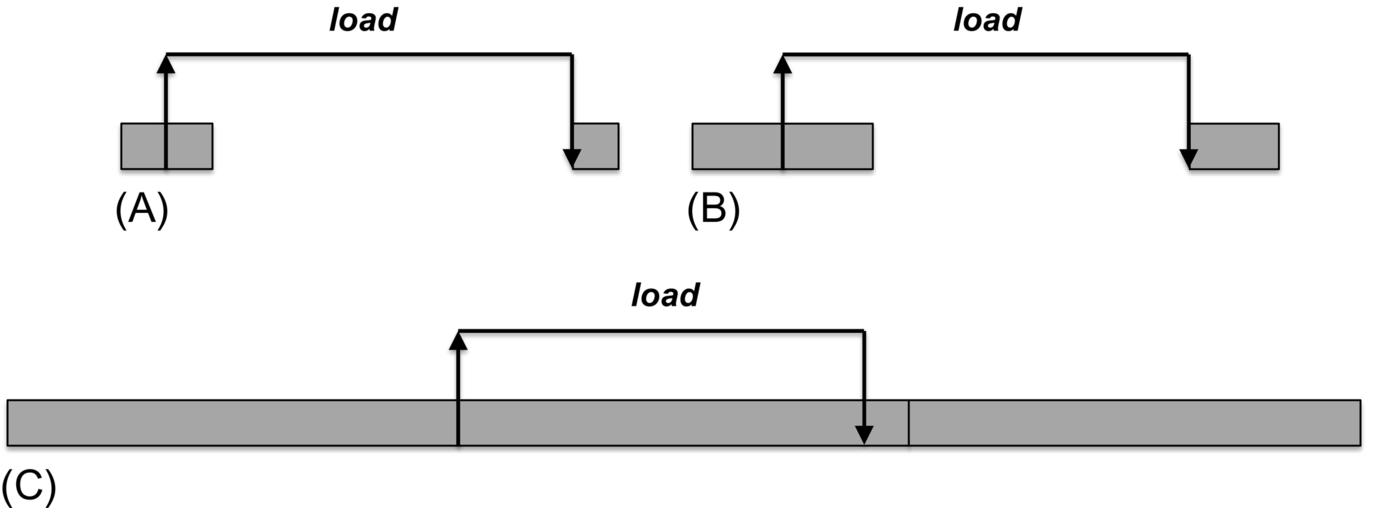
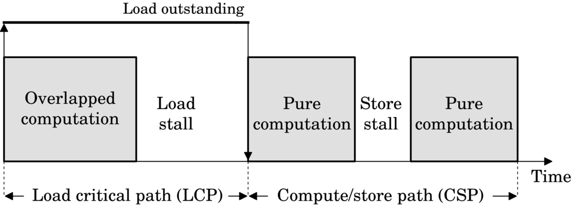
Figs. 1 and 2 show this phenomenon on CPU and GPGPU kernels at different core clock frequencies. A CPU program will typically have little memory-overlapped computation, because it runs one or few threads, and has limited storage for unretired instructions. Thus, in this illustrative example, the memory-bound region remains memory bound unless the clock frequency is scaled by extreme amounts. On a GPGPU, however, due to very high amounts of thread and SIMT parallelism, the memory-overlapped computation can be quite significant, and thus a small reduction in frequency may convert the region, or even the entire kernel, from memory bound to compute bound.
Though memory/computation overlap has been used for program optimization, modeling frequency scaling in the presence of abundant parallelism and high memory/computation overlap is a new, complex problem. Moreover, due to the wide single instruction multiple data (SIMD) vector units in GPGPU streaming multiprocessors (SMs) and homogeneity of computation in SIMT scheduling, GPGPU SMs often stall due to stores.
The CRISP predictor accounts for these differences, plus others. It provides accuracy within 4% when scaling from 700 to 400 MHz and 8% when scaling all the way to 100 MHz. It reduces the maximum error by a factor of 3.6 compared to prior models. Additionally, when used to direct GPU DVFS settings, it enables nearly double the gains of prior models (10.7% energy delay product [EDP] gain vs 5.7% with critical path and 6.2% with leading load). We also show CRISP effectively used to reduce energy delay squared product (ED2P), or to reduce energy while maintaining a performance constraint.
2 Motivation and related work
Our model of GPGPU performance in the presence of DVFS builds on prior work on modeling CPU DVFS. Since there are no analytical DVFS models for GPGPUs, we will describe some of the prior work in the CPU domain and the shortcomings of those models when applied to GPUs. We also describe recent GPU-specific performance models at the end of this section.
2.1 CPU-Based Performance Models for DVFS
Effective use of DVFS relies on some kind of prediction of the performance and power of the system at different voltage and frequency settings. An inaccurate model results in the selection of nonoptimal settings and lost performance and/or energy.
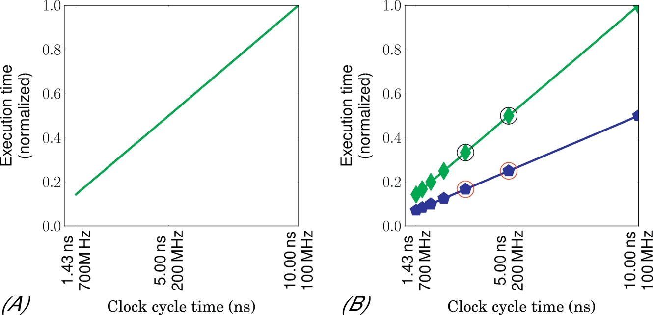
Existing DVFS performance models are primarily aimed at the CPU. They each exploit some kind of linear model, based on the fact that CPU computation scales with frequency speed while memory latency does not. These models fall into four classes: (a) proportional, (b) sampling, (c) empirical, and (d) analytical. The proportional scaling model assumes a linear relation between the performance and the core clock frequency (Fig. 3A). The sampling model better accounts for memory effects by identifying a scaling factor (ie, slope) for each application from two different voltage-frequency operating points. For example in Fig. 3B, we have two different slopes for two applications. The empirical model approximates that slope by counting aggregate performance counter events, such as the number of memory accesses. This model cannot distinguish between applications with low or high memory-level parallelism (MLP) [33].
An analytical model views a program as an alternating sequence of compute and memory phases. In a compute phase, the core executes useful instructions without generating any memory requests (eg, instruction fetches, data loads) that reach main memory. A memory request that misses the last level cache might trigger a memory phase, but only when a resource is exhausted and the pipeline stalls. Once the instruction or data access returns, the core typically begins a new compute phase. In all the current analytical models, the execution time (T) of a program at a voltage-frequency setting with cycle time t is expressed as
They strictly assume that the pipeline portion of the execution time (TCompute) scales with the frequency, while the nonpipeline portion (TMemory) does not. The execution time at an unexplored voltage-frequency setting of v2, f2 can be estimated from the measurement in the current settings v1, f1 by
The accuracy of these models relies heavily on accurate classification of cycles into compute or memory phase cycles, and this is the primary way in which these models differ. We describe them next.
Stall time
Stall time [35] estimates the nonpipeline phase (TMemory) as the number of cycles the core is unable to retire any instructions due to outstanding last level cache misses. It ignores computation performed during the miss before the pipeline stall. Since the scaling of this portion of computation can be hidden under memory latency, stall time overpredicts execution time.
Miss model
The Miss model [35] includes reorder buffer (ROB) fill time inside the memory phase. It identifies all the stand-alone misses, but only the first miss in a group of overlapped misses as a contributor to TMemory. In particular, it ignores misses that occur within the memory latency of an initial miss. The resulting miss count is then multiplied by a fixed memory latency to compute TMemory. This approach loses accuracy due to its fixed latency assumption and also ignores stall cycles due to instruction cache misses.
Leading load
Leading load [33, 36] recognizes both front-end stalls due to instruction cache misses and back-end stalls due to load misses. Their model counts the cycles when an instruction cache miss occurs in the last level cache. It adopts a similar approach to the miss model to address MLP for data loads. However, to account for variable memory latency, it counts the actual number of cycles a contributor load is outstanding.
Critical path
Critical path [34] computes TMemory as the longest serial chain of memory requests that stalls the processor. The proposed counter architecture maintains a global critical path counter (CRIT) and a critical path time stamp register (τi) for each outstanding load i. When a miss occurs in the last level cache (instruction or data), the snapshot of the global critical path counter is copied into the load’s time stamp register. Once the load i returns from memory, the global critical path counter is updated with the maximum of CRIT and τi + Li, where Li is the memory latency for load i.
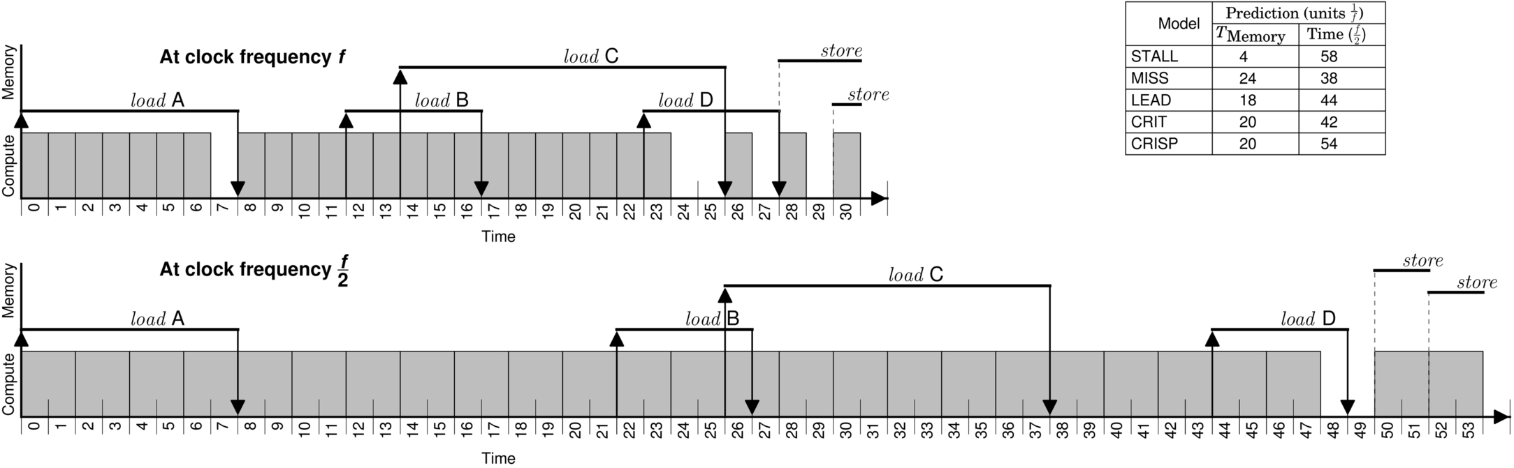
Example
Fig. 4 provides an example of a CPU program that has one stand-alone load miss (A at cycle 0) and two overlapped load misses (B at cycle 12 and C at cycle 14). At clock frequency f, the core stalls between cycles 1–7 and 15–25 for the loads to complete. The total execution time of the program at clock frequency f is 33 units (18 units stalls + 15 units computation). As we scale down the frequency to ![]() , the compute cycles (0, 8–14, 26–32) scale by a factor of 2. However, the expansion of compute cycles at 0 and 14 are hidden by the loads A and C, respectively. Thus the execution time at frequency
, the compute cycles (0, 8–14, 26–32) scale by a factor of 2. However, the expansion of compute cycles at 0 and 14 are hidden by the loads A and C, respectively. Thus the execution time at frequency ![]() becomes 46 units.
becomes 46 units.
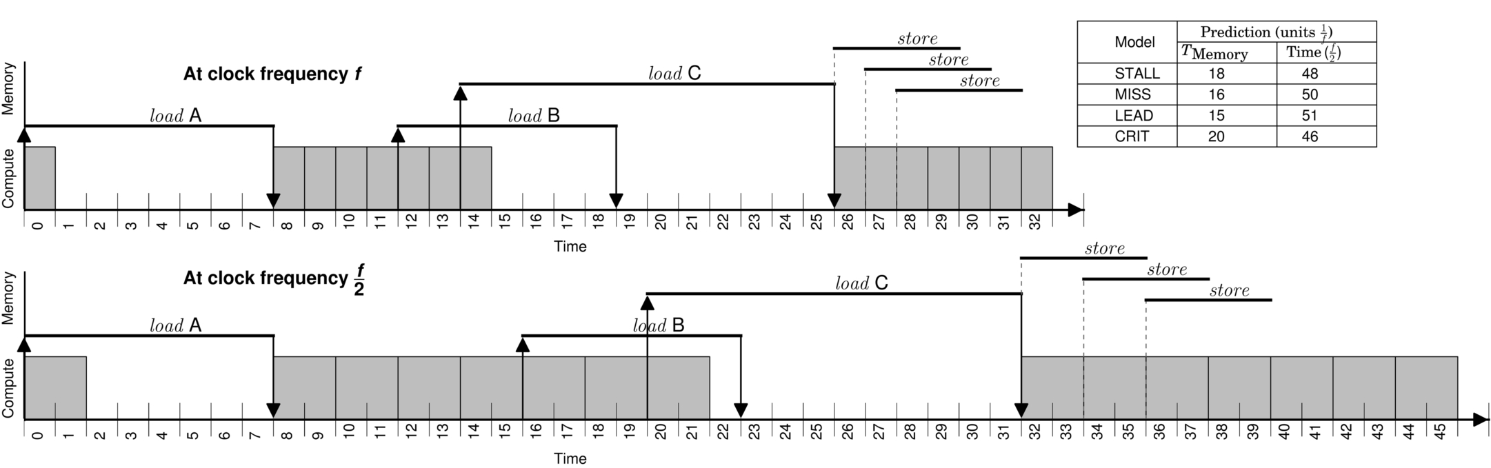
For each performance model, we identify the cycles classified as the nonpipelined (does not scale with the frequency of the pipeline) portion of computation. Leading load (LEAD) computes TMemory as the sum of A and B’s latencies (7 + 8 = 15). Miss model (MISS) identifies two contributor misses (A and B) and reports TMemory to be 16 (8 × 2). Among two dependent load paths (A + B with length 8 + 7 = 15, A + C with length 8 + 12 = 20), critical path (CRIT) selects A + C as the longest chain of dependent memory requests and computes the critical path as 20. Stall time (STALL) counts the 18 cycles of load-related stalls.
We plug in the value of TMemory in Eq. (2) and predict the execution time at clock frequency ![]() . The predicted execution time by the different models is shown in Fig. 4. Note that the models also differ in their counting of TCompute. Critical path (CRIT) outperforms the other models in this example. Although these models show reasonable accuracy in CPUs, optimization techniques like software and hardware prefetching may introduce significant overlap between computation and memory load latency, and thus invalidate the nonelasticity assumption of the memory component. In that case, the CRISP model should also provide significant improvement for CPU performance prediction.
. The predicted execution time by the different models is shown in Fig. 4. Note that the models also differ in their counting of TCompute. Critical path (CRIT) outperforms the other models in this example. Although these models show reasonable accuracy in CPUs, optimization techniques like software and hardware prefetching may introduce significant overlap between computation and memory load latency, and thus invalidate the nonelasticity assumption of the memory component. In that case, the CRISP model should also provide significant improvement for CPU performance prediction.
2.2 DVFS in GPGPUs
To explore the applicability of DVFS in GPGPUs, we simulate a NVIDIA Fermi architecture using GPGPU-Sim [37] and run nine kernels from the Rodinia [38] benchmark suite at different core clock frequencies—from 700 MHz (baseline) to 100 MHz (minimum). The performance curve in Fig. 5 shows the increase in runtime as we scale down the core frequency, that is, increase clock cycle time (x-axis). We make two major observations from this graph. First, like CPUs, there is significant opportunity for DVFS in GPUs—we see this because two of the kernels (cfd and km) are memory bound and insensitive to frequency changes (they have a flat slope in this graph), while three others (ge, lm, and hw) are only partially sensitive. For the memory-bound kernels, it is possible to reduce clock frequency and thus save energy without any performance overhead.
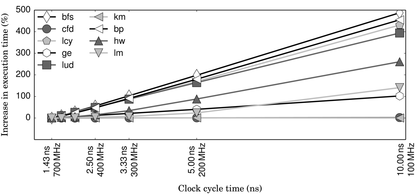
Our second observation is that the linear assumption of all prior models does not strictly hold because the partially sensitive kernels (eg, lm and hw) seem to follow two different slopes, depending on the frequency range. At high frequency, they follow a flat slope, as if they were memory bound (eg, between 700 and 300 MHz in lm), but at lower frequencies, they scale like compute-bound applications (eg, below 300 MHz in lm).
So while several of the principles that govern DVFS in CPUs also apply to GPUs, we identify several differences that make the existing models inadequate for GPUs. All of these differences stem from the high thread-level parallelism in GPU cores, resulting from the SIMT parallelism enabled through warp scheduling. The first difference is the much higher incidence of overlapped computation and memory access. The second is the homogeneity of computation in SIMT scheduling, resulting in the easy saturation of resources like the store queue. The third is the difficulty of classifying stalls (eg, an idle cycle may occur when five warps are stalled for memory and three are stalled for floating-point RAW hazards). We will discuss each of these differences, as well as a fourth that is more of an architectural detail and easily handled.
Memory/computation overlap
Existing models treat computation that happens in series with memory access the same as computation that happens in parallel. When the latter is infrequent, those models are fairly accurate, but in a GPGPU with high thread-level parallelism, it is common to find significant computation that overlaps with memory.
This overlapped computation has more complex behavior than the nonoverlapped. In the top timeline in Fig. 4 the computation at cycle 0 is overlapped with memory, so even though it is elongated, it still does not impact execution time, thus that computation looks more like memory than computation. However, if we extend the clock enough (ie, more than a factor of 8 in this example), that computation completely covers the memory latency and then begins to impact total execution time, now looking like computation again. This phenomenon exactly explains the two-slope behavior exhibited by hw and lm in Fig. 5.
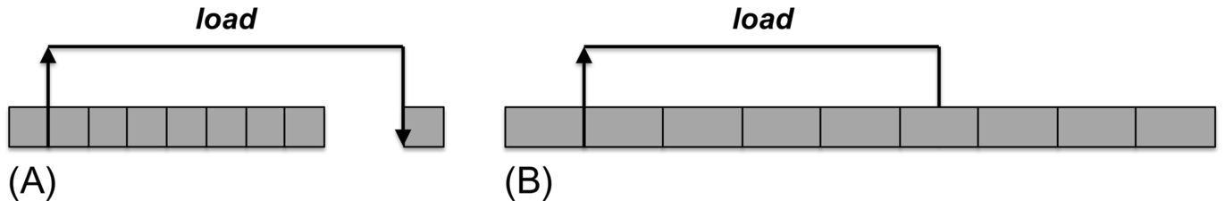
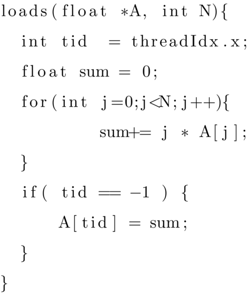
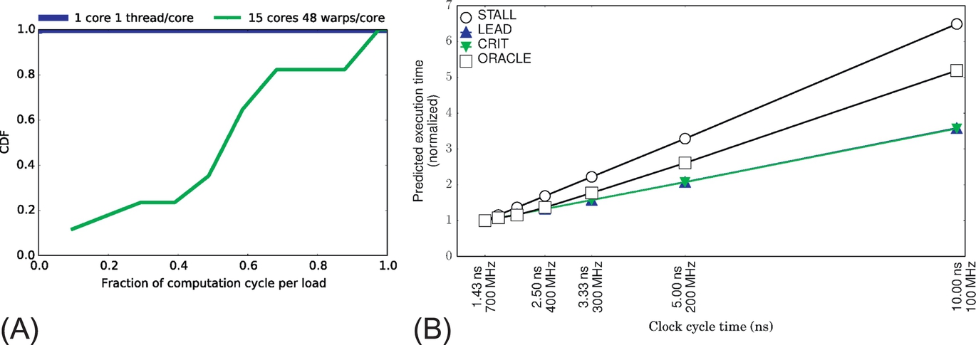
To examine this phenomenon more closely, we use the “load micro kernel” in Fig. 6 and run it for both single-threaded and many-threaded configurations. The cumulative distribution function shown in Fig. 7A shows that the single-threaded version has nearly zero computation-memory overlap. However, for the many-threaded version, more than 60% of loads have at least 50% of their cycles that are overlapped with computation. When we use the current performance models to predict the execution time of the many-threaded load kernel, the best ones (STALL, CRIT) underpredict execution time severely by ignoring the scaling of overlapped computation (Fig. 7B).
Store stalls
A core (CPU or GPU) will stall for a store only when the store queue fills, forcing it to stall and wait for one of the stores to complete. While this is a rare occurrence in CPUs, in a GPU with SIMT parallelism, it is common for all of the threads to execute stores at once, easily flooding the store queue, resulting in memory stalls that do not scale with frequency.
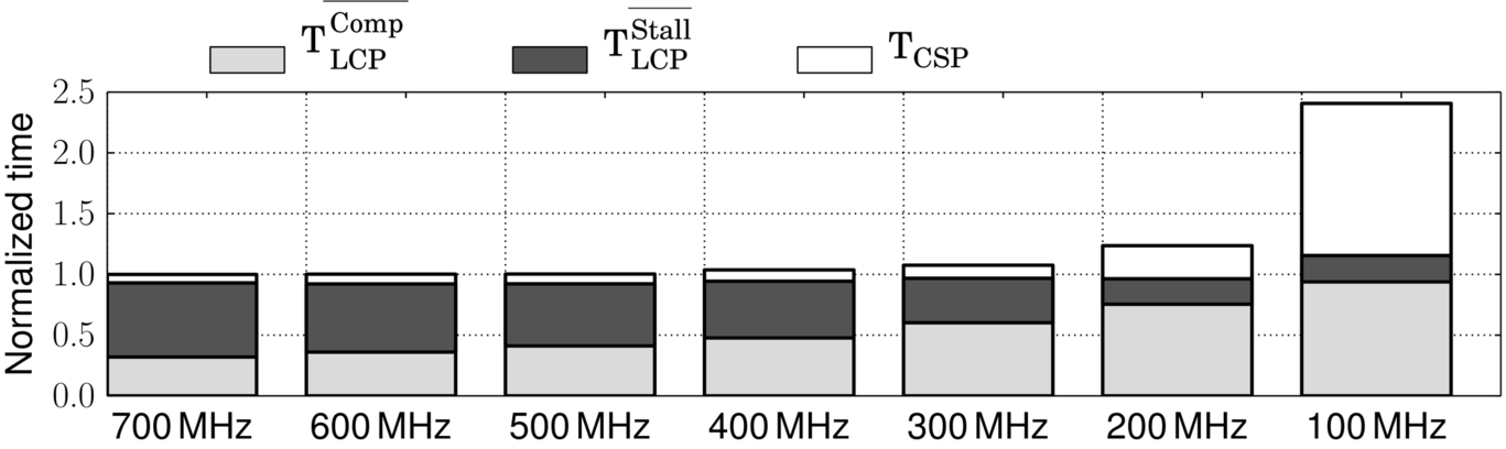
The “store micro kernel” in Fig. 8 initializes an array with constant values. In this code, the SIMD store instruction may fork into 32 individual stores, which can overload the load-store queue (LSQ) unit very quickly. As we increase the amount of parallelism by increasing the number of threads and warps, the percentage of cycles when the LSQ is full increases (Table 1) sharply. The prediction accuracy of the existing analytical models also decreases as we increase parallelism. As illustrated in Fig. 9A, the single-threaded configuration of the store micro kernel is fully compute bound with a very steep slope. Since there is no store-related stall, LEAD and CRIT predict execution time correctly for this configuration. However, for other configurations (Fig. 9B and C) that actually exhibit store stalls, the existing models treat the store stalls the same as computation and overpredict execution time.
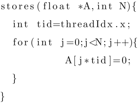
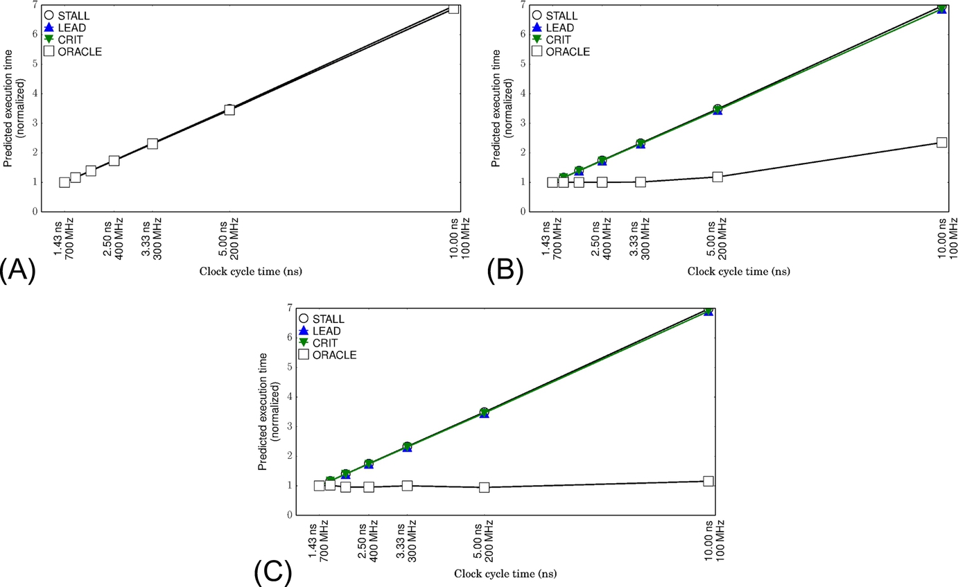
Table 1
Percentage of Cycles When Load-Store Queue Unit Is Full
| Parallelism | Cycle (%) |
| 1 Thread × 1 core | 0 |
| 1 Warp × 1 core | 66 |
| 8 Warps × 15 cores | 96 |
We observe an interesting two-phase behavior of the one-warp version of the store kernel in Fig. 9B. The kernel behaves as though it is memory bound in the high-frequency range and compute bound in the low-frequency range. As we decrease the core clock frequency, the stalls also decrease because of the LSQ being full. In fact, the store-related stall cycles act as idle cycles that can be converted to computation in a lower frequency. Once the frequency is low enough that all of the store stalls disappear (are covered by computation), the kernel then exhibits fully compute-bound behavior.
Complex stall classification
Identifying the cause of a stall cycle is difficult in the presence of high thread-level parallelism. For example, if several threads are stalled waiting for memory, but a few others are stalled waiting for floating-point operations to complete, is this a computation or memory phase? Prior works (which start counting memory cycles only after the pipeline stalls) would categorize this as computation because the pipeline is not yet fully stalled for memory, and the ongoing floating-point operations will scale with frequency.
Consider what happens when, as described earlier, the overlapped computation is scaled to the point where it completely covers the memory latency and now starts to interfere with other computation. The originally idle cycles (eg, between dependent floating-point ops) will not contribute to extending execution time, but rather will now be interleaved with the other computation. Only the cycles where the pipeline was actually issuing instructions will impact execution time. Thus, unlike other models, we generally treat mixed-cause idle cycles (both memory and CPU RAW hazards) as memory cycles rather than computation cycles.
L1 cache miss
A substantial portion of memory latency in a typical GPGPU is due to the interconnect that bridges the streaming cores to L2 cache and GPU global memory. The leading load and critical path models start counting cycles as the load request misses the last level cache, which works for CPUs where all on-chip caches are clocked together; however, in our GPU the interconnect and last level cache are in an independent clock domain.
Since this is not a shortcoming in the models, just a change in the assumed architecture, we adapt these models (as well as our own) to begin counting memory stalls as soon as they miss the L1 cache. This results in significantly improved accuracy for those models on GPUs. Thus all results shown in this chapter for leading load and critical path incorporate that improvement.
2.3 Models for GPGPUs
A handful of power and energy models have recently been proposed for GPGPUs [18]. However, very few of these models involve performance predictions. Dao et al. [39] propose linear and machine-learning-based models to estimate the runtime of kernels based on workload distribution. The integrated GPU power and performance (IPP) [40] model predicts the optimum number of cores for a GPGPU kernel to reduce power. However, they do not address the effect of clock frequency on GPU performance. Moreover, they ignore cache misses [41], which is critical for a DVFS model. Song et al. [42] contribute a similar model for a distributed system with GPGPU accelerators. Chen et al. [43] track NBTI-induced threshold voltage shift in GPGPU cores and determine the optimum number of cores by extending IPP. Equalizer [44] maintains performance counters to classify kernels as compute-intensive, memory-intensive, or cache-sensitive, using those classifications to change thread counts or P-States. However, because they have no actual model to predict performance, it still amounts to a sampling-based search for the right DVFS state.
None of these models address the effect of core clock frequency on kernel performance. CRISP is unique in that it is the first runtime analytical model, either for CPUs or GPGPUs, to model the nonlinear effect of frequency on performance—this effect can be seen in either system, but is just more prevalent on GPGPUs.
The only GPU analytical model that accounts for frequency is an empirical model [45] that builds a unique nonlinear performance model for each workload—this is intended to be used offline and is not practical for an online implementation. Abe et al. [14, 15] also present an offline solution. They use a multiple linear regression-based approach with higher average prediction error (40%). Their maximum error is more than 100%.
3 GPGPU DVFS performance model
This section describes the CRISP performance predictor, a novel analytical model for predicting the performance impact of DVFS in modern many-core architectures like GPGPUs.
3.1 Critical Stalled Path
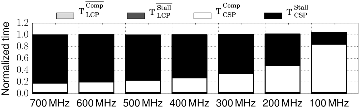
Our model interprets computation in a GPGPU as a collection of three distinct phases: load outstanding, pure compute, and store stall (Fig. 10). The core remains in a pure compute phase in the absence of an outstanding load or any store-related stall. Once a fetch or load miss occurs in one of the level 1 caches (constant, data, instruction, texture), the core enters a load outstanding phase and stays there as long as a miss is outstanding. During this phase, the core may schedule instructions or stall due to control, data, or structural hazards. The store stall phase represents the idle cycles due to store operations, in the explicit case where the pipeline is stalled due to store queue saturation.
We split the total computation time into two disjoint segments: a load critical path (LCP) and a compute/store path (CSP).
This division allows us to separately analyze (1) loads and the computation that competes with loads to become performance-critical versus (2) computation that never overlaps loads and is exposed regardless of the behavior of the loads. Store stalls fall into the latter category because any cycle that stalls in the presence of both loads and stores is counted as a load stall.
The LCP is the length of the longest sequence of dependent memory loads (possibly overlapped with computation) from parallel warps. Thus it does not necessarily include all loads, which enables it to account for MLP by not counting loads that occur in parallel, similar to Ref. [33, 34]. Meanwhile, we form the CSP as a summation of nonoverlapped compute phases, store stall phases, and computation overlapped only by loads not deemed part of the critical path. Since the two segments in Eq. (3) scale differently with core clock frequency, we develop separate models for each.
3.2 LCP Portion
SMs have high thread-level parallelism. The maximum number of concurrently running warps per SM varies from 24 to 64 depending on the compute capability of the device (eg, 48 in the NVIDIA Fermi architecture). This enables the SM to hide significant amounts of memory latency, resulting in heavy overlap between load latency and useful computation. However, it often does not hide all of it, due to lack of parallelism (either caused by low inherent parallelism or restricted parallelism due to resource constraints) or poor locality.
We represent the LCP as a combination of memory-related overlapped stalls (![]() ) and overlapped computations (
) and overlapped computations (![]() ). Prior CPU-based models’ assumption of TMemory’s inelasticity creates a larger inaccuracy in GPGPUs than it does for CPUs because of the magnitude of
). Prior CPU-based models’ assumption of TMemory’s inelasticity creates a larger inaccuracy in GPGPUs than it does for CPUs because of the magnitude of ![]() , which scales linearly with frequency. The expansion of overlapped computation stays hidden under TMemory as long as the frequency scaling factor is less than the ratio between TMemory and the overlapped computation. As the frequency is scaled further, the LCP can be dominated by the length of the scaled overlapped computation. Thus we define the LCP portion of the model as
, which scales linearly with frequency. The expansion of overlapped computation stays hidden under TMemory as long as the frequency scaling factor is less than the ratio between TMemory and the overlapped computation. As the frequency is scaled further, the LCP can be dominated by the length of the scaled overlapped computation. Thus we define the LCP portion of the model as
We describe details on parameterizing this equation from hardware events in Sections 3.5 and 3.6. Fig. 11 shows the normalized execution time of the lm kernel for seven different frequencies. As expected, we see the load stalls decreasing with lower frequency, but without increasing total execution time for small changes in frequency. As the frequency is decreased further, the overlapped computation increases, with much of it turning into nonoverlapped computation (as some of the original overlapped computation now extends past the duration of the load), resulting in an increase in total execution time. Prior models assume that overlapped computation always remains overlapped, and miss this effect.
3.3 Compute/Store Path Portion
The compute/store critical path includes computation (TCSPComp) that is not overlapped with memory operations and simply scales with frequency, plus store stalls (TCSPStall). SMs have a wide SIMD unit (eg, 32 in Fermi). A SIMD store instruction may result in 32 individual scalar memory store operations if uncoalesced (eg, A[tid * 64] = 0). As a result, the LSQ may overflow very quickly during a store-dominant phase in the running kernel. Eventually, the level 1 cache runs out of miss status holding register (MSHR) entries, and the instruction scheduler stalls due to the scarcity of free entries in the LSQ or MSHR. We observe this phenomenon in several of our application kernels, as well as microbenchmarks we used to fine-tune our models. Again, this is a rare case for CPUs, but easily generated on an SIMD core. Although the store stalls are memory delays, they do not remain static as frequency changes. As frequency slows, the rate (as seen by the memory hierarchy) of the store generation slows, making it easier for the LSQ and the memory hierarchy to keep up. A simple model (meaning one that requires minimal hardware to track) that works extremely well empirically assumes that the frequency of stores decreases in response to the slowdown of nonoverlapped computation (recall, the overlapped computation may also generate stores, but those stores do not contribute to the stall being considered here). Thus we express the CSP by the following equation in the presence of DVFS.
We see this phenomenon, but only slightly, in Fig. 11, but much more clearly in Fig. 12, which shows one particular store-bound kernel in cfd. As frequency decreases, computation expands but does not actually increase total execution time; it only decreases the contribution of store stalls.
We assume that the stretched overlapped computation and the pure computation will serialize at a lower frequency. This is a simplification, and a portion of CRISP’s prediction error stems from this assumption. This was a conscious choice to trade accuracy for complexity, because tracking those dependencies between instructions is another level of complexity and tracking.
In summary, then, CRISP divides all cycles into four distinct categories: (1) pure computation, which is completely elastic with frequency, (2) load stall, which as part of the LCP is inelastic with frequency, (3) overlapped computation, which is elastic, but potentially hidden by the LCP, and (4) store stall, which tends to disappear as the pure computation stretches.
3.4 Example
We illustrate the mechanism of our model in Fig. 13 where loads and computations are from all the concurrently running warps in a single SM. The total execution time of the program at clock frequency f is 31 units (5 units stall + 26 units computation). As we scale down the frequency to ![]() , all the compute cycles scale by a factor of 2. Because of the scaling of overlapped computation under load A (cycles 0–6) at clock frequency
, all the compute cycles scale by a factor of 2. Because of the scaling of overlapped computation under load A (cycles 0–6) at clock frequency ![]() , the compute cycle 8 cannot begin before time unit 14. Similarly, the instruction at compute cycle 28 cannot be issued until time unit 50 because the expansion of overlapped computation under load C (cycles 14–23) pushes it further. Meanwhile, as the computation at cycle 28 expands due to frequency scaling, it overlaps with the subsequent store stalls.
, the compute cycle 8 cannot begin before time unit 14. Similarly, the instruction at compute cycle 28 cannot be issued until time unit 50 because the expansion of overlapped computation under load C (cycles 14–23) pushes it further. Meanwhile, as the computation at cycle 28 expands due to frequency scaling, it overlaps with the subsequent store stalls.
For each of the prior performance models, we identify the cycles classified as the nonpipelined portion of computation (TMemory). Leading load (LEAD) computes TMemory as the sum of A, B, and D’s latencies (8 + 5 + 5 = 18). Miss model (MISS) identifies three contributor misses (A, B, and D) and reports TMemory to be 24 (8 × 3). Among two dependent load paths (A + B + D with length 8 + 5 + 5 = 18, A + C with length 8 + 12 = 20), CRISP computes the LCP as 20 (for the longest path A + C). The stall cycles computed by STALL are 4. We plug in the value of TMemory in Eq. (2) and predict the execution time at clock frequency ![]() . As expected, the presence of overlapped computation under TMemory and store-related stalls introduces an error in the prediction of the prior models. The STALL model overpredicts, while the rest of the models underpredict.
. As expected, the presence of overlapped computation under TMemory and store-related stalls introduces an error in the prediction of the prior models. The STALL model overpredicts, while the rest of the models underpredict.
Our model observes two load outstanding phases (cycles 0–7 and 12–27), three pure compute phases (cycles 8–11, 28, and 30), and one store stall phase (cycle 29). CRISP computes the LCP as 20 (8 + 12 for load A–C). The rest of the cycles (11 = 31 − 20) are assigned to the CSP. The overlapped computation under LCP is 17 (cycles 0–6 and 14–23). The nonoverlapped computation in CSP is 10 (cycles 8–13, 26–28, and 30). Note that cycle 29 is the only store stall cycle. CRISP computes the scaled LCP as max (17 × 2, 20) = 34 and CSP as max (10 × 2, 11) = 20. Finally, the predicted execution time by CRISP at clock frequency ![]() is 54 (34 + 20), which matches the actual execution time (54).
is 54 (34 + 20), which matches the actual execution time (54).
3.5 Parameterizing the Model
To utilize our model, the core needs to partition execution cycles along some fairly subtle distinctions, separating two types of computation cycles and two types of memory stalls, while accounting for the fact that, in a heavily multithreaded core, there are often a plethora of competing causes for each idle cycle.
Despite these issues, we are able to measure all of these parameters with some simple rules and a very small amount of hardware. First, we categorize each cycle as either one of two types of stalls (load stalls within the LCP or store stalls within the CSP) or computation. Next we split computation into overlapped computation (within the LCP) or nonoverlapped.
Identifying stalls
Memory hierarchy stalls can originate from instruction cache fetch misses, load misses, or store misses. The first two we categorize as load stalls and the last one only manifests in pipeline stalls when we run out of LSQ entries or MSHRs. We initially separate these two types of stalls from computation cycles and then will break down the computation cycles in the next section.
Identifying the cause of stall cycles in a heavily multithreaded core is less than straightforward. We assume the following information is available in the pipeline or L1 cache interface: the existence of outstanding load misses, the existence of outstanding store misses, the existence of a fetch stall in the front-end pipeline, MSHR or LSQ full condition, and the existence of RAW hazard on a memory operation, a RAW hazard on an arithmetic operation causing an instruction to stall, or an arithmetic structural hazard. Most of those are readily available in any pipeline, but the last three might each require an extra bit of storage and some minimal logic added to the GPU scoreboard.
Because our GPU can issue two instructions (two arithmetic or one arithmetic and one load/store), characterizing cycles as idle or busy is already a bit fuzzy. Two-issue cycles are busy (computation), zero-issue cycles are considered idle. On the other hand, one-issue cycles will be counted as busy if there is an arithmetic RAW or structural hazard; otherwise, they will be characterized as idle since there is a lack of sufficient arithmetic instructions to fully utilize the issue bandwidth.
Idle cycles will be characterized as load stalls, store stalls, or computation, according to the following algorithm, the order of which determines the characterization of stalls in the presence of multiple potential causes:
(A) If there is a control hazard (branch mispredict), cache/shared memory bank conflict, or no outstanding load or store misses or fetch stall, this cycle is counted as computation. Branch mispredicts are resolved at the speed of the pipeline, as are L1 cache and shared memory bank conflicts (L1 cache and shared memory run on the same clock as the pipeline).
(B) Else, if there is an outstanding load miss, then if there is a RAW hazard on the load/store unit, this cycle is a load stall. Otherwise, if there is an arithmetic RAW or structural hazard, then this cycle is computation. If neither is the case and the MSHR or LSQ are full, then this is a load stall. Finally, if there is a fetch stall in the front end, then it is a load stall.
(C) Else (no outstanding load miss), then if the MSHR or LSQ are full, this indicates a store stall.
(D) All other stalls must be solely due to arithmetic dependencies and are classified as computation.
Classifying computation
After identifying the total cycles of computation, we divide those into two groups: the pure computation that is part of the CSP and the overlapped computation that is overlapped by the LCP. The former includes both computation that does not overlap loads and computation that overlaps loads that are not part of the critical path. The reason for dividing computation into these sets is that the compute/store computation is always exposed (execution time is sensitive to their latency) while the latter become exposed only when they exceed the load stalls. We describe the mechanism to compute the computation under the LCP here, but revisit the need to precisely track the critical path in Section 3.4.
In order to track the computation that is overlapped by the LCP, we need to track the critical path using a mechanism similar to the critical path model [34]. This is done using a counter to track the global longest critical path (the current TMemory up to this point), as well as counters for each outstanding load that record the critical path length when they started, so that we can decide when they finish if they extend the global longest critical path. However, we instead measure something we call the adjusted LCP, which adds load stalls as one-cycle additions to the running global longest critical path. In this way, when the longest critical path is calculated, its length will include both the critical path load latencies and the stalls that lie between the critical loads—the noncritical load stalls. That adjusted LCP is the TLCP(t) from Eq. (3), which is also the “LCP” from Fig. 10 and includes all load stalls (either as part of the critical load latencies or the noncritical stalls) as well as all overlapped computation. As a result, we can solve for the overlapped computation simply by subtracting the total load stalls from the adjusted LCP; this is possible because we also record the total load stalls in a counter.
In the top timeline in Fig. 13, the original critical path computation will count 8 (latency of A) + 12 (latency of C) = 20 cycles as the LCP, but our adjusted LCP will also pick up the stall at cycle 27 and will calculate 21 as our adjusted LCP. At the same time, we count 4 total load stall cycles. Subtracting 4 from 21 gives us 17 cycles of load-critical overlapped computation, which is exactly the number of computation cycles under the two critical path loads (A and C).
3.6 Hardware Mechanism and Overhead
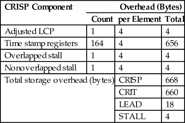
We now describe the hardware mechanisms that enable CRISP. It maintains three counters: adjusted LCP (TMemory), load stall (![]() ), and store stall (TCSPStall). The rest of the terms in Eqs. (3), (4) can be computed from these three counters and total time by simple subtraction. Like the original critical path (CRIT) model, it also maintains a critical path time stamp register (tsi) for each outstanding miss (i) in the L1 caches (one per MSHR). Table 2 shows the total hardware overhead for these counters, 99% of which is inherited from CRIT. We discuss the software overhead in Section 5.
), and store stall (TCSPStall). The rest of the terms in Eqs. (3), (4) can be computed from these three counters and total time by simple subtraction. Like the original critical path (CRIT) model, it also maintains a critical path time stamp register (tsi) for each outstanding miss (i) in the L1 caches (one per MSHR). Table 2 shows the total hardware overhead for these counters, 99% of which is inherited from CRIT. We discuss the software overhead in Section 5.
Table 2
Hardware Storage Overhead per SM of CRISP
| CRISP Component | Overhead (Bytes) | ||
| Count | per Element | Total | |
| Adjusted LCP | 1 | 4 | 4 |
| Time stamp registers | 164 | 4 | 656 |
| Overlapped stall | 1 | 4 | 4 |
| Nonoverlapped stall | 1 | 4 | 4 |
| Total storage overhead (bytes) | CRISP | 668 | |
| CRIT | 660 | ||
| LEAD | 18 | ||
| STALL | 4 | ||
At the beginning of each kernel execution, the counters are set to zero. Once a load request i (instruction, data, constant, or texture) misses in the level 1 cache, CRISP copies TMemory into the pending load’s time stamp register (tsi). When the load i’s data is serviced from the L2 cache or memory after Li cycles, TMemory is updated with the maximum of TMemory and tsi + Li. In the occurrence of a load stall, CRISP increments TMemory and ![]() . For each nonoverlapped (store) stall, CRISP increments TCSPStall.
. For each nonoverlapped (store) stall, CRISP increments TCSPStall.
An unoptimized implementation of the logic that detects load and store stall needs just 12 logic gates and is never on the critical path. Most of the signals used in the cycle classification logic are already available in current pipelines. To detect different kinds of hazards, we alter the GPU scoreboard, which requires 1 bit per warp in the GPU hardware scheduler and minimal logic.
4 Methodology
CRISP, like other existing online analytical models, requires specific changes in hardware. As a result, we rely on simulation (specifically, the GPGPU-Sim [37] simulator) to evaluate the benefit of our novel performance model, as in prior work (CRIT [34], LEAD [33, 36]). The GPGPU configuration used in our experiment (Table 3) is very similar to the NVIDIA GTX 480 Fermi architecture (in Section 5.4, we also evaluate a Tesla C2050). To evaluate the energy savings realized by CRISP, we update the original GPGPU-Sim with online DVFS capability. All the 15 SMs in our configured architecture share a single voltage domain with a nominal clock frequency of 700 MHz. We define six other performance states (P-State) for the SMs, ranging from 100 to 600 MHz with a step size of 100 MHz [18]. Similar to GPUWattch [18], we select the voltage for each P-State from 0.55 to 1.0 V. We rely on a fast-responding on-chip global DVFS regulator that can switch between P-States in 100 ns [18, 46–48]. We account for this switching overhead for each P-State transition in our energy savings result.
Table 3
GPGPU Configuration
| SM | Memory | Cache | Clock Frequency | ||||||||
| Register | 32K | Size | 2 GB | L1 | Domain | MHz | |||||
| SP unit | 32 | Partition | 6 | Feature | Inst | Data | Const | Text | L2 | SM | 700 |
| SFU unit | 16 | Subpartition | 12 | Size (KB) | 2 | 16 | 8 | 12 | 786 | L2 cache | 700 |
| LD/ST unit | 16 | Scheduling | FRFCFS | Set | 4 | 32 | 64 | 4 | 64 | Memory | 1848 |
| Max CTA | 8 | Queue size | 16 | Assoc | 4 | 4 | 2 | 24 | 8 | Interconnect | 700 |
| Warp size | 32 | Bus width | 4 | MSHR | 2 | 32 | 2 | 128 | 32 | ||
| Max warp | 48 | Burst length | 8 | Line size | 128 | 128 | 64 | 128 | 128 | ||
| Max thread | 1536 | Controller | 6 | Replacement | LRU | LRU | LRU | LRU | LRU | ||
| Two warp scheduler | Write policy | RO | LWBGWT | RO | RO | WB | |||||
| Greedy then oldest | WA policy | NWA | NWA | NWA | NWA | WA | |||||
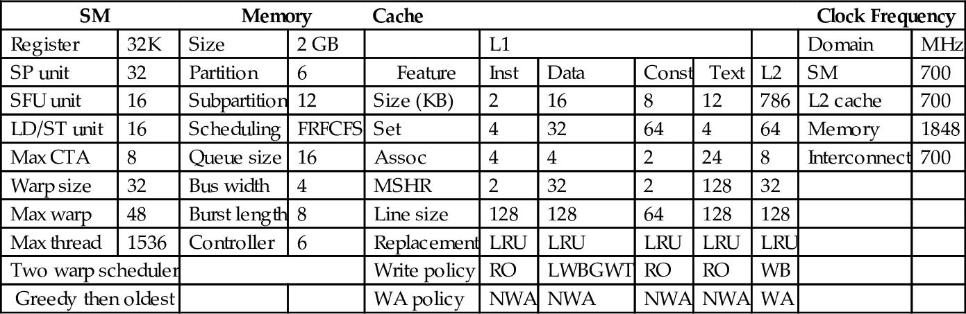
Notes: LWBGWT, local write back global write through; RO, read only; WA, write allocate.
We extend the GPUWattch [18] power simulator in GPGPU-Sim to estimate accurate power consumption in the presence of online DVFS. For each power calculation interval of GPUWattch, we collect the dynamic power at the nominal voltage-frequency (700 MHz, 1 V) setting and scale it for the current voltage-frequency (![]() ). We use GPUSimpow [49] to estimate the static power of individual clock domains at nominal frequency, which is between 23% to 63% for the Rodinia benchmark suite. The static power in other P-States are estimated using voltage scaling (
). We use GPUSimpow [49] to estimate the static power of individual clock domains at nominal frequency, which is between 23% to 63% for the Rodinia benchmark suite. The static power in other P-States are estimated using voltage scaling (![]() ) [50].
) [50].
We use the Rodinia [38] benchmark suite in our experiments. To initially assess the accuracy of different models, we run the first important kernel of each Rodinia benchmark for 4.8 million instructions—we exclude nw because the runtime of each kernel is smaller than a single reasonable DVFS interval. The 4.8 million-instruction execution of each kernel at nominal frequency translates into at least 10 μs execution time (ranging from 10 to 600 μs). We find that 10 μs is the minimum DVFS interval for which the switching overhead (100 ns) of the on-chip regulator is negligible (≤1%). Meanwhile, to evaluate the energy savings, we run the benchmarks for at least 1 billion instructions (except for myc, which we ran long enough to get 4286 full kernel executions). For some benchmarks, we ran for up to 9 billion instructions if that allowed us to run to completion. Eight of the benchmarks finish execution within that allotment. For presentation purposes, we divide the benchmarks into two groups. The benchmarks (bp, hw, hs, and patf) with at least 75% computation cycles are classified as compute bound. The rest of the benchmarks are memory-bound.
In Section 5.2, we demonstrate an application of our performance model in an online energy saving framework. In order to make decisions about DVFS settings to optimize EDP or similar metrics, we need both a performance model and an energy model. The energy model we use assumes that the phase of the next interval will be computationally similar to the current interval [34], which is typically a safe assumption for GPUs.
At each decision interval (10 μs), the DVFS controller uses the power model to find the static and dynamic power of the SMs at the current settings (vc, fc). It also collects static and dynamic power consumed by the rest of the components, including memory, interconnect, and level 2 cache. For each of the possible voltage-frequency settings (v, f), it predicts (a) static power of the SMs using voltage scaling, (b) dynamic power of the SMs using voltage and frequency scaling, and (c) execution time T(f) using the underlying DVFS performance model (leading load, stall time, critical path, or critical stalled path). The static and dynamic power of the rest of the system are assumed to remain unchanged since we do not apply DVFS to those domains.
The controller computes the total static energy consumption at each frequency f as a product of total static power PStatic(v, f) and T(f). Meanwhile, the total dynamic energy consumption at frequency f is computed as PDynamic(f) × T(fc). The static and dynamic energy components are added together to estimate the predicted energy E(f) at P-State (v, f). Finally, the controller computes ED2P (v, f) as E(f) × T(f)2 and makes a transition to the P-State with the predicted minimum ED2P. For the EDP operating setting, the controller orchestrates DVFS in similar fashion, with minimum EDP as the goal.
We measure the online software overhead at 109 cycles per decision interval by running the actual code on a CPU. Note that the same software could also run on an SM. This overhead is included in our modeled performance overhead, in addition to the 1% P-State switching overhead. It should be noted that we do not have any overhead for measurement because we do the measurement in the hardware using performance counters, except for reading the counters that are part of our software overhead.
In our results, we average performance-counter statistics across all SMs in the power domain to drive our performance model. However, our experiments (not shown here) demonstrate that we could instead sample a single core with no significant loss in effectiveness.
5 Results
This section examines the quality of the CRISP predictor in two ways. First, it evaluates the accuracy of the model in predicting kernel runtimes at different frequencies, compared to the prior state of the art. Second, it uses the predictor in a runtime algorithm to predict the optimal DVFS settings and measures the potential gains in energy efficiency. In each case we compare against leading load (LEAD), critical path (CRIT), and stall time (STALL). We also explore the performance of a computationally simpler version of CRISP. Last, we examine the generality of CRISP.
5.1 Execution Time Prediction
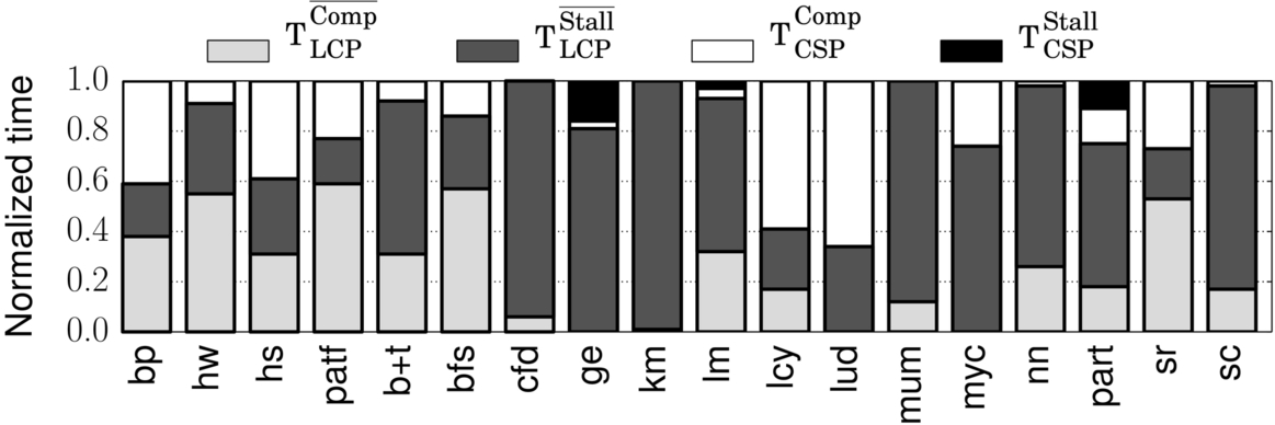
We simulate the first instance of a key kernel of each Rodinia [38] benchmark at all seven P-States and collect the execution time information at each frequency. We also save the performance model counter data at the nominal frequency (700 MHz) to drive the various performance models. We show the breakdown of the classifications computed by CRISP in Fig. 14; this raw data on each benchmark is useful in understanding some of the sources of prediction error. This data shows several interesting facts—(1) the benchmarks are diverse, (2) while the LCP often covers the majority of the execution time, the overlapped portion is often quite large, and (3) three of the kernels have noticeable nonoverlapped store stalls (TCSPStall).
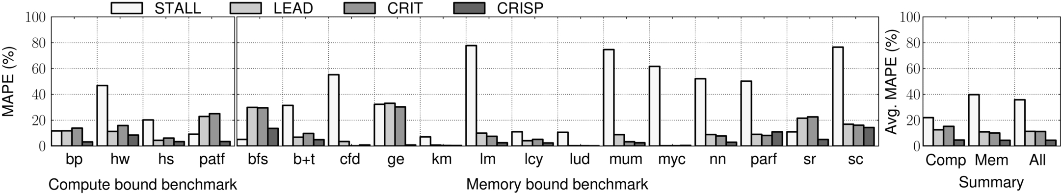
Based on the measured runtime and performance counter data at 700 MHz frequency, the performance models predict the execution time at six other frequencies (100–600 MHz). Fig. 15 shows the prediction error of each of the models for three target frequencies: 100, 400, and 600 MHz. We also highlight the mean absolute percentage error (MAPE) at these target frequencies in the rightmost graph of Fig. 15. The summarized average absolute percentage errors of the models across all six target frequencies for each benchmark are reported in Fig. 17.
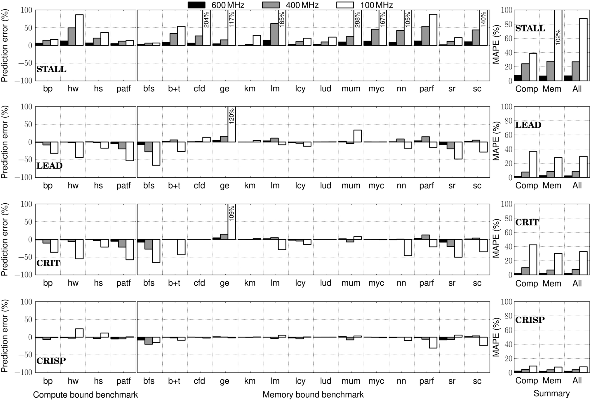
STALL always overpredicts the execution time, conservatively treating all stalls as completely inelastic. The inaccuracy of STALL can be as high as 288%. Both LEAD and CRIT suffer from underprediction (65% or more for bfs) and overprediction (109% or more for ge). The accuracy of CRISP also varies, but the maximum prediction error (30%) is reduced by a factor of 3.6 compared to the maximum error (109%) with the best of the existing models.
We see that both LEAD and CRIT are more prone to underpredicting the memory-bound kernels (those on the right side of the graph); this comes from their inability to detect when the kernels transition to computation-bound and become more sensitive to frequency. The major exception is ge, where they both fail to account for the store-related stalls and heavily over-predict execution time.
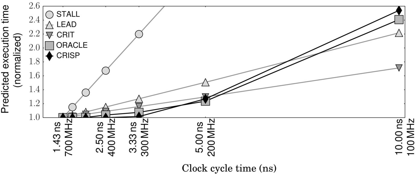
We also note from these results that as we try to predict the performance with a high scaling factor (from 700 to 100 MHz), the error of the prior techniques becomes superlinear—that is, they become proportionally more inaccurate the further you depart from the base frequency. The leading load paper acknowledges this. A big factor in this superlinear error is that the greater the change in frequency, the more likely it is that the load stalls are completely covered and the kernel transitions to a compute-bound scaling factor. This explains why the CRISP results do not appear to share the superlinear error, in general. To illustrate this, we show the predicted execution time for the lm kernel as we scale the frequency from 700 to 100 MHz (Fig. 16). CRIT measures TMemory as 0.88, while LEAD estimates it as 0.80. We measure the LCP length of lm to be 0.93 of which 34% are overlapped computations; thus we expect the LCP to be completely covered at about 233 MHz. We see that above this frequency CRIT is fairly accurate, but diverges widely after this point. Beyond this point, CRISP treats the kernel as completely compute-bound, while at 100 MHz CRIT is still assuming 52% of the execution time is spent waiting for memory. In contrast, CRISP closely follows the actual runtimes (ORACLE) both at memory-bound frequencies and at compute-bound frequencies.
We observe a similar phenomenon in the kernels hw, hs, and bfs. In each of these cases, CRISP successfully captures the piecewise linear behavior of performance under frequency scaling. As summarized in Fig. 17, the average prediction error of CRISP across all the benchmarks is 4% versus 11% with LEAD, 11% with CRIT, and 35% with STALL.
5.2 Energy Savings
An online performance model, and the underlying architecture to compute it, is a tool. An expected application of such a tool would be to evaluate multiple DVFS settings to optimize for particular performance and energy goals. In this section, we will evaluate the utility of CRISP in minimizing two widely used metrics: EDP and ED2P.
We compute the savings relative to the default mode, which always runs at maximum SM clock frequency (700 MHz, 1 V). We run two similar experiments with our simple DVFS controller (see Section 4) targeting (a) minimum EDP and (b) the minimum ED2P operating point. During both experiments, the controller uses the program’s behavior during the current interval to predict the next interval. We do the same for each of the other studied predictors—all use the same power predictor.
Using CRISP for this purpose does raise one concern. All of the models are asymmetric (ie, will predict differently for lower frequency A-¿B than for higher frequency B-¿A) due to different numbers of stall cycles, different loads on the critical path, and so on. However, the asymmetry is perhaps more clear with CRISP. While predicting for lower frequencies, we quite accurately predict when overlapped computation will be converted into pure computation; it is more difficult to predict which pure computation cycles will become overlapped computations at a higher frequency. We thus modify our predictor slightly when predicting for a higher frequency. We calculate the new execution time as ![]() . This ignores the possible expansion of store stalls and does not account for conversion of pure computation to overlapped. While this model will be less accurate, in a running system with DVFS (as in the next section), if it mistakenly forces a change to a higher frequency, the next interval will correct it with the accurate model. While this could cause ping-ponging, which we could solve with some hysteresis, we found this unnecessary.
. This ignores the possible expansion of store stalls and does not account for conversion of pure computation to overlapped. While this model will be less accurate, in a running system with DVFS (as in the next section), if it mistakenly forces a change to a higher frequency, the next interval will correct it with the accurate model. While this could cause ping-ponging, which we could solve with some hysteresis, we found this unnecessary.
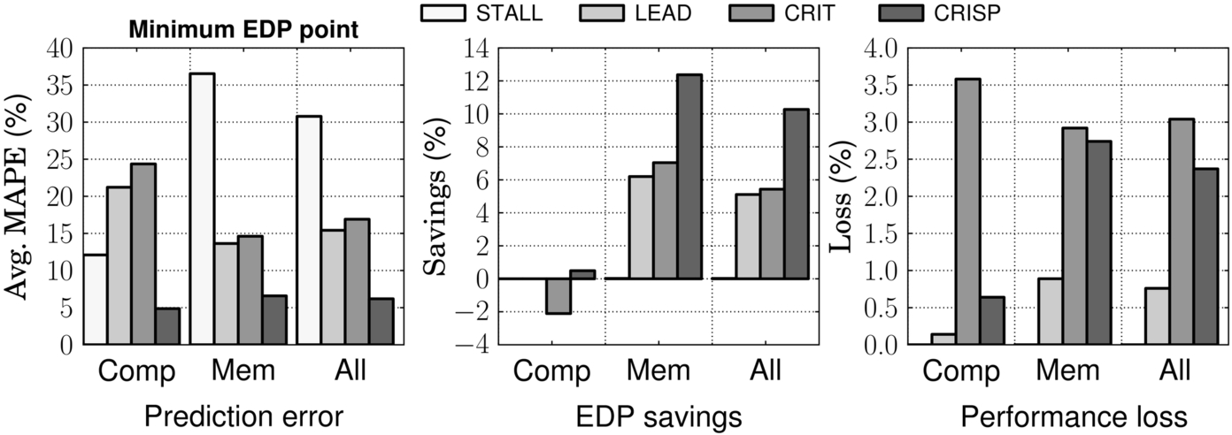
Optimizing for EDP
Fig. 18 shows EDP savings achieved by the evaluated performance models when the controller is seeking the minimum EDP point for each kernel. We included all the runtime overhead—software model computation and voltage switching overhead—in this result. For the 14 memory-bound benchmarks, CRISP reduces EDP by 13.9% compared to 8.9% with CRIT, 8.7% with LEAD, and 0% with STALL. CRISP achieves high savings in both lm (15.3%) and ge (21.8%). The other three models fail to realize any energy savings opportunity in lm and achieve very little savings (5% with CRIT and 1% with LEAD) in ge. As we saw previously in Fig. 16, CRISP accurately models lm at all frequency points. Thus it typically chooses to run this kernel at 300 MHz, resulting in 1.25% performance degradation but 16.4% reduced energy. CRIT and LEAD both overestimate the performance cost at this frequency and instead choose to run at 700 MHz.
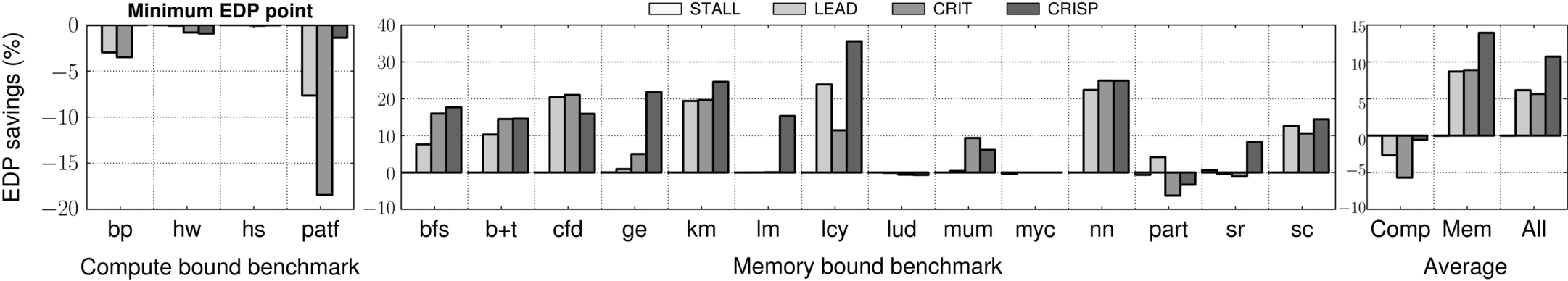
For the compute-bound benchmarks, CRISP marginally reduces EDP by 0.5%, while LEAD and CRIT increase EDP by 2.7% and 5.7%, respectively. Because of the underprediction of execution time (eg, patf), CRIT aggressively reduces the clock frequency and experiences 13.3% performance loss on average (33% in patf) for the compute bound benchmarks.
In summary, the average EDP savings for the Rodinia benchmark suite with CRISP is 10.7% versus 5.7% with CRIT, 6.2% with LEAD, and 0% with STALL. The selected EDP operating points of CRISP translate into 12.9% energy savings and 15.5% reduction in the average power with an average performance loss of 3.4%. CRIT saves 10.6% energy and LEAD saves 8.1%. The performance loss is 6.3% with CRIT and 2.9% with LEAD.
Optimizing for ED2P
When attempting to optimize for ED2P, CRISP again outperforms the other models by reducing ED2P 9.0% on average. The corresponding average savings realized by CRIT, LEAD, and STALL are only 3.5%, 4.9%, and 0%, respectively. Fig. 19 shows that the savings with CRISP is much higher (11.7%) for memory-bound benchmarks compared to CRIT (5.5%), LEAD (6.4%), and STALL (0%).
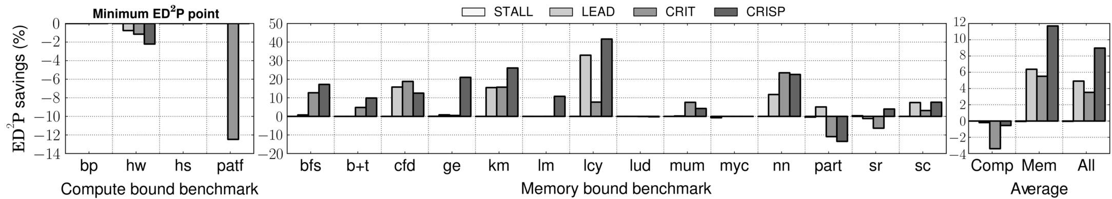
CRISP achieves its highest ED2P savings of 42% for lcy, by running the primary kernel at 500 MHz most of the time. CRIT and LEAD underpredict the energy saving opportunity and keep the frequency at 700 MHz for 50% and 41% of the duration of this kernel, respectively. As we analyze the execution trace, we find that 67% of cycles inside the LCP for that kernel are computation, thus are not handled accurately by the other models.
5.3 Simplified CRISP Model
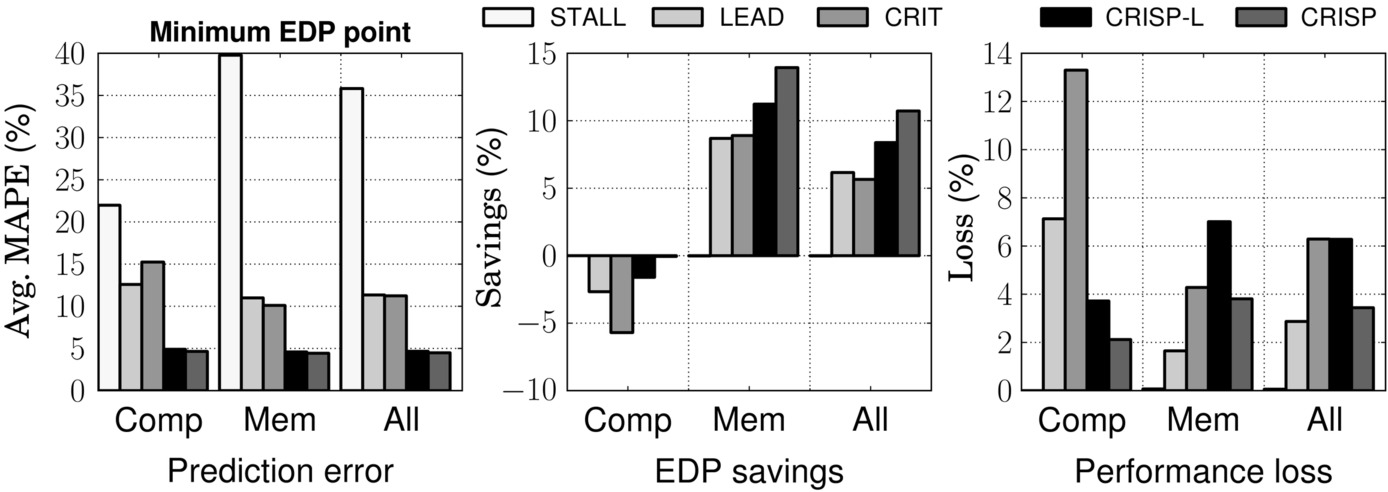
CRISP can be simplified to estimate the LCP length as the total number of load outstanding cycles, without regard for which stall cycles, and in particular, which computation are under the critical path. We simply treat all computation cycles that are overlapped by a load as though they were on the critical path. This approximated version of CRISP (CRISP-L) requires three counters, and thus removes 98% of the storage overhead of CRISP (all the time-stamp registers).
CRISP-L demonstrates competitive prediction accuracy (4.66% on average in Fig. 20) as CRISP (4.48% on average) does for the experiment in Section 5.1. However, when used in an EDP controller, CRISP-L suffers relative to CRISP, but still realizes far better (8.38%) EDP savings than CRIT (5.65%) and LEAD (6.16%). The inclusion of more compute cycles in LCP tends to create underpredictions of execution time, resulting in more aggressive frequency scaling. CRISP-L experiences more (6.28%) performance loss than CRISP (3.44%).
5.4 Generality of CRISP
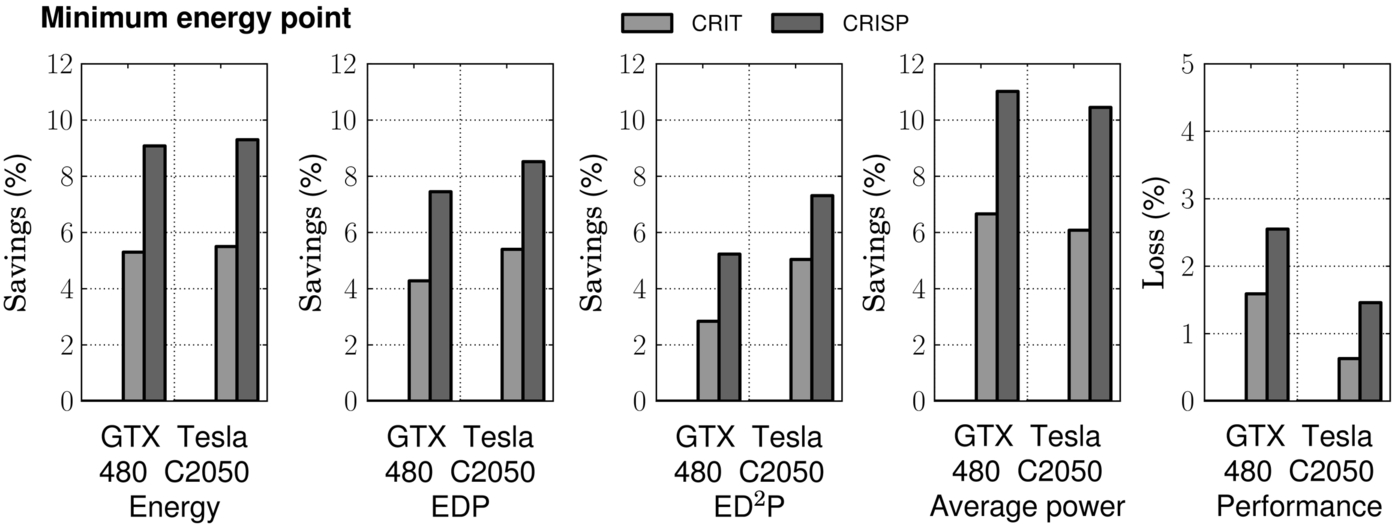
All of the results so far were for a NVIDIA GTX 480 GPU. To demonstrate that the CRISP model is more general, we replicated the same experiments for a modeled Tesla C2050 GPU. The Tesla differs in available clock frequency settings, number of cores, DRAM queue size, and in the topology of the interconnect. Results for predictor accuracy and effectiveness were consistent with the prior results. In this section, we show in particular the result for the EDP-optimized controller. Fig. 21 shows that the mean absolute percentage prediction error of CRISP (6.2%) is much lower than LEAD (16.9%) and CRIT (15.4%). Meanwhile, CRISP realizes 10.3% EDP savings, which is 5% more than the best of the prior models.
We also experimented with another DVFS controller goal; this one seeks to minimize energy while keeping the performance overhead under 1%. Fig. 22 shows the energy, EDP, ED2P, average power savings, and the performance loss for GTX480 and Tesla C2050. In Tesla C2050, CRISP achieves 9.3% energy savings, which is 4% more than CRIT.
6 Conclusion
We introduce the CRISP performance model to enable effective DVFS control in GPGPUs. Existing DVFS models targeting CPUs do not capture key GPGPU execution characteristics, causing them to miss energy savings opportunities or causing unintended performance loss. CRISP effectively handles the impact of highly overlapped memory and computation in a system with high thread-level parallelism, and also captures the effect of frequent memory store-based stalls.