2. Analog Signals

As we stated in the last chapter, the first step in understanding digital signal processing is to learn about analog signals. With that thought in mind, the goal of this chapter is to define and explain the nature of analog signals.

• typically varies in value over time,

• has a value at all instants in time, and

• contains information.

Those characteristics seem a little mysterious but they’re really not. You experience analog signals every day. The audio emanating from your cell phone speaker, the electrical video signal arriving from your television cable company, the height of the mercury column in an outdoor thermometer over a period of one day, and the fluctuating light intensity from a twinkling nighttime star are all examples of analog signals. An important aspect of analog signals is that they contain information that can be meaningful to us. With that said, let’s look at a few analog signals in detail.

Figure 2-1 High and low outdoor temperatures in Marquette, Michigan.

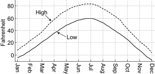
A requirement for analog signals is that when drawn on a piece of paper, with time represented on the horizontal axis as shown in Figure 2-1, the tip of the pen or pencil never leaves the surface of the paper. There are no gaps, no missing information, in the curve. Such a curve can be called a continuous curve. In fact, many engineers refer to analog signals as continuous signals.

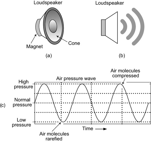
Figure 2-2 Audio tone analog sound wave:(a) loudspeaker; (b) loudspeaker and emanating air pressure waves; (c) tuning-fork wave of fluctuating air pressure entering a human ear as time passes.

When sound coming from a loudspeaker is a single audio tone, like the tone produced by a tuning fork, the fluctuating air pressure waves entering the listener’s ears can be depicted as shown in Figure 2-2(c). When the loudspeaker cone moves outward, it compresses air molecules creating a small region of high air pressure. Then, when the loudspeaker cone moves inward, it creates a small region of low air pressure. Thus, the loudspeaker produces radiating regions of compressed and rarefied air molecules, waves of high and low air pressure that travel from the loudspeaker to the listener’s ears.

Human ears are sensitive to these waves of fluctuating air pressure. When these waves enter our ears, an electrical signal is transmitted to our brains and only then do we experience the sensation of sound.

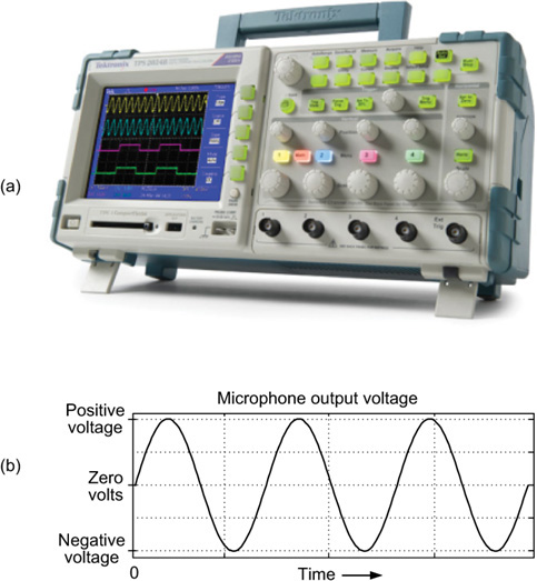
Figure 2-3 Viewing a microphone’s output: (a) a modern oscilloscope (courtesy of Tektronix Inc.); (b) displayed microphone output analog voltage waveform of a tuning-fork sound.

If the tuning-fork sound wave in Figure 2-2(c) arrives at a microphone and the microphone’s output cable is connected to the input port of an oscilloscope, then the scope’s display would show the voltage signal as depicted in Figure 2-3(b). The voltage at any instant in time is called the amplitude of the voltage waveform and indicates its instantaneous energy. The peak positive voltage in Figure 2-3(b) is called the peak amplitude of the waveform. High peak-amplitude waveforms have more energy than low peak-amplitude waveforms.

The microphone’s output voltage, representing fluctuations in air pressure, is an analog signal because it

• has an amplitude that varies as time passes,

• has a value at all instants in time (the voltage value changes smoothly in a continuous curve, with no gaps), and

• contains information such as peak-to-trough voltage difference and frequency (oscillations per second).

Again, the curve in Figure 2-3(b) is a voltage representation of the Figure 2-2(b) sound wave produced by a tuning fork. Thus, we can say that the Figure 2-3(b) voltage signal is analogous to, or the analogue of, the sound wave traveling in air. We referred to the curve in the figure as a fluctuating voltage. Because so many of the real-world analog signals that interest us take the form of analog voltage signals, let’s pause for a moment and consider what is meant by voltage.

Figure 2-4 Voltage across a lightbulb: (a) switch open; (b) switch closed.

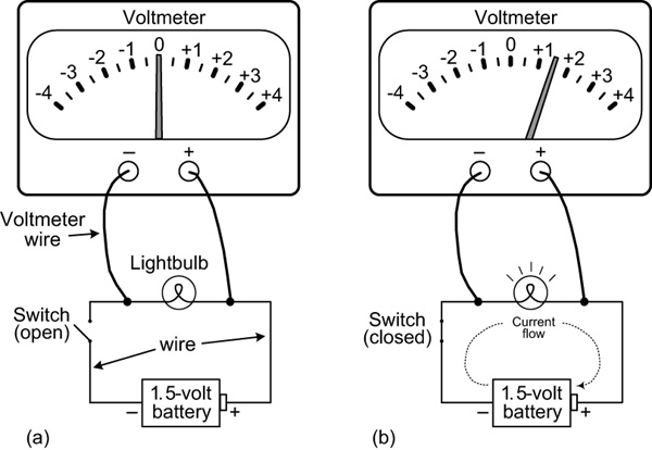
When the switch is closed, as shown in Figure 2-4(b), there is now an electrical path for electron current to flow through the wire clockwise from the negative terminal of the battery to its positive terminal, a +1.5 volt voltage is applied across the lightbulb terminals, and the bulb is lit. Specifically, electron current flows through the lightbulb and the bulb’s filament becomes white hot, emitting visible light.

When the switch is closed, as in in Figure 2-4(b), the +1.5 volt voltage applied to the lightbulb is referred to as a DC voltage. The acronym DC stands for direct current, and for us DC voltage merely means a voltage that remains constant in value as time passes.

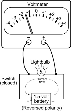
Let’s consider another battery/lightbulb scenario. If we turned Figure 2-4’s battery around, reversing its polarity, and closed the switch, then electron current would flow in a counterclockwise direction as shown in Figure 2-5. In that case, the voltmeter measures a negative –1.5 volts across the bulb’s terminals. (Incandescent lightbulbs generate visible light regardless of the direction of current flow through their filaments.)

Figure 2-5 Voltage applied to a lightbulb with reversed battery polarity and switch closed.

There are two concepts to learn from Figures 2-4 and 2-5. First, voltage is an electrical pressure that, when applied to some hardware component (the lightbulb), does work for us. If the lightbulb in Figure 2-4 were replaced by a low-voltage electric motor, then closing the switch would cause the motor to turn. This is how battery-operated screwdrivers work. Second, voltages have a polarity associated with them, as shown by the voltmeter readings in Figures 2-4(b) and 2-5.

• waves in a river or ocean

• sound waves

• electromagnetic waves radiated by AM and FM broadcast stations

• seismic waves (earthquakes)

• starlight in the night sky

In fact, right now you’re probably no farther than 10 feet from a voltage that fluctuates in a sinusoidal manner. We’re referring to the oscillating voltage at the conductors of your 120 volt AC (alternating current) wall socket. In Europe, it would be a 220 volt AC wall socket.

The voltage waveform in Figure 2-3(b) is a specific kind of sinusoidal wave called a sine wave, and sine waves show up in almost every aspect of digital signal processing. As such, we now take a closer look at sine waves.

1. That would be close to 200 feet above ground level for Big Ben on the Elizabeth Tower, nicknamed for its largest bell.

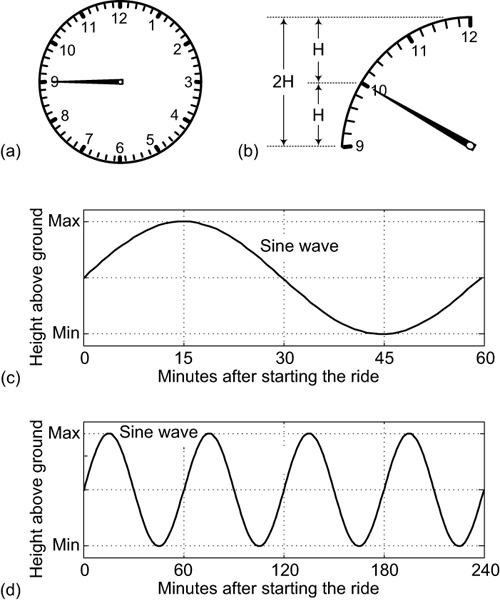
Figure 2-6 Riding Big Ben’s minute hand: (a) starting point; (b) halfway point; (c) height versus one hour of time; (d) height versus four hours of time.

Continuing his ride, our daredevil would be at his original height when the minute hand is horizontal again pointing to 3, and at the minimum height at 6, the bottom of the hour. He would then finish his ride at the 9 position where he started.

If we were to sketch the relative height our young lad achieved during his hour of joy-riding, we would plot a single cycle of the well-known sine wave curve in Figure 2-6(c). This shows the important fundamental relationship between a sine wave and the vertical height of points around the perimeter of a circle. Figure 2-6(d) shows four cycles of a sine wave.

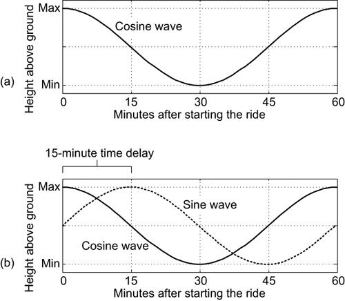
Figure 2-7 Riding Big Ben’s minute hand starting at the 12 position: (a) height versus time; (b) time relationship between a sine wave and a cosine wave.

A sine wave is a delayed-in-time version of a cosine wave. Engineers call this relationship “a phase shift of one-quarter cycle between the sine and cosine,” or in our case, one-quarter hour as depicted in Figure 2-7(b). Both sine waves and cosine waves are known as sinusoidal waves. Believe it or not, you’ve just learned the basics of sines and cosines!

Now here’s how we adjust this knowledge to the world of engineering. The ancients used a circle rather than a clock to describe sines and cosines.² Instead of a clockwise rotating minute hand, they used a line 1 unit in length, representing the radius of a circle that rotates counterclockwise through 360 degrees around a circle, as shown in the two-dimensional Figure 2-8. For us, this unit-length line is represented by the bold arrow in the figure. The zero in the center of the circle represents a point where the x-axis value is zero and the y-axis value is zero.

2. Among the ancients are Babylonians, Sumerians, and Greeks—not your authors.

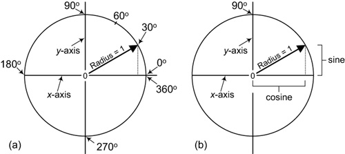
Figure 2-8 (a) Engineering basis for sines and cosines; (b) horizontal and vertical distance representations.

The arrow starts by pointing to the right side at 0 degrees and proceeds counterclockwise around the circle 360 degrees back to where it started. During one arrow rotation, the vertical distance of the arrow tip above or below the x-axis is represented by the sine wave curve in Figure 2-6(c). The horizontal distance of the arrow tip to the right or the left of the y-axis is represented by the cosine wave curve in Figure 2-7(a). Those representations are shown in Figure 2-8(b).

At this point, you might think that we’ve spent too much time here describing sine and cosine waves. To that we say sine and cosine waves pervade every aspect of both analog and digital signal processing, and time spent understanding sine and cosine waves is never wasted time. OK, with that said, let’s explore the topic of voltages once more.

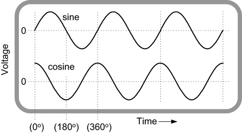
Figure 2-9 Oscilloscope display showing the time relationship between a sine wave voltage and a cosine wave voltage.

Figure 2-10 shows what is called a square wave voltage that repeats its cycle once every half second; that is, two oscillations/second. We say that the period of that square wave is 0.5 seconds, meaning that it repeats its oscillation once every 0.5 seconds. Notice how that bi-level voltage very quickly fluctuates back and forth between two distinct voltage levels. As you can see, a square wave signal is not necessarily square in its shape; the voltage in Figure 2-10 is more rectangular than square. Nevertheless, when you hear someone talk about a square wave, what they actually mean is a signal that toggles between its two voltage levels and spends 50% of its time at each level. (The bottom two voltage waveforms on the oscilloscope in Figure 2-3(a) are square waves.)

Figure 2-10 Analog square wave.

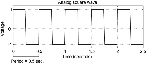
For now, we’ll call Figure 2-10 an analog square wave because it meets one of our most important definitions of an analog signal. Namely, when we draw the square wave signal on a piece of paper, the tip of our pen or pencil never leaves the surface of the paper. The square wave is continuous.

Inside your desktop and laptop computers, there is a square wave voltage called the clock signal. This constant-period square wave voltage is used to synchronize various circuit operations within your computer. When you read that a computer’s clock frequency is 500 megahertz (Mhz), this means the computer generates and uses an internal square wave clock voltage oscillating 500 million times per second. The higher the clock frequency, the faster will be a computer’s operating speed. In technical terms, a frequency of one oscillation per second is referred to as one hertz (Hz). We’ll discuss the notion of frequency in more detail in the next chapter.

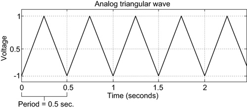
Now and then, you may hear signal processing engineers speak of a triangular wave voltage. This is a periodic voltage waveform as shown in Figure 2-11. It’s easy to see why that signal is called a triangular voltage.

Figure 2-11 Periodic triangular-wave analog signal.

We’ll encounter square and triangular waves again in the next chapter. Now that we’re somewhat comfortable with the meaning of the word voltage, we’ll return to the topic of analog signals.

Figure 2-12 Analog audio speech signal: (a) “Mister Spock”; (b) “Mis.”

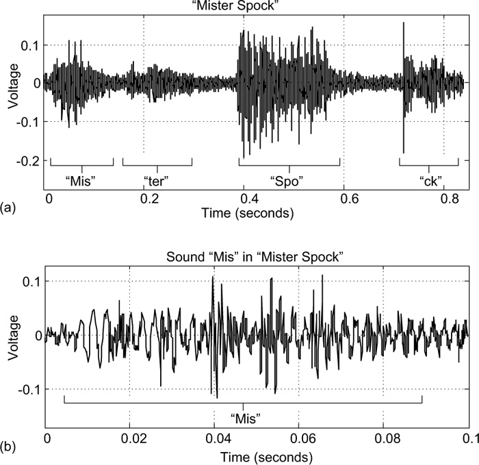
We can examine the complicated pattern of the analog voltage in Figure 2-12(a) further by zooming in on the first syllable of the word “Mister.” Figure 2-12(b) shows the details of the voltage waveform of just the syllable “Mis.” Signal processing people work with voltage waveforms like this every day. They collect, examine, characterize, and sometimes modify these sorts of analog signals. In later chapters, we’ll learn about the useful operations that can be performed on analog signals.

You may think we belabored the subject of analog signals a bit too much in this chapter, especially for a book about digital signal processing. Don’t worry, we’re not wasting time, paper, or ink. All of the concepts we learned about analog signals will help us understand digital signals.

The concepts you should remember from this chapter are:

• Analog signals are information-carrying physical quantities that vary in value as time passes.

• Physical quantities such as speed, vibration, temperature, sound pressure, and light intensity can be converted to voltages on a cable, allowing them to be viewed on the screen of an oscilloscope.

• Signal processing engineers work primarily with analog signals in the form of time-varying voltages.

• Periodically varying voltages, like sine and cosine wave voltages, are very common in the world of signal processing.

• The repetition rate, per unit time, of a periodic voltage is called frequency.

• Frequency is most commonly measured in units of hertz (Hz). One Hz is equal to one cycle per second.