8.1 . (In fact, we always get doubles with probability when at least one of the dice is fair.) Any two faces whose sum is 7 have the same probability in distribution Pr₁, so S = 7 has the same probability as doubles.

8.2 There are 12 ways to specify the top and bottom cards and 50! ways to arrange the others; so the probability is 12.50!/52! = 12/(51.52) = .

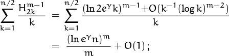
8.3 (3 + 2 + · · · + 9 + 2) = 4.8; (3² + 2² + · · · + 9² + 2² – 10(4.8)²) = , which is approximately 8.6. The true mean and variance with a fair coin are 6 and 22, so Stanford had an unusually heads-up class. The corresponding Princeton figures are 6.4 and . 12.5 (This distribution has κ₄ = 2974, which is rather large. Hence the standard deviation of this variance estimate when n = 10 is also rather large, 20.1 according to exercise 54. One cannot complain that the students cheated.)

8.4 This follows from (8.38) and (8.39), because F(z) = G(z)H(z). (A similar formula holds for all the cumulants, even though F(z) and G(z) may have negative coefficients.)

8.5 Replace H by p and T by q = 1 – p. If S_A = S_B = we have p²qN = and pq²N = q + ; the solution is p = 1/φ², q = 1/φ.

8.6 In this case X|y has the same distribution as X, for all y, hence E(X|Y) = EX is constant and V(E(X|Y)) = 0. Also V(X|Y) is constant and equal to its expected value.

8.7 We have by Chebyshev’s monotonic inequality of Chapter 2.

8.8 Let p = Pr(ω A ∩ B), q = Pr(ω ∉A), and r = Pr(ω ∉B). Then p + q + r = 1, and the identity to be proved is p = (p + r)(p + q) – qr.

8.9 This is true (subject to the obvious proviso that F and G are defined on the respective ranges of X and Y), because

8.10 Two. Let x₁ < x₂ be distinct median elements; then 1 ≤ Pr(X ≤ x₁) + Pr(X ≥ x₂) ≤ 1, hence equality holds. (Some discrete distributions have no median elements. For example, let Ω be the set of all fractions of the form ±1/n, with Pr(+1/n) = Pr(–1/n)= .)

8.11 For example, let K = k with probability 4/(k + 1)(k + 2)(k + 3), for all integers k ≥ 0. Then EK = 1, but E(K²) = ∞. (Similarly we can construct random variables with finite cumulants through κ_m but with κ_m+1 = ∞.)

8.12 (a) Let p_k = Pr(X = k). If 0 < x ≤ 1, we have Pr(X ≤ r) = ∑_k≤rp_k ≤ ∑_k≤r x^k–rp_k ≤ ∑_k x^k–rp_k = x^–rP(x). The other inequality has a similar proof. (b) Let x = α/(1–α) to minimize the right-hand side. (A more precise estimate for the given sum is obtained in exercise 9.42.)

8.13 (Solution by Boris Pittel.) Let us set Y = (X₁ + · · · + X_n)/n and Z = (X_n+1 + · · · + X_2n)/n. Then

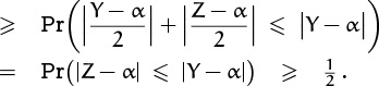
The last inequality is, in fact, ‘>’ in any discrete probability distribution, because Pr(Y = Z) > 0.

8.14 Mean(H) = p Mean(F) + q Mean(G); Var(H) = p Var(F) + q Var(G) + pq (Mean(F)–Mean(G))². (A mixture is actually a special case of conditional probabilities: Let Y be the coin, let X|H be generated by F(z), and let X|T be generated by G(z). Then VX = EV(X|Y) + VE(X|Y), where EV(X|Y) = pV(X|H) + qV(X|T) and VE(X|Y) is the variance of pz^Mean(F)+ qz^Mean(G).)

8.15 By the chain rule, H′(z) = G′(z)F′ (G(z)); H″(z) = G″(z)F′ (G(z)) + G′(z)²F′′ (G(z)). Hence

Mean(H) = Mean(F) Mean(G);

   Var(H) = Var(F) Mean(G)² + Mean(F) Var(G).

(The random variable corresponding to probability distribution H can be understood as follows: Determine a nonnegative integer n by distribution F; then add the values of n independent random variables that have distribution G. The identity for variance in this exercise is a special case of (8.106), when X has distribution H and Y has distribution F.)

8.16 e^w(z–1)/(1 – w).

8.17 Pr(Y_n,p ≤ m) = Pr(Y_n,p + n ≤ m + n) = probability that we need ≤ m + n tosses to obtain n heads = probability that m + n tosses yield ≥ n heads = Pr(X_m+n,p ≥ n). Thus

and this is (5.19) with n = r, x = q, y = p.

8.18 (a) G_X(z) = e^μ(z–1). (b) The mth cumulant is μ, for all m ≥ 1. (The case μ = 1 is called F_∞ in (8.55).)

8.19 (a) G_X1+X2(z) = G_X1(z)G_X2(z) = e^{(μ₁+μ₂)(z–1)}. Hence the probability is e^{–μ₁–μ₂} (μ₁ + μ₂)ⁿ/n!; the sum of independent Poisson variables is Poisson. (b) In general, if K_mX denotes the mth cumulant of a random variable X, we have K_m(aX₁ + bX₂) = a^m(K_mX₁) + b^m(K_mX₂), when a, b ≥ 0. Hence the answer is 2^mμ₁ + 3^mμ₂.

8.20 The general pgf will be G(z) = z^m/F(z), where

8.21 This is ∑_n≥0 q_n, where q_n is the probability that the game between Alice and Bill is still incomplete after n flips. Let p_n be the probability that the game ends at the nth flip; then p_n + q_n = q_n–1. Hence the average time to play the game is ∑_n≥1np_n = (q₀ – q₁) + 2(q₁ – q₂) + 3(q₂ – q₃) + · · · = q₀ + q₁ + q₂ + · · · = N, since lim_n→∞ nq_n = 0.

Another way to establish this answer is to replace H and T by z. Then the derivative of the first equation in (8.78) tells us that .

By the way, .

8.22 By definition we have V(X|Y) = E(X²|Y)–(E(X|Y))²⁾ and V(E(X|Y)) = E((E(X|Y))²)–(E(E(X|Y)))²; hence E(V(X|Y))+ V(E(X|Y))= E(E(X²|Y))–(E(E(X|Y)))². But E(E(X|Y))= ∑_y Pr(Y = y)E(X|y) = ∑_x,y Pr(Y = y) × Pr((X|y) = x)x = EX and E(E(X²|Y)) = E(X²), so the result is just VX.

8.23 Let and ; and let Ω₂ be the other 16 elements of Ω. Then according as ω Ω₀, Ω₁, Ω₂. The events A must therefore be chosen with k_j elements from Ω_j, where (k₀, k₁, k₂) is one of the following: (0, 0, 0), (0, 2, 7), (0, 4, 14), (1, 4, 4), (1, 6, 11), (2, 6, 1), (2, 8, 8), (2, 10, 15), (3, 10, 5), (3, 12, 12), (4, 12, 2), (4, 14, 9), (4, 16, 16). For example, there are events of type (2, 6, 1). The total number of such events is [z⁰](1 + z²⁰)⁴(1 + z^–7)¹⁶(1 + z²)¹⁶, which turns out to be 1304872090. If we restrict ourselves to events that depend on S only, we get 40 solutions S A, where , and the complements of these sets. (Here the notation ‘’ means either 2 or 12 but not both.)

8.24 (a) Any one of the dice ends up in J’s possession with probability ; hence . Let . Then the pgf for J’s total holdings is (q + pz)²ⁿ⁺¹, with mean (2n + 1)p and variance (2n + 1)pq, by (8.61). (b) .

8.25 The pgf for the current stake after n rolls is G_n(z), where

(The noninteger exponents cause no trouble.) It follows that Mean(G_n) = Mean(G_n–1), and . So the mean is always A, but the variance grows to .

This problem can perhaps be solved more easily without generating functions than with them.

8.26 The pgf F_l,n(z) satisfies ; hence and ; the variance is easily computed. (In fact, we have

which approaches a Poisson distribution with mean 1/l as n → ∞.)

8.27 (n²Σ₃ – 3nΣ₂Σ₁ + 2Σ)/n(n – 1)(n – 2) has the desired mean, where . This follows from the identities

EΣ3 =	nμ3;
E(Σ2Σ1) =	nμ3 + n(n – 1)μ2μ1;
E(Σ) =	nμ3 + 3n(n – 1)μ2μ1 + n(n – 1)(n – 2)μ.

Incidentally, the third cumulant is κ₃ = E((X–EX)³), but the fourth cumulant does not have such a simple expression; we have κ₄ = E((X – EX)⁴)– 3(VX)².

8.28 (The exercise implicitly calls for p = q =, but the general answer is given here for completeness.) Replace H by pz and T by qz, getting S_A(z) = p²qz³/(1 – pz)(1 – qz)(1 – pqz²) and S_B(z) = pq²z³/(1 – qz)(1 – pqz²). The pgf for the conditional probability that Alice wins at the nth flip, given that she wins the game, is

This is a product of pseudo-pgf’s, whose mean is 3+p/q+q/p+2pq/(1–pq). The formulas for Bill are the same but without the factor q/(1 – pz), so Bill’s mean is 3 + q/p + 2pq/(1 – pq). When p = q =, the answer in case (a) is ; in case (b) it is . Bill wins only half as often, but when he does win he tends to win sooner. The overall average number of flips is , agreeing with exercise 21. The solitaire game for each pattern has a waiting time of 8.

8.29 Set H = T = in

1 + N(H + T) = N + S_A + S_B + S_C

 N HHTH = S_A(HTH + 1) + S_B(HTH + TH) + S_C(HTH + TH)

 N HTHH = S_A(THH + H) + S_B(THH + 1) + S_C(THH)

 N THHH = S_A(HH) + S_B(H) + S_C

to get the winning probabilities. In general we will have S_A + S_B + S_C = 1 and

S_A(A:A) + S_B(B:A) + S_C(C:A) = S_A(A:B) + S_B(B:B) + S_C(C:B)

      = S_A(A:C) + S_B(B:C) + S_C(C:C).

In particular, the equations 9S_A + 3S_B + 3S_C = 5S_A + 9S_B + S_C = 2S_A + 4S_B + 8S_C imply that , , .

8.30 The variance of P(h₁, . . . , h_n; k)|k is the variance of the shifted binomial distribution ((m – 1 + z)/m)^k–1z, which is by (8.61). Hence the average of the variance is Mean(S)(m – 1)/m². The variance of the average is the variance of (k – 1)/m, namely Var(S)/m². According to (8.106), the sum of these two quantities should be VP, and it is. Indeed, we have just replayed the derivation of (8.96) in slight disguise. (See exercise 15.)

8.31 (a) A brute force solution would set up five equations in five unknowns:

A = 1;   B = zA + zC;   C = zB + zD;

D = zC + zE;   E = zD + zA.

But positions C and D are equidistant from the goal, as are B and E, so we can set C = D and B = E in these generating functions for the probabilities. Only two equations now remain to be solved:

B = z + zC;   C = zB + zC.

Hence C = z²/(4 – 2z – z²); we have Mean(C) = 6 and Var(C) = 22. (Rings a bell? In fact, this problem is equivalent to flipping a fair coin until getting heads twice in a row: Heads means “advance toward the apple” and tails means “start over.”) (b) Chebyshev’s inequality says that Pr(C ≥ 100) = Pr((C – 6)² ≥ 94²) ≤ 22/94² ≈ .0025. (c) The second tail inequality says that Pr(C ≥ 100) ≤ 1/(x⁹⁸(4 – 2x – x²)) for all x ≥ 1, and we get the upper bound 0.00000005 when . (The actual probability is ∑_n≥100 F_n–1/2ⁿ = F₁₀₁/2⁹⁹ ≈ 0.0000000009, according to exercise 37.)

8.32 By symmetry, we can reduce each month’s situation to one of four possibilities:

D, the states are diagonally opposite;

A, the states are adjacent and not Kansas;

K, the states are Kansas and one other;

S, the states are the same.

“Toto, I’ve a feeling we’re not in Kansas anymore.”

—Dorothy

Considering the Markovian transitions, we get four equations

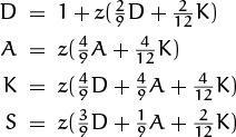
whose sum is D + K + A + S = 1 + z(D + A + K). The solution is

but the simplest way to find the mean and variance may be to write z = 1+w and expand in powers of w, ignoring multiples of w²:

Now , and . The mean is and the variance is . (Is there a simpler way?)

8.33 First answer: Clearly yes, because the hash values h₁, . . . , h_n are independent. Second answer: Certainly no, even though the hash values h₁, . . . , h_n are independent. We have Pr(X_j = 0) = s_k [j ≠ k](m–1)/m = (1 – s_j)(m – 1)/m, but Pr(X₁ = X₂ = 0) = s_k[k > 2](m – 1)²/m² = (1 – s₁ – s₂)(m – 1)²/m² ≠ Pr(X₁ = 0) Pr(X₂ = 0).

8.34 Let [zⁿ] S_m(z) be the probability that Gina has advanced < m steps after taking n turns. Then S_m(1) is her average score on a par-m hole; [z^m] S_m(z) is the probability that she loses such a hole against a steady player; and 1 – [z^m–1] S_m(z) is the probability that she wins it. We have the recurrence

 S₀(z) = 0;

S_m(z) = 1 + pzS_m–2(z) + qzS_m–1(z)/(1 – rz),   for m > 0.

To solve part (a), it suffices to compute the coefficients for m, n ≤ 4; it is convenient to replace z by 100w so that the computations involve nothing but integers. We obtain the following tableau of coefficients:

S0	0	0	0	0	0
S1	1	4	16	64	256
S2	1	95	744	4432	23552
S3	1	100	9065	104044	819808
S4	1	100	9975	868535	12964304

Therefore Gina wins with probability 1 – .868535 = .131465; she loses with probability .12964304. (b) To find the mean number of strokes, we compute

(Incidentally, S₅(1) ≈ 4.9995; she wins with respect to both holes and strokes on a par-5 hole, but loses either way when par is 3.)

8.35 The condition will be true for all n if and only if it is true for n = 1, by the Chinese remainder theorem. One necessary and sufficient condition is the polynomial identity

(p₂+p₄+p₆ + (p₁+p₃+p₅)w)(p₃+p₆ + (p₁+p₄)z + (p₂+p₅)z²) = (p₁wz + p₂z² + p₃w + p₄z + p₅wz² + p₆),

but that just more-or-less restates the problem. A simpler characterization is

(p2 + p4 + p6)(p3 + p6) = p6,

(p1 + p3 + p5)(p2 + p5) = p5,

which checks only two of the coefficients in the former product. The general solution has three degrees of freedom: Let a₀ + a₁ = b₀ + b₁ + b₂ = 1, and put p₁ = a₁b₁, p₂ = a₀b₂, p₃ = a₁b₀, p₄ = a₀b₁, p₅ = a₁b₂, p₆ = a₀b₀.

8.36 (a) (b) If the kth die has faces with s₁, . . . , s₆ spots, let p_k(z) = z^s₁ + · · · + z^s₆. We want to find such polynomials with p₁(z) . . . p_n(z) = (z + z² + z³ + z⁴ + z⁵ + z⁶)ⁿ. The irreducible factors of this polynomial with rational coefficients are zⁿ(z + 1)ⁿ × (z² + z + 1)ⁿ(z² – z + 1)ⁿ; hence p_k(z) must be of the form z^a_k (z + 1)^b_k × (z² + z + 1)^c_k (z² – z + 1)^d_k. We must have a_k ≥ 1, since p_k(0) = 0; and in fact a_k = 1, since a₁ + · · · + a_n = n. Furthermore the condition p_k(1) = 6 implies that b_k = c_k = 1. It is now easy to see that 0 ≤ d_k ≤ 2, since d_k > 2 gives negative coefficients. When d = 0 and d = 2, we get the two dice in part (a); therefore the only solutions have k pairs of dice as in (a), plus n – 2k ordinary dice, for some .

8.37 The number of coin-toss sequences of length n is F_n–1, for all n > 0, because of the relation between domino tilings and coin flips. Therefore the probability that exactly n tosses are needed is F_n–1/2ⁿ, when the coin is fair. Also q_n = F_n+1/2^n–1, since ∑_k≥n F_kz^k = (F_nzⁿ + F_n–1zⁿ⁺¹)/(1 – z – z²). (A systematic solution via generating functions is, of course, also possible.)

8.38 When k faces have been seen, the task of rolling a new one is equivalent to flipping coins with success probability p_k = (m – k)/m. Hence the pgf is . The mean is ; the variance is ; and equation (7.47) provides a closed form for the requested probability, namely . (The problem discussed in this exercise is traditionally called “coupon collecting.”)

8.39 E(X) = P(–1); V(X) = P(–2) – P(–1)²; E(ln X) = –P′(0).

8.40 (a) We have , by (7.49). Incidentally, the third cumulant is npq(q–p) and the fourth is npq(1–6pq). The identity q+pe^t = (p+qe^–t)e^t shows that f_m(p) = (–1)^mf_m(q)+[m = 1]; hence we can write f_m(p) = g_m(pq)(q – p)^{[m odd]}, where g_m is a polynomial of degree m/2, whenever m > 1. (b) Let p = and F(t) = ln( + e^t). Then ∑_m≥1 κ_mt^{m –1}/(m–1)! = F′(t) = 1–1/(e^t+1), and we can use exercise 6.23.

8.41 If G(z) is the pgf for a random variable X that assumes only positive integer values, then G(z) dz/z = Pk–1 Pr(X = k)/k = E(X^–1). If X is the distribution of the number of flips to obtain n + 1 heads, we have G(z) = (pz/(1 – qz))ⁿ⁺¹ by (8.59), and the integral is

if we substitute w = pz/(1 – qz). When p = q the integrand can be written (–1)ⁿ((1+w)^–1–1+w–w²+· · ·+(–1)ⁿw^n–1), so the integral is . We have by (9.28), and it follows that .

8.42 Let F_n(z) and G_n(z) be pgf’s for the number of employed evenings, if the man is initially unemployed or employed, respectively. Let q_h = 1 – p_h and q_f = 1 – p_f. Then F₀(z) = G₀(z) = 1, and

F_n(z) = p_hzG_n–1(z) + q_hF_n–1(z);

G_n(z) = p_fF_n–1(z) + q_fzG_n–1(z).

The solution is given by the super generating function

where B(w) = w(q_f –(q_f –p_h)w)/(1–q_hw) and A(w) =(1–B(w))/(1–w).

Now ∑_n≥0(1)wⁿ = αw/(1 – w)² + β/(1 – w) – β/1 – (q_f – p_h)w) where

hence (1) = αn + β(1 – (q_f – p_h)ⁿ). (Similarly (1) = α²n² + O(n), so the variance is O(n).)

8.43 G_n(z) = ∑_k≥0 z^k/n! = z/n!, by (6.11). This is a product of binomial pgf’s, , where the kth has mean 1/k and variance (k – 1)/k²; hence Mean(G_n) = H_n and Var (G_n) = H_n – .

8.44 (a) The champion must be undefeated in n rounds, so the answer is pⁿ. (b,c) Players x₁, . . . , x_2^k must be “seeded” (by chance) in distinct subtournaments and they must win all 2^k(n – k) of their matches. The 2ⁿ leaves of the tournament tree can be filled in 2ⁿ! ways; to seed it we have 2^k!(2^n–k)^2k ways to place the top 2^k players, and (2ⁿ – 2^k)! ways to place the others. Hence the probability is (2p)^2k(n–k)/. When k = 1 this simplifies to (2p²)^n–1/(2ⁿ – 1). (d) Each tournament outcome corresponds to a permutation of the players: Let y₁ be the champ; let y₂ be the other finalist; let y₃ and y₄ be the players who lost to y₁ and y₂ in the semifinals; let (y₅, . . . , y₈) be those who lost respectively to (y₁, . . . , y₄) in the quarterfinals; etc. (Another proof shows that the first round has 2ⁿ!/2^n–1! essentially different outcomes; the second round has 2^n–1!/2^n–2!; and so on.) (e) Let S_k be the set of 2^k–1 potential opponents of x₂ in the kth round. The conditional probability that x₂ wins, given that x₁ belongs to S_k, is

Pr(x₁ plays x₂)·p^n–1(1 – p) + Pr(x₁ doesn’t play x₂)·pⁿ

                   = p^k–1p^n–1(1 – p) + (1 – p^k–1)pⁿ.

The chance that x₁ S_k is 2^k–1/(2ⁿ – 1); summing on k gives the answer:

(f) Each of the 2ⁿ! tournament outcomes has a certain probability of occurring, and the probability that x_j wins is the sum of these probabilities over all (2ⁿ – 1)! tournament outcomes in which x_j is champion. Consider interchanging x_j with x_j+1 in all those outcomes; this change doesn’t affect the probability if x_j and x_j+1 never meet, but it multiplies the probability by (1 – p)/p < 1 if they do meet.

8.45 (a) A(z) = 1/(3 – 2z); B(z) = zA(z)²; C(z) = z²A(z)³. The pgf for sherry when it’s bottled is z³A(z)³, which is z³ times a negative binomial distribution with parameters n = 3, p = . (b) Mean(A) = 2, Var(A) = 6; Mean(B) = 5, Var(B) = 2 Var(A) = 12; Mean(C) = 8, Var(C) = 18. The sherry is nine years old, on the average. The fraction that’s 25 years old is . (c) Let the coefficient of wⁿ be the pgf for the beginning of year n. Then

Differentiate with respect to z and set z = 1; this makes

The average age of bottled sherry n years after the process started is 1 greater than the coefficient of w^n–1, namely 9–()ⁿ(3n²+21n+72)/8. (This already exceeds 8 when n = 11.)

8.46 (a) P(w, z) = 1 + (wP(w, z) + zP(w, z)) = (1 – (w + z))^–1, hence p_m,n = 2^–m–n. (b) P_k(w, z) = (w^k + z^k)P(w, z); hence

(c) ; this can be summed using (5.20):

(The methods of Chapter 9 show that this is – 1 + O(n^–1/2).

8.47 After n irradiations there are n + 2 equally likely receptors. Let the random variable X_n denote the number of diphages present; then X_n+1 = X_n + Y_n, where Y_n = –1 if the (n + 1)st particle hits a diphage receptor (conditional probability 2X_n/(n + 2)) and Y_n = +2 otherwise. Hence

EX_n+1 = EX_n + EY_n = EX_n – 2EX_n/(n+2) + 2(1 – 2EX_n/(n+2)).

The recurrence (n+2)EX_n+1 = (n–4)EX_n+2n+4 can be solved if we multiply both sides by the summation factor (n + 1)⁵; or we can guess the answer and prove it by induction: EX_n = (2n + 4)/7 for all n > 4. (Incidentally, there are always two diphages and one triphage after five steps, regardless of the configuration after four.)

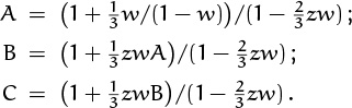
8.48 (a) The distance between frisbees (measured so as to make it an even number) is either 0, 2, or 4 units, initially 4. The corresponding generating functions A, B, C (where, say, [zⁿ] C is the probability of distance 4 after n throws) satisfy

A = zB,   B = zB + zC,   C = 1 + zB + zC.

It follows that A = z²/(16 – 20z + 5z²) = z²/F(z), and we have Mean(A) = 2 – Mean(F) = 12, Var(A) = – Var(F) = 100. (A more difficult but more amusing solution factors A as follows:

where , and p₁ + q₁ = p₂ + q₂ = 1. Thus, the game is equivalent to having two biased coins whose heads probabilities are p₁ and p₂; flip the coins one at a time until they have both come up heads, and the total number of flips will have the same distribution as the number of frisbee throws. The mean and variance of the waiting times for these two coins are respectively and , hence the total mean and variance are 12 and 100 as before.)

(b) Expanding the generating function in partial fractions makes it possible to sum the probabilities. (Note that /(4ϕ) + ϕ²/4 = 1, so the answer can be stated in terms of powers of φ.) The game will last more than n steps with probability 5^(n–1)/24^–n(φⁿ⁺² – φ^–n–2); when n is even this is 5^n/24^–nF_n+2. So the answer is 5⁵⁰4^–100F₁₀₂ ≈ .00006.

8.49 (a) If n > 0, P_N(0, n) = [N = 0] + P_N–1(0, n) + P_N–1(1, n–1); P_N(m, 0) is similar; P_N(0, 0) = [N = 0]. Hence

g_m,n = zg_m–1,n+1 + zg_m,n + zg_m+1,n–1;

 g_0,n = + zg_0,n + g_1,n–1;   etc.

(b) ; ; etc. By induction on m, we have for all m, n ≥ 0. And since , we must have . (c) The recurrence is satisfied when mn > 0, because

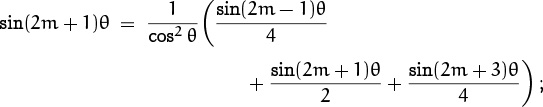
this is a consequence of the identity sin(x – y) + sin(x + y) = 2 sin x cos y. So all that remains is to check the boundary conditions.

8.50 (a) Using the hint, we get

now look at the coefficient of z^3+l. (b) . (c) Let . One can show that (z–3+r)(z–3–r) = 4z, and hence that (r/(1 – z) + 2)² = (13 – 5z + 4r)/(1 – z) = (9 – H(z))/(1 – H(z)).

(d) Evaluating the first derivative at z = 1 shows that Mean(H) = 1. The second derivative diverges at z = 1, so the variance is infinite.

8.51 (a) Let H_n(z) be the pgf for your holdings after n rounds of play, with H₀(z) = z. The distribution for n rounds is

H_n+1(z) = H_n(H(z)),

so the result is true by induction (using the amazing identity of the preceding problem). (b) g_n = H_n(0) – H_n–1(0) = 4/n(n + 1)(n + 2) = 4(n – 1)^–3. The mean is 2, and the variance is infinite. (c) The expected number of tickets you buy on the nth round is Mean(H_n) = 1, by exercise 15. So the total expected number of tickets is infinite. (Thus, you almost surely lose eventually, and you expect to lose after the second game, yet you also expect to buy an infinite number of tickets.) (d) Now the pgf after n games is H_n(z)², and the method of part (b) yields a mean of 16 – π² ≈ 2.8. (The sum ∑_k≥11/k² = π²/6 shows up here.)

8.52 If ω and ω′ are events with Pr(ω) > Pr(ω′), then a sequence of n independent experiments will encounter ω more often than ω′, with high probability, because ω will occur very nearly n Pr(ω) times. Consequently, as n → ∞, the probability approaches 1 that the median or mode of the values of X in a sequence of independent trials will be a median or mode of the random variable X.

8.53 We can disprove the statement, even in the special case that each variable is 0 or 1. Let p₀ = Pr(X = Y = Z = 0),  , , where . Then p₀ + p₁ + · · · + p₇ = 1, and the variables are independent in pairs if and only if we have

(p₄ + p₅ + p₆ + p₇)(p₂ + p₃ + p₆ + p₇) = p₆ + p₇,

(p₄ + p₅ + p₆ + p₇)(p₁ + p₃ + p₅ + p₇) = p₅ + p₇,

(p₂ + p₃ + p₆ + p₇)(p₁ + p₃ + p₅ + p₇) = p₃ + p₇.

But Pr(X + Y = Z = 0) ≠ Pr(X + Y = 0) Pr(Z = 0)    p₀ ≠ (p₀ + p₁)(p₀ + p₂ + p₄ + p₆). One solution is

p₀ = p₃ = p₅ = p₆ = 1/4;      p₁ = p₂ = p₄ = p₇ = 0.

This is equivalent to flipping two fair coins and letting X = (the first coin is heads), Y = (the second coin is heads), Z = (the coins differ). Another example, with all probabilities nonzero, is

p₀ = 4/64, p₁ = p₂ = p₄ = 5/64,

p₃ = p₅ = p₆ = 10/64, p₇ = 15/64.

For this reason we say that n variables X₁, . . . , X_n are independent if

Pr(X₁ = x₁ and · · · and X_n = x_n) = Pr(X₁ = x₁) . . . Pr(X_n = x_n);

pairwise independence isn’t enough to guarantee this.

8.54 (See exercise 27 for notation.) We have

     E(Σ) = nμ₄ + n(n–1)μ;

   E(Σ₂Σ) = nμ₄ + 2n(n–1)μ₃μ₁ + n(n–1)μ + n(n–1)(n–2)μ₂μ;

     E(Σ) = nμ₄ + 4n(n–1)μ₃μ₁ + 3n(n–1)μ

              + 6n(n–1)(n–2)μ₂μ + n(n–1)(n–2)(n–3)μ;

it follows that V(X) = κ₄/n + 2κ/(n – 1).

8.55 There are permutations with X = Y, and permutations with X ≠ Y. After the stated procedure, each permutation with X = Y occurs with probability , because we return to step S1 with probability . Similarly, each permutation with X ≠ Y occurs with probability . Choosing p = makes Pr(X = x and Y = y) = for all x and y. (We could therefore make two flips of a fair coin and go back to S1 if both come up heads.)

8.56 If m is even, the frisbees always stay an odd distance apart and the game lasts forever. If m = 2l + 1, the relevant generating functions are

Gm	=	zA1;
A1	=	zA1 + zA2,
Ak	=	zAk–1 + zAk + zAk+1,	for 1 < k < l,
Al	=	zAl–1 + 34 zAl + 1.

(The coefficient [zⁿ] A_k is the probability that the distance between frisbees is 2k after n throws.) Taking a clue from the similar equations in exercise 49, we set z = 1/cos² θ and A₁ = X sin 2θ, where X is to be determined. It follows by induction (not using the equation for A_l) that A_k = X sin 2kθ. Therefore we want to choose X such that

It turns out that X = 2 cos² θ/sin θ cos(2l + 1)θ, hence

The denominator vanishes when θ is an odd multiple of π/(2m); thus 1–q_kz is a root of the denominator for 1 ≤ k ≤ l, and the stated product representation must hold. To find the mean and variance we can write

Trigonometry wins again. Is there a connection with pitching pennies along the angles of the m-gon?

because tan² θ = z – 1 and tan θ = θ + θ³ + · · ·. So we have Mean(G_m) = (m² –1) and Var(G_m) = m²(m² –1). (Note that this implies the identities

The third cumulant of this distribution is m² (m²–1) (4m² – 1); but the pattern of nice cumulant factorizations stops there. There’s a much simpler way to derive the mean: We have G_m + A₁ + · · · + A_l = z(A₁ + · · · + A_l) + 1, hence when z = 1 we have . Since G_m = 1 when z = 1, an easy induction shows that A_k = 4k.)

8.57 We have A:A ≥ 2^l–1 and B:B < 2^l–1 + 2^l–3 and B:A ≥ 2^l–2, hence B:B – B:A ≥ A:A – A:B is possible only if A:B > 2^l–3. This means that , τ₁ = τ₄, τ₂ = τ₅, . . . , τ_l–3 = τ_l. But then A:A ≈ 2^l–1 + 2^l–4 + · · ·, A:B ≈ 2^l–3 +2^l–6 +· · ·, B:A ≈ 2^l–2 +2^l–5 +· · ·, and B:B ≈ 2^l–1 +2^l–4 +· · ·; hence B:B – B:A is less than A:A – A:B after all. (Sharper results have been obtained by Guibas and Odlyzko [168], who show that Bill’s chances are always maximized with one of the two patterns Hτ₁ . . . τ_l–1 or Tτ₁ . . . τ_l–1. Bill’s winning strategy is, in fact, unique; see the following exercise.)

8.58 (Solution by J. Csirik.) If A is H^l or T^l, one of the two sequences matches A and cannot be used. Otherwise let  = τ₁ . . . τ_l–1, H = HÂ, and T = T Â. It is not difficult to verify that H:A = T:A = Â:Â, H:H + T:T = 2^l–1 + 2( Â:Â) + 1, and A:H + A:T = 1 + 2(A:A) – 2^l. Therefore the equation

implies that both fractions equal

Then we can rearrange the original fractions to show that

where pq > 0 and p + q = gcd(2^l–1 + 1, 2^l – 1) = gcd(3, 2^l – 1); so we may assume that l is even and that p = 1, q = 2. It follows that A:A – A:H = (2^l – 1)/3 and A:A–A:T = (2^l+1–2)/3, hence A:H–A:T = (2^l – 1)/3 ≥ 2^l–2. We have A:H ≥ 2^l–2 if and only if A = (TH)^l/2. But then H:H – H:A = A:A – A:H, so 2^l–1 + 1 = 2^l – 1 and l = 2.

(Csirik [69] goes on to show that, when l ≥ 4, Alice can do no better than to play HT^l–3H². But even with this strategy, Bill wins with probability nearly .)

8.59 According to (8.82), we want B:B – B:A > A:A – A:B. One solution is A = TTHH, B = HHH.

8.60 (a) Two cases arise depending on whether h_k ≠ h_n or h_k = h_n:

(b) We can either argue algebraically, taking partial derivatives of G(w, z) with respect to w and z and setting w = z = 1; or we can argue combinatorially: Whatever the values of h₁, . . . , h_n–1, the expected value of P(h₁, . . . , h_n–1, h_n; n) is the same (averaged over h_n), because the hash sequence (h₁, . . . , h_n–1) determines a sequence of list sizes (n₁, n₂, . . . , n_m) such that the stated expected value is ((n₁+1)+(n₂+1)+· · ·+(n_m+1) /m (n – 1 + m)/m. Therefore the random variable EP(h₁, . . . , h_n; n) is independent of (h₁, . . . , h_n–1), hence independent of P(h₁, . . . , h_n; k).

8.61 If 1 ≤ k < l ≤ n, the previous exercise shows that the coefficient of s_ks_l in the variance of the average is zero. Therefore we need only consider the coefficient of , which is

the variance of ((m – 1 + z)/m)^k–1z; and this is (k – 1)(m – 1)/m² as in exercise 30.

8.62 The pgf D_n(z) satisfies the recurrence

We can now derive the recurrence

which has the solution (n+2) (26n + 15) for all n ≥ 11 (regardless of initial conditions). Hence the variance comes to (n + 2) for n ≥ 11.

8.63 (Another question asks if a given sequence of purported cumulants comes from any distribution whatever; for example, κ₂ must be nonnegative, and must be at least , etc. A necessary and sufficient condition for this other problem was found by Hamburger [6], [175].)

9.1 True if the functions are all positive. But otherwise we might have, say, f₁(n) = n³ + n², f₂(n) = –n³, g₁(n) = n⁴ + n, g₂(n) = –n⁴.

9.2 (a) We have n^lnn ≺ cⁿ ≺ (ln n)ⁿ, since (ln n)² ≺ n ln c ≺ n ln ln n.

(b) n^lnlnlnn ≺ (ln n)! ≺ n^lnlnn. (c) Take logarithms to show that (n!)! wins. (d) ; H_Fn ∼ n ln φ wins because φ² = φ + 1 < e.

9.3 Replacing kn by O(n) requires a different C for each k; but each O stands for a single C. In fact, the context of this O requires it to stand for a set of functions of two variables k and n. It would be correct to write .

9.4 For example, lim_n→∞ O(1/n) = 0. On the left, O(1/n) is the set of all functions f(n) such that there are constants C and n₀ with |f(n)| ≤ C/n for all n ≥ n₀. The limit of all functions in that set is 0, so the left-hand side is the singleton set {0}. On the right, there are no variables; 0 represents {0}, the (singleton) set of all “functions of no variables, whose value is zero.” (Can you see the inherent logic here? If not, come back to it next year; you probably can still manipulate O-notation even if you can’t shape your intuitions into rigorous formalisms.)

9.5 Let f(n) = n² and g(n) = 1; then n is in the left set but not in the right, so the statement is false.

9.6 nln + γn + O(lnn).

9.7 (1 – e^–1/n)^–1 = nB₀ – B₁ + B₂n^–1/2! + · · · = n + + O(n^–1).

9.8 For example, let f(n) = n/2!² + n, g(n) = (n/2 – 1) ! n/2! + n. These functions, incidentally, satisfy f(n) = O (ng(n)) and g(n) = O) nf(n)); more extreme examples are clearly possible.

9.9 (For completeness, we assume that there is a side condition n → ∞, so that two constants are implied by each O.) Every function on the left has the form a(n) + b(n), where there exist constants m₀, B, n₀, C such that |a(n) |≤ B |f(n) |for n ≥ m₀ and |b(n) |≤ C |g(n) |for n ≥ n₀. Therefore the left-hand function is at most max(B, C) (|f(n)| +| g(n)|), for n ≥ max(m₀, n₀), so it is a member of the right side.

9.10 If g(x) belongs to the left, so that g(x) = cos y for some y, where |y| ≤ C|x| for some C, then 0 ≤ 1 – g(x) = 2 sin²(y/2) ≤ y² ≤ C²x²; hence the set on the left is contained in the set on the right, and the formula is true.

9.11 The proposition is true. For if, say, |x| ≤ |y|, we have (x + y)² ≤ 4y². Thus (x + y)² = O(x²) + O(y²). Thus O(x + y)² = O ((x + y)²) = O(O(x²) + O(y²)) = O(O(x²)) + O(O(y²)) = O(x²) + O(y²).

9.12 1 + 2/n + O(n^–2) = (1 + 2/n) (1 + O(n^–2)/(1 + 2/n)) by (9.26), and 1/(1 + 2/n) = O(1); now use (9.26).

9.13 nⁿ(1 + 2n^–1 + O(n^–2))ⁿ = nⁿ exp (n(2n^–1 + O(n^–2))) = e²nⁿ + O(n^n–1).

9.14 It is n^n+β exp ((n + β) (α/n – α²/n² + O(n^–3))).

(It’s interesting to compare this formula with the corresponding result for the middle binomial coefficient, exercise 9.60.)

9.15 , so the answer is

9.16 If l is any integer in the range a ≤ l < b we have

Since l + x ≥ l + 1 – x when , this integral is positive when f(x) is nondecreasing.

9.17

9.18 The text’s derivation for the case α = 1 generalizes to give

the answer is 2^2nα(πn)^(1–α)/2α^–1/2(1 + O(n^–1/2+3)).

9.19 H₁₀ = 2.928968254 ≈ 2.928968256; 10! = 3628800 ≈ 3628712.4; B₁₀ = 0.075757576 ≈ 0.075757494; π(10) = 4 ≈ 10.0017845; e^0.1 = 1.10517092 ≈ 1.10517083; ln 1.1 = 0.0953102 ≈ 0.0953083; 1.1111111 . . . ≈ 1.1111; 1.1^0.1 = 1.00957658 ≈ 1.00957643. (The approximation to π(n) gives more significant figures when n is larger; for example, π(10⁹) = 50847534 ≈ 50840742.)

9.20 (a) Yes; the left side is o(n) while the right side is equivalent to O(n). (b) Yes; the left side is e · e^O(1/n). (c) No; the left side is about times the bound on the right.

9.21 We have P_n = p = n (ln p – 1 – 1/ln p + O(1/log n)²), where

It follows that

(A slightly better approximation replaces this O(1/log n)² by the quantity –5.5/(ln n)² + O(log log n/log n)³; then we estimate P_1000000 ≈ 15480992.8.)

What does a drowning analytic number theorist say?

log log log log . . .

9.22 Replace O(n^–2k) by – n^–2k + O(n^–4k) in the expansion of H_nk ; this replaces O(∑₃(n²)) by in (9.53). We have

hence the term O(n^–2) in (9.54) can be replaced by – n^–2 + O(n^–3).

9.23 nh_n = ∑_0≤k<n h_k/(n–k)+2cH_n/(n+1)(n+2). Choose c = e^π2/6 = ∑_k≥0 g_k so that ∑_k≥0 h_k = 0 and h_n = O(log n)/n³. The expansion of ∑_0≤k<n h_k/(n – k) as in (9.60) now yields nh_n = 2cH_n/(n + 1)(n + 2) + O(n^–2), hence

9.24 (a) If ∑_k≥0|f(k)| < ∞ and if f(n – k) = O(f(n)) when 0 ≤ k ≤ n/2, we have

which is 2O(f(n) ∑_k≥0|f(k)|), so this case is proved. (b) But in this case if a_n = b_n = α^–n, the convolution (n + 1)α^–n is not O(α^–n).

9.25 . We may restrict the range of summation to 0 ≤ k ≤ (log n)², say. In this range and , so the summand is

Hence the sum over k is 2–4/n + O(1/n²). Stirling’s approximation can now be applied to , proving (9.2).

9.26 The minimum occurs at a term B_2m/(2m)(2m–1)n^2m–1 where 2m ≈ 2πn+ , and this term is approximately equal to . The absolute error in ln n! is therefore too large to determine n! exactly by rounding to an integer, when n is greater than about e^2π+1.

9.27 We may assume that α ≠ –1. Let f(x) = x^α; the answer is

(The constant C_α turns out to be ζ(–α), which is in fact defined by this formula when α > –1.)

In particular, ζ(0) = –1/2, and ζ(–n) = –B_n+1/(n+1) for integer n > 0.

9.28 In general, suppose f(x) = x^α ln x in Euler’s summation formula, when α ≠ –1. Proceeding as in the previous exercise, we find

the constant can be shown [74, §3.7] to be –ζ′(–α). (The log n factor in the O term can be removed when α is a positive integer ≤ 2m; in that case we also replace the kth term of the right sum by B_2kα! (2k – 2 – α)! × (–1)^αn^α–2k+1/(2k)! when α < 2k – 1.) To solve the stated problem, we let α = 1 and m = 1, taking the exponential of both sides to get

Q_n = A · n^{n2/2+n/2+1/12}e^–n2/4(1 + O(n^–2)),

where A = e^{1/12–ζ ′(–1)} ≈ 1.2824271291 is “Glaisher’s constant.”

9.29 Let f(x) = x^–1 ln x. A slight modification of the calculation in the previous exercise gives

where γ₁ ≈ –0.07281584548367672486 is a “Stieltjes constant” (see the answer to 9.57). Taking exponentials gives

9.30 Let g(x) = x^le^–x2 and . Then n^–l/2 ∑_k≥0 k^le^–k2/n is

Since g(x) = x^l – x^2+l/1! + x^4+l/2! – x^6+l/3! + · · · , the derivatives g^(m)(x) obey a simple pattern, and the answer is

9.31 The somewhat surprising identity 1/(c^m–k + c^m) + 1/(c^m+k + c^m) = 1/c^m makes the terms for 0 ≤ k ≤ 2m sum to . The remaining terms are

and this series can be truncated at any desired point, with an error not exceeding the first omitted term.

9.32 by Euler’s summation formula, since we know the constant; and H_n is given by (9.89). So the answer is

The world’s top three constants, (e, π, γ), all appear in this answer.

ne^γ+π2/6 (1 – n^–1 + O(n^–2)).

9.33 We have ; dividing by k! and summing over k ≥ 0 yields e – en^–1 + en^–2 + O(n^–3).

9.34 .

9.35 Since 1/k(ln k + O(1)) = 1/k ln k + O(1/k(log k)²), the given sum is . The remaining sum is ln ln n + O(1) by Euler’s summation formula.

9.36 This works out beautifully with Euler’s summation formula:

Hence .

9.37 This is

The remaining sum is like (9.55) but without the factor μ(q). The same method works here as it did there, but we get ζ(2) in place of 1/ζ(2), so the answer comes to .

9.38 Replace k by n – k and let . Then ln a_k(n) = n ln n – ln k! – k + O(kn^–1), and we can use tail-exchange with b_k(n) = nⁿe^–k/k!, c_k(n) = kb_k(n)/n, D_n = {k | k ≤ ln n }, to get .

9.39 Tail-exchange with , c_k(n) = n^–3(ln n)^k+3/k!, D_n = { k | 0 ≤ k ≤ 10 ln n }. When k ≈ 10 ln n we have , so the kth term is O(n^{–10 ln(10/e)} log n). The answer is .

9.40 Combining terms two by two, we find that plus terms whose sum over all k ≥ 1 is O(1). Suppose n is even. Euler’s summation formula implies that

hence the sum is . In general the answer is .

9.41 Let . We have

The latter sum is ∑_k>n O(α^k) = O(αⁿ). Hence the answer is

φ^{n (n+1)/2}5^–n/2C + O(φ^n(n–3)/25^–n/2),

where C = (1 – α)(1 – α²)(1 – α³) . . . ≈ 1.226742.

9.42 The hint follows since . Let m = αn = αn – . Then

So , and it remains to estimate . By Stirling’s approximation we have = = – ¹₂ ln n–(αn–) ln(α–/n)–– (1–α)n+– × ln(1 – α + /n) + O(1) = – ¹₂ ln n – αn ln α – (1 – α)n ln(1 – α) + O(1).

9.43 The denominator has factors of the form z – ω, where ω is a complex root of unity. Only the factor z – 1 occurs with multiplicity 5. Therefore by (7.31), only one of the roots has a coefficient Ω(n⁴), and the coefficient is c = 5/(5!·1·5·10·25·50) = 1/1500000.

9.44 Stirling’s approximation says that ln(x^–αx!/(x – α)!) has an asymptotic series

in which each coefficient of x^–k is a polynomial in α. Hence x^–αx!/(x – α)! = c₀(α) + c₁(α)x^–1 + · · · + c_n(α)x^–n + O(x^–n–1) as x → ∞, where c_n(α) is a polynomial in α. We know that whenever α is an integer, and is a polynomial in α of degree 2n; hence for all real α. In other words, the asymptotic formulas

(See [220] for further discussion.)

generalize equations (6.13) and (6.11), which hold in the all-integer case.

9.45 Let the partial quotients of α be a₁, a₂, . . . , and let α_m be the continued fraction 1/(a_m + α_m+1) for m ≥ 1. Then D(α, n) = D(α₁, n) < D(α₂, α₁n) + a₁ + 3 < D (α₃, α₂α₁n) + a₁ + a₂ + 6 < · · · < D(α_m+1, α_m. . . α₁n . . .) +a₁ +· · ·+a_m +3m < α₁ . . . α_m n+a₁ +· · ·+a_m +3m, for all m. Divide by n and let n → ∞; the limit points are bounded above by α₁ . . . α_m for all m. Finally we have

9.46 For convenience we write just m instead of m(n). By Stirling’s approximation, the maximum value of kⁿ/k! occurs when k ≈ m ≈ n/ln n, so we replace k by m + k and find that

Actually we want to replace k by m + k; this adds a further O(km^–1 log n). The tail-exchange method with |k| ≤ m^1/2+ now allows us to sum on k, giving a fairly sharp asymptotic estimate in terms of the quantity Θ in (9.93):

A truly Bell-shaped summand.

The requested formula follows, with relative error O(log log n/log n).

9.47 Let log_m n = l + θ, where 0 ≤ θ < 1. The floor sum is l(n + 1) + 1 – (m^{l + 1} – 1)/(m – 1); the ceiling sum is (l + 1)n – (m^l+1 – 1)/(m – 1); the exact sum is (l + θ)n – n/ln m + O(log n). Ignoring terms that are o(n), the difference between ceiling and exact is (1–f(θ))n, and the difference between exact and floor is f(θ)n, where

This function has maximum value f(0) = f(1) = m/(m – 1) – 1/ln m, and its minimum value is ln ln m/ln m + 1 – (ln(m – 1))/ln m. The ceiling value is closer when n is nearly a power of m, but the floor value is closer when θ lies somewhere between 0 and 1.

9.48 Let d_k = a_k + b_k, where a_k counts digits to the left of the decimal point. Then a_k = 1 + log H_k = log log k + O(1), where ‘log’ denotes log₁₀. To estimate b_k, let us look at the number of decimal places necessary to distinguish y from nearby numbers y – and y + ′: Let δ = 10^–b be the length of the interval of numbers that round to ŷ. We have ; also and . Therefore + ′ > δ. And if δ < min(, ′), the rounding does distinguish ŷ from both y – and y + ′. Hence 10^–b_k < 1/(k – 1) + 1/k and 10^1–b_k ≥ 1/k; we have b_k = log k + O(1). Finally, therefore, , which is n log n + n log log n + O(n) by Euler’s summation formula.

9.49 We have , where f(x) is increasing for all x > 0; hence if n ≥ e^α–γ we have H_n ≥ f(e^α–γ) > α. Also , where g(x) is increasing for all x > 0; hence if n ≤ e^α–γ we have H_n–1 ≤ g(e^α–γ) < α. Therefore H_n–1 ≤ α ≤ H_n implies that e^α–γ + 1 > n > e^α+γ – 1. (Sharper results have been obtained by Boas and Wrench [33].)

9.50 (a) The expected return is , and we want the asymptotic value to O(N^–1):

The coefficient (6 ln 10)/π² ≈ 1.3998 says that we expect about 40% profit.

(b) The probability of profit is , and since this is

actually decreasing with n. (The expected value in (a) is high because it includes payoffs so huge that the entire world’s economy would be affected if they ever had to be made.)

9.51 Strictly speaking, this is false, since the function represented by O(x^–2) might not be integrable. (It might be ‘[x S]/x²’, where S is not a measurable set.) But if we stipulate that f(x) is an integrable function such that f(x) = O(x^–2) as x → ∞, then .

(As opposed to an execrable function.)

9.52 In fact, the stack of n’s can be replaced by any function f(n) that approaches infinity, however fast. Define the sequence m₀, m₁, m₂, . . . by setting m₀ = 0 and letting m_k be the least integer > m_k–1 such that

Now let A(z) = ∑_k≥1(z/k)^m_k. This power series converges for all z, because the terms for k > |z| are bounded by a geometric series. Also A(n + 1) ≥ ((n + 1)/n)^m_n ≥ f(n + 1)², hence lim_n→∞ f(n)/A(n) = 0.

9.53 By induction, the O term is . Since f^(m+1) has the opposite sign to f^(m), the absolute value of this integral is bounded by ; so the error is bounded by the absolute value of the first discarded term.

9.54 Let g(x) = f(x)/x^α. Then g′(x) ∼ –αg(x)/x as x → ∞. By the mean value theorem, for some y between and . Now g(y) = g(x) 1 + O(1/x), so . Therefore

Sounds like a nasty theorem.

9.55 The estimate of (n + k + ) ln (1 + k/n) + (n – k + ) ln (1 – k/n) is extended to k²/n + k⁴/6n³ + O(n^–3/2+5), so we apparently want to have an extra factor e^–k4/6n3 in b_k(n), and c_k(n) = 2²ⁿn^–2+5e^–k2/n. But it turns out to be better to leave b_k(n) untouched and to let

c_k(n) = 2²ⁿn^–2+5e^–k2/n + 2²ⁿn^–5+5k⁴e^–k2/n,

thereby replacing e^–k4/6n3 by 1+O(k⁴/n³). The sum Σ_kk⁴e^–k2/n is O(n^5/2), as shown in exercise 30.

9.56 If k ≤ n^1/2+ we have by Stirling’s approximation, hence

n^k/n^k = e^–k²/2n (1 + k/2n – k³/(2n)² + O(n^–1+4)).

Summing with the identity in exercise 30, and remembering to omit the term for k = 0, gives .

9.57 Using the hint, the given sum becomes . The zeta function can be defined by the series

where γ₀ = γ and γ_m is the Stieltjes constant [341, 201]

Hence the given sum is

ln n + γ – 2γ₁(ln n)^–1 + 3γ₂(ln n)^–2 – · · ·.

9.58 Let 0 ≤ θ ≤ 1 and f(z) = e^2πizθ/(e^2πiz – 1). We have

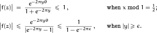
Therefore |f(z)| is bounded on the contour, and the integral is O(M^1–m). The residue of 2πif(z)/z^m at z = k ≠ 0 is e^2πikθ/k^m; the residue at z = 0 is the coefficient of z^–1 in

namely (2πi)^mB_m(θ)/m!. Therefore the sum of residues inside the contour is

This equals the contour integral O(M^1–m), so it approaches zero as M → ∞.

9.59 If F(x) is sufficiently well behaved, we have the general identity

where . (This is “Poisson’s summation formula,” which can be found in standard texts such as Henrici [182, Theorem 10.6e].)

9.60 The stated formula is equivalent to

by exercise 5.22. Hence the result follows from exercises 6.64 and 9.44.

9.61 The idea is to make α “almost” rational. Let a_k = 2^22k be the kth partial quotient of α, and let , where q_m = K(a₁, . . . , a_m) and m is even. Then 0 < {q_mα} < 1/K(a₁, . . . , a_m+1) < 1/(2n), and if we take v = a_m+1/(4n) we get a discrepancy . If this were less than n^1– we would have ; but in fact .

9.62 See Canfield [48]; see also David and Barton [71, Chapter 16] for asymptotics of Stirling numbers of both kinds.

9.63 Let c = φ^2–φ. The estimate cn^φ–1+o(n^φ–1) was proved by Fine [150]. Ilan Vardi observes that the sharper estimate stated can be deduced from the fact that the error term e(n) = f(n) – cn^φ–1 satisfies the approximate recurrence c^φn^2–φe(n) ≈ – ∑_k e(k)[1 ≤ k < cn^φ–1 ]. The function

satisfies this recurrence asymptotically, if u(x + 1) = –u(x). (Vardi conjectures that

Additional progress on this problem has been made by Jean-Luc Rémy, Journal of Number Theory, vol. 66 (1997), 1–28.

for some such function u.) Calculations for small n show that f(n) equals the nearest integer to cn^φ–1 for 1 ≤ n ≤ 400 except in one case: f(273) = 39 > c · 273^{φ –1} ≈ 38.4997. But the small errors are eventually magnified, because of results like those in exercise 2.36. For example, e(201636503) ≈ 35.73; e(919986484788) ≈ –1959.07.

9.64 (From this identity for B₂(x) we can easily derive the identity of exercise 58 by induction on m.) If 0 < x < 1, the integral can be expressed as a sum of N integrals that are each O(N^–2), so it is O(N^–1); the constant implied by this O may depend on x. Integrating the identity and letting N → ∞ now gives , a relation that Euler knew ([107] and [110, part 2, §92]). Integrating again yields the desired formula. (This solution was suggested by E. M. E. Wermuth [367]; Euler’s original derivation did not meet modern standards of rigor.)

9.65 Since a₀+a₁n^–1 +a₂n^–2 +· · · = 1+(n–1)^–1(a₀+a₁(n–1)^–1 +a₂(n– 1)^–2 + · · · ), we obtain the recurrence , which matches the recurrence for the Bell numbers. Hence a_m = ϖ_m.

A slightly longer but more informative proof can be based on the fact that 1/(n-1)…(n-m)=, by (7.47).

“The paradox is now fully established that the utmost abstractions are the true weapons with which to control our thought of concrete fact.”

—A. N. Whitehead [372]

9.66 The expected number of distinct elements in the sequence 1, f(1), f(f(1)), . . . , when f is a random mapping of {1, 2, . . . , n} into itself, is the function Q(n) of exercise 56, whose value is ; this might account somehow for the factor .

9.67 It is known that ; the constant e^–π/6 has been verified empirically to eight significant digits.

9.68 This would fail if, for example, for some integer m and some ; but no counterexamples are known.