Chapter 6. Torsion of Prismatic Bars
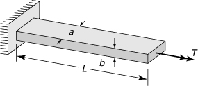
6.1 Introduction
In this chapter, consideration is given to stresses and deformations in prismatic members subject to equal and opposite end torques. In general, these bars are assumed free of end constraint. Usually, members that transmit torque, such as propeller shafts and torque tubes of power equipment, are circular or tubular in cross section. For circular cylindrical bars, the torsion formulas are readily derived employing the method of mechanics of materials, as illustrated in the next section. We shall observe that a shaft having a circular cross section is most efficient compared to a shaft having an arbitrary cross section.
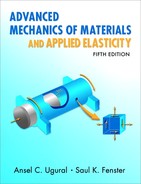
Slender members with other than circular cross sections are also often used. In treating noncircular prismatic bars, cross sections initially plane (Fig. 6.1a) experience out-of-plane deformation or warping (Fig. 6.1b), and the basic kinematic assumptions of the elementary theory are no longer appropriate. Consequently, the theory of elasticity, a general analytic approach, is employed, as discussed in Section 6.4. The governing differential equations derived using this method are applicable to both the linear elastic and the fully plastic torsion problems. The latter is treated in Section 12.10.
Figure 6.1. Rectangular bar: (a) before loading; (b) after a torque is applied.
For cases that cannot be conveniently solved analytically, the governing expressions are used in conjunction with the membrane and fluid flow analogies, as will be treated in Sections 6.6 through 6.9. Computer-oriented numerical approaches (Chap. 7) are also very efficient for such situations. The chapter concludes with discussions of warping of thin-walled open cross sections and combined torsion and bending of curved bars.
6.2 Elementary Theory of Torsion of Circular Bars
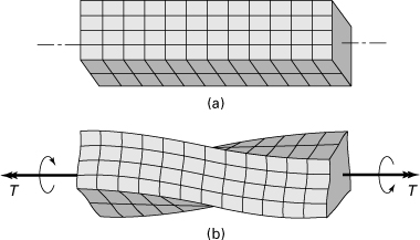
Consider a torsion bar or shaft of circular cross section (Fig. 6.2). Assume that the right end twists relative to the left end so that longitudinal line AB deforms to AB′. This results in a shearing stress τ and an angle of twist or angular deformation φ. The reader will recall from an earlier study of mechanics of materials [Ref. 6.1] the basic assumptions underlying the formulations for the torsional loading of circular bars:
1. All plane sections perpendicular to the longitudinal axis of the bar remain plane following the application of torque; that is, points in a given cross-sectional plane remain in that plane after twisting.
2. Subsequent to twisting, cross sections are undistorted in their individual planes; that is, the shearing strain γ varies linearly from zero at the center to a maximum on the outer surface.
The preceding assumptions hold for both elastic and inelastic material behavior. In the elastic case, the following also applies:
3. The material is homogeneous and obeys Hooke’s law; hence, the magnitude of the maximum shear angle γmax must be less than the yield angle.
Figure 6.2. Variation of stress and angular rotation of a circular member in torsion.
We now derive the elastic stress and deformation relationships for circular bars in torsion in a manner similar to the most fundamental equations of the mechanics of materials: by employing the previously considered procedures and the foregoing assumptions. In the case of these elementary formulas, there is complete agreement between the experimentally obtained and the computed quantities. Moreover, their validity can be demonstrated through application of the theory of elasticity (see Example 6.3).
Shearing Stress
On any bar cross section, the resultant of the stress distribution must be equal to the applied torque T (Fig. 6.2). That is,
![]()
where the integration proceeds over the entire area of the cross section. At any given section, the maximum shearing stress τmax and the distance r from the center are constant. Hence, the foregoing can be written
(a)
in which ∫ρ2dA = J is the polar moment of inertia of the circular cross section (Sec. C.2). For circle of radius r, J = πr4/2. Thus,
(6.1)
This is the well-known torsion formula for circular bars. The shearing stress at a distance ρ from the center is
(6.2)
The transverse shearing stress obtained by Eq. (6.1) or (6.2) is accompanied by a longitudinal shearing stress of equal value, as shown on a surface element in the figure.
We note that, when a shaft is subjected to torques at several points along its length, the internal torques will vary from section to section. A graph showing the variation of torque along the axis of the shaft is called the torque diagram. That is, this diagram represents a plot of the internal torque T versus its position x along the shaft length. As a sign convention, T will be positive if its vector is in the direction of a positive coordinate axis. However, the diagram is not used commonly, because in practice, only a few variations in torque occur along the length of a given shaft.
Angle of Twist
According to Hooke’s law, γmax = τmax/G; introducing the torsion formula, γmax = Tr/JG, where G is the modulus of elasticity in shear. For small deformations, tan γmax = γmax, and we may write γmax = rφ/L (Fig. 6.2). The foregoing expressions lead to the angle of twist, the angle through which one cross section of a circular bar rotates with respect to another:
(6.3)
Angle φ is measured in radians. The product JG is termed the torsional rigidity of the member. Note that Eqs. (6.1) through (6.3) are valid for both solid and hollow circular bars; this follows from the assumptions used in the derivations. For a circular tube of inner radius ri and outer radius ro, we have ![]() .
.
Example 6.1. Stress and Deformation in an Aluminum Shaft
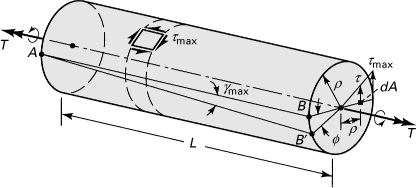
A hollow aluminum alloy 6061-T6 shaft of outer radius c = 40 mm, inner radius b = 30 mm, and length L = 1.2 m is fixed at one end and subjected to a torque T at the other end, as shown in Fig. 6.3. If the shearing stress is limited to τmax = 140 MPa, determine (a) the largest value of the torque; (b) the corresponding minimum value of shear stress; (c) the angle of twist that will create a shear stress τmin = 100 MPa on the inner surface.
Figure 6.3. Example 6.1. A tubular circular bar in torsion.
Solution
From Table D.1, we have the shear modulus of elasticity G = 72 GPa and τyp = 220 MPa.
a. Inasmuch as τmax < τyp, we can apply Eq. (6.1) with r = c to obtain
(b)
By Table C.1, the polar moment of inertia of the hollow circular tube is
![]()
Inserting J and τmax into Eq. (b) results in
![]()
b. The smallest value of the shear stress takes place on the inner surface of the shaft, and τmin and τmax are respectively proportional to b and c. Therefore,
![]()
c. Through the use of Eq. (2.27), the shear strain on the inner surface of the shaft is equal to
![]()
Referring to Fig. 6.2,
![]()
or
φ = 3.19°
Example 6.2. Redundantly Supported Shaft
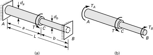
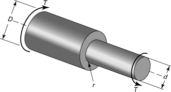
A solid circular shaft AB is fixed to rigid walls at both ends and subjected to a torque T at section C, as shown in Fig. 6.4a. The shaft diameters are da and db for segments AC and CB, respectively. Determine the lengths a and b if the maximum shearing stress in both shaft segments is to be the same for da = 20 mm, db = 12 mm, and L = 600 mm.
Figure 6.4. Example 6.2. (a) A fixed-ended circular shaft in torsion; (b) free-body diagram of the entire shaft.
Solution
From the free-body diagram of Fig. 6.4a, we observe that the problem is statically indeterminate to the first degree; the one equation of equilibrium available is not sufficient to obtain the two unknown reactions TA and TB.
Condition of Equilibrium. Using the free-body diagram of Fig. 6.4b,
(c)
Torque-Displacement Relations. The angle of twist at section C is expressed in terms of the left and right segments of the solid shaft, respectively, as
(d)
Here, the polar moments of inertia are ![]() and
and ![]() .
.
Condition of Compatibility. The two segments must have the same angle of twist where they join. Thus,
(e)
Equations (c) and (e) can be solved simultaneously to yield the reactions
(f)
The maximum shearing stresses in each segment of the shaft are obtained from the torsion formula:
(g)
For the case under consideration, τa = τb, or
![]()
Introducing Eqs. (f) into the foregoing and simplifying, we obtain
![]()
from which
(h)
where L = a + b. Insertion of the given data results in
![]()
For a prescribed value of torque T, we can now compute the reactions, angle of twist at section C, and maximum shearing stress from Eqs. (f), (d), and (g), respectively.
Axial and Transverse Shear Stresses
In the foregoing, we considered shear stresses acting in the plane of a cut perpendicular to the axis of the shaft, defined by Eqs. (6.1) and (6.2). Their directions coincide with the direction of the internal torque T on the cross section (Fig. 6.2). These stresses must be accompanied by equal shear stresses occurring on the axial planes of the shaft, since equal shear stresses always exist on mutually perpendicular planes.
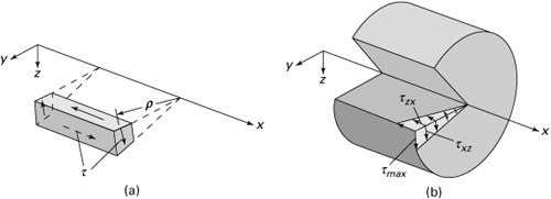
Consider the state of stress as depicted in Fig. 6.5a. Note that τ is the only stress component acting on this element removed from the bar; the element is in the state of pure shear. Observe that τ = τxz = τzx denotes the shear stresses in the tangential and axial directions. So, the internal torque develops not only a transverse shear stress along radial lines or in the cross section but also an associated axial shear stress distribution along a longitudinal plane. The variation of these stresses on the mutually perpendicular planes is illustrated in Fig. 6.5b, where a portion of the shaft has been removed for the purposes of illustration. Consequently, if a material is weaker in shear axially than laterally (such as wood), the failure in a twisted bar occurs longitudinally along axial planes.
Figure 6.5. Shearing stresses on transverse (xz) and axial (zx) planes of a shaft (Fig. 6.2): (a) shaft element in pure shear; (b) shaft segment in pure shear.
6.3 Stresses on Inclined Planes
Our treatment thus far has been limited to shearing stresses on planes at a point parallel or perpendicular to the axis of a shaft, defined by the torsion formula. This state of stress is depicted acting on a surface element on the left of the shaft in Fig. 6.6a. Alternatively, representation of the stresses at the same point may be given on an infinitesimal two-dimensional wedge whose outer normal (x′) on its oblique face makes an angle θ with the axial axis (x), as shown in Fig. 6.6b.
Figure 6.6. (a) Stresses acting on the surface elements of a shaft in torsion; (b) free-body diagram of wedge cut from the shaft; (c) Mohr’s circle for torsional loading.
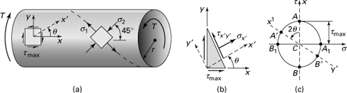
We shall analyze the stresses σx′ and τx′y′ that must act on the inclined plane to keep the isolated body, as discussed in Sections 1.7 and 1.9. The equilibrium conditions of forces in the x′ and y′ directions, Eqs. (1.18a and 1.18b) with σx = σy = 0 and τxy = –τmax, give
(6.4a)
(6.4b)
These are the equations of transformation for stress in a shaft under torsion.
Figure 6.6c, a Mohr’s circle for torsional loading provides a convenient way of checking the preceding results. Observe that the center C of the circle is at the origin of the coordinates σ and τ. It is recalled that points A′ and B′ define the states of stress about any other set of x′ and y′ planes relative to the set through an angle θ. Similarly, the points A(0, τmax) and B(0, τmin) are located on the τ axis, while A1 and B1 define the principal planes and the principal stresses. The radius of the circle is equal to the magnitude of the maximum shearing stress.
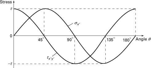
The variation in the stresses σx′ and σx′y′ with the orientation of the inclined plane is demonstrated in Fig. 6.7. It is seen that τmax = τ and τx′y′ = 0 when θ = 45° and σmin = –τ, and τx′y′ = 0 when θ = 135°. That is, the maximum normal stress equals σ1 = Tr/J, and the minimum normal stress equals σ2 = –Tr/J, acting in the directions shown in Fig. 6.6a. Also, no shearing stress greater than τ is developed.
Figure 6.7. Graph of normal stress σx′ and shear stress τx′y′ versus angle θ of the inclined plane.
It is clear that, for a brittle material such as cast iron, which is weaker in tension than in shear, failure occurs in tension along a helix as indicated by the dashed lines in Fig. 6.6a. Ordinary chalk behaves in this manner. On the contrary, shafts made of ductile materials weak in shearing strength (for example, mild steel) break along a line perpendicular to the axis. The preceding is consistent with the types of tensile failures discussed in Section 2.7.
6.4 General Solution of the Torsion Problem
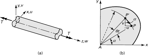
Consider a prismatic bar of constant arbitrary cross section subjected to equal and opposite twisting moments applied at the ends, as in Fig. 6.8a. The origin of x, y, and z in the figure is located at the center of twist of the cross section, about which the cross section rotates during twisting. It is sometimes defined as the point at rest in every cross section of a bar in which one end is fixed and the other twisted by a couple. At this point, u and v, the x and y displacements, are thus zero. The location of the center of twist is a function of the shape of the cross section. Note that while the center of twist is referred to in the derivations of the basic relationships, it is not dealt with explicitly in the solution of torsion problems (see Prob. 6.19). The z passes through the centers of twist of all cross sections.
Figure 6.8. Torsion member of arbitrary cross section.
Geometry of Deformation
In general, the cross sections warp, as already noted. We now explore the problem of torsion with free warping, applying the Saint-Venant semi-inverse method [Refs. 6.2 and 6.3]. As a fundamental assumption, the warping deformation is taken to be independent of axial location, that is, identical for any cross section:
(a)
It is also assumed that the projection on the xy plane of any warped cross section rotates as a rigid body and that the angle of twist per unit length of the bar, θ, is constant.
We refer now to Fig. 6.8b, which shows the partial end view of the bar (and could represent any section). An arbitrary point on the cross section, point P(x, y), located a distance r from center of twist A, has moved to P′ = (x – u, y + v) as a result of torsion. Assuming that no rotation occurs at end z = 0 and that θ is small, the x and y displacements of P are, respectively,
(b)
where the angular displacement of AP at a distance z from the left end is θz; then x, y, and z are the coordinates of point P, and α is the angle between AP and the x axis. Clearly, Eqs. (b) specify the rigid body rotation of any cross section through a small angle θz. By substituting Eqs. (a) and (b) into Eq. (2.4), we have
(c)
Equation (2.36) together with this expression leads to the following:
(d)
(e)
Equations of Equilibrium
By now substituting Eq. (d) into the equations of equilibrium (1.14), assuming negligible body forces, we obtain
(6.5)
Equations of Compatibility
Differentiating the first equation of (e) with respect to y and the second with respect to x and subtracting the second from the first, we obtain an equation of compatibility:
(6.6)
where
(6.7)
The stress in a bar of arbitrary section may thus be determined by solving Eqs. (6.5) and (6.6) along with the given boundary conditions.
6.5 Prandtl’s Stress Function
As in the case of beams, the torsion problem formulated in the preceding is commonly solved by introducing a single stress function. If a function Φ(x, y), the Prandtl stress function, is assumed to exist, such that
(6.8)
then the equations of equilibrium (6.5) are satisfied. The equation of compatibility (6.6) becomes, upon substitution of Eq. (6.8),
(6.9)
The stress function Φ must therefore satisfy Poisson’s equation if the compatibility requirement is to be satisfied.
Boundary Conditions
We are now prepared to consider the boundary conditions, treating first the load-free lateral surface. Recall from Section 1.5 that τxz is a z-directed shearing stress acting on a plane whose normal is parallel to the x axis, that is, the yz plane. Similarly, τzx acts on the xy plane and is x-directed. By virtue of the symmetry of the stress tensor, we have τxz = τzx and τyz = τzy. Therefore, the stresses given by Eq. (e) may be indicated on the xy plane near the boundary, as shown in Fig. 6.9. The boundary element is associated with arc length ds. Note that ds increases in the counterclockwise direction. When ds is zero, the element represents a point at the boundary. Then, referring to Fig. 6.9 together with Eq. (1.48), which relates the surface forces to the internal stress, and noting that the cosine of the angle between z and a unit normal n to the surface is zero [that is, cos(n, z) = 0], we have
(a)
Figure 6.9. Arbitrary cross section of a prismatic member in torsion.
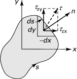
According to Eq. (a), the resultant shear stress τ must be tangent to the boundary (Fig. 6.9). From the figure, it is clear that
(b)
Note that as we proceed in the direction of increasing s, x decreases and y increases. This accounts for the algebraic sign in front of dx and dy in Fig. 6.9. Substitution of Eqs. (6.8) and (b) into Eq. (a) yields
(6.10)
This expression states that the directional deviation along a boundary curve is zero. Thus, the function Φ(x, y) must be an arbitrary constant on the lateral surface of the prism. Examination of Eq. (6.8) indicates that the stresses remain the same regardless of additive constants; that is, if Φ + constant is substituted for Φ, the stresses will not change. For solid cross sections, we are therefore free to set Φ equal to zero at the boundary. In the case of multiply connected cross sections, such as hollow or tubular members, an arbitrary value may be assigned at the boundary of only one of the contours s0, s1,..., sn. For such members it is necessary to extend the mathematical formulation presented in this section. Solutions for thin-walled, multiply connected cross sections are treated in Section 6.8 by use of the membrane analogy.
Returning to the member of solid cross section, we complete discussion of the boundary conditions by considering the ends, at which the normals are parallel to the z axis and therefore cos(n, z) = n = ± 1, l = m = 0. Equation (1.48) now gives, for pz = 0,
(c)
where the algebraic sign depends on the relationship between the outer normal and the positive z direction. For example, it is negative for the end face at the origin in Fig. 6.8a.
We now confirm that the summation of forces over the ends of the bar is zero:
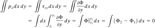
Here y1 and y2 represent the y coordinates of points located on the surface. Inasmuch as Φ = constant on the surface of the bar, the values of Φ corresponding to y1 and y2 must be equal to a constant, Φ1 = Φ2 = constant. Similarly it may be shown that
![]()
The end forces, while adding to zero, must nevertheless provide the required twisting moment or externally applied torque about the z axis:
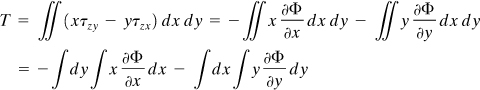
Integrating by parts,
![]()
Since Φ = constant at the boundary and x1, x2, y1, and y2 denote points on the lateral surface, it follows that
(6.11)
Inasmuch as Φ(x, y) has a value at each point on the cross section, it is clear that Eq. (6.11) represents twice the volume beneath the Φ surface.
What has resulted from the foregoing development is a set of equations satisfying all the conditions of the prescribed torsion problem. Equilibrium is governed by Eqs. (6.8), compatibility by Eq. (6.9), and the boundary condition by Eq. (6.10). Torque is related to stress by Eq. (6.11). To ascertain the distribution of stress, it is necessary to determine a stress function that satisfies Eqs. (6.9) and (6.10), as is demonstrated in the following example.
Example 6.3. Analysis of an Elliptical Torsion Bar
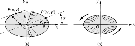
Consider a solid bar of elliptical cross section (Fig. 6.10a). Determine the maximum shearing stress and the angle of twist per unit length. Also, derive an expression for the warping w(x, y).
Figure 6.10. Example 6.3. Elliptical cross section: (a) shear stress distribution; (b) out-of plane deformation or warping.
Solution
Equations (6.9) and (6.10) are satisfied by selecting the stress function
![]()
where k is a constant. Substituting this into Eq. (6.9), we obtain
![]()
Hence,
(d)
and Eq. (6.11) yields
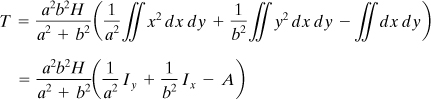
where A is the cross-sectional area. Inserting expressions for Ix, Iy, and A (Table C.1) results in
(e)
from which
(f)
The stress function is now expressed as
![]()
and the shearing stresses are found readily from Eq. (6.8):
(g)
The ratio of these stress components is proportional to y/x and thus constant along any radius of the ellipse:
![]()
The resultant shearing stress,
(h)
has a direction parallel to a tangent drawn at the boundary at its point of intersection with the radius containing the point under consideration. Note that α represents an arbitrary angle (Fig. 6.10a).
To determine the location of the maximum resultant shear, which from Eq. (g) is somewhere on the boundary, consider a point P′(x′, y′) located on a diameter conjugate to that containing P(x, y) (Fig. 6.10a). Note that OP′ is parallel to the tangent line at P. The coordinates of P and P′ are related by
![]()
When these expressions are substituted into Eq. (h), we have
(i)
Clearly, τzα will have its maximum value corresponding to the largest value of the conjugate semidiameter r′. This occurs where r′ = a or r = b. The maximum resultant shearing stress thus occurs at P(x, y), corresponding to the extremities of the minor axis as follows: x = 0, y = ± b. From Eq. (i),
(6.12a)
The angle of twist per unit length is obtained by substituting Eq. (f) into Eq. (6.7):
(6.12b)
We note that the factor by which the twisting moment is divided to determine the twist per unit length is called the torsional rigidity, commonly denoted C. That is,
(6.13)
The torsional rigidity for an elliptical cross section, from Eq. (6.12b), is thus
![]()
Here A = πab and J = πab(a2 + b2)/4 are the area and polar moment of inertia of the cross section.
The components of displacement u and v are then found from Eq. (b) of Section 6.4. To obtain the warpage w(x, y), consider Eq. (e) of Section 6.4 into which have been substituted the previously derived relations for τzx, τzy, and θ:
Integration of these equations leads to identical expressions for w(x, y), except that the first also yields an arbitrary function of y, f(y), and the second an arbitrary function of x, f(x). Since w(x, y) must give the same value for a given P(x, y), we conclude that f(x) = f(y) = 0; what remains is
(6.14)
The contour lines, obtained by setting w = constant, are the hyperbolas shown in Fig. 6.10b. The solid lines indicate the portions of the section that become convex, and the dashed lines indicate the portions of the section that become concave when the bar is subjected to a torque in the direction shown.
Circular Cross Section
The results obtained in this example for an elliptical section may readily be reduced to the case of a circular section by setting a and b equal to the radius of a circle r (Fig. 6.6a). Equations (6.12a and b) thus become
![]()
where the polar moment of inertia, J = πr4/2. Similarly, Eq. (6.14) gives w = 0, verifying assumption (1) of Section 6.2.
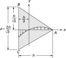
Example 6.4. Equilateral Triangle Bar under Torsion
An equilateral cross-sectional solid bar is subjected to pure torsion (Fig. 6.11). What are the maximum shearing stress and the angle of twist per unit length?
Figure 6.11. Example 6.4. Equilateral triangle cross section.
Solution
The equations of the boundaries are expressed as
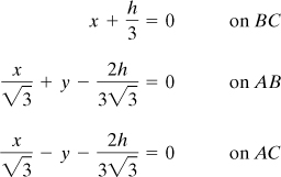
Therefore, the stress function that vanishes at the boundary may be written in the form:
(j)
in which k is constant.
Proceeding as in Example 6.3, it can readily be shown (see Prob. 6.23) that the largest shearing stress at the middle of the sides of the triangle is equal to
(k)
At the corners of the triangle, the shearing stress is zero, as shown in Fig. 6.11. Angle of twist per unit length is given by
(l)
The torsional rigidity is therefore ![]() . Note that, for an equilateral triangle of sides a, we have
. Note that, for an equilateral triangle of sides a, we have ![]() . (Fig. 6.11).
. (Fig. 6.11).
Example 6.5. Rectangular Bar Subjected to Torsion
A torque T acts on a bar having rectangular cross section of sides a and b (Fig. 6.12). Outline the derivations of the expressions for the maximum shearing stress τmax and the angle of twist per unit length θ.
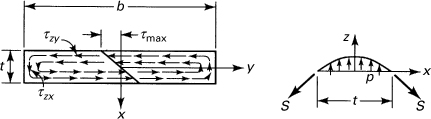
Figure 6.12. Example 6.5. Shear stress distribution in the rectangular cross section of atorsion bar.
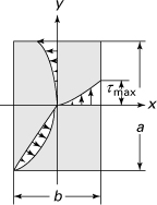
Solution
The indirect method employed in the preceding examples does not apply to the rectangular cross sections. Mathematical solution of the problem is lengthy. For situations that cannot be conveniently solved by applying the theory of elasticity, the governing equations are used in conjunction with the experimental methods, such as membrane analogy (Ref. 6.4). Finite element analysis is also very efficient for this purpose.
The shear stress distribution along three radial lines initiating from the center of a rectangular section of a bar in torsion are shown in Fig. 6.12, where the largest stresses are along the center line of each face. The difference in this stress distribution compared with that of a circular section is very clear. For the latter, the stress is a maximum at the most remote point, but for the former, the stress is zero at the most remote point. The values of the maximum shearing stress τmax in a rectangular cross section and the angle of twist per unit length θ are given in the next section (see Table 6.2).
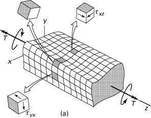
Interestingly, a corner element of the cross section of a rectangular shaft under torsion does not distort at all, and hence the shear stresses are zero at the corners, as illustrated in Fig. 6.13. This is possible because outside surfaces are free of all stresses. The same considerations can be applied to the other points on the boundary. The shear stresses acting on three outermost cubic elements isolated from the bar are illustrated in the figure. Here stress-free surfaces are indicated as shaded. Observe that all shear stresses τxy and τxz in the plane of a cut near the boundaries act on them.
Figure 6.13. Example 6.5. Deformation and stress in a rectangular bar segment under torsion. Note that the original plane cross sections have warped out of their own plane.
6.6 Prandtl’s Membrane Analogy
It is demonstrated next that the differential equation for the stress function, Eq. (6.9), is of the same form as the equation describing the deflection of a membrane or soap film subject to pressure. Hence, an analogy exists between the torsion and membrane problems, serving as the basis of a number of experimental techniques. Consider an edge-supported homogeneous membrane, given its boundary contour by a hole cut in a plate (Fig. 6.14a). The shape of the hole is the same as that of the twisted bar to be studied; the sizes need not be identical.
Figure 6.14. Membrane analogy for torsion members of solid cross section.
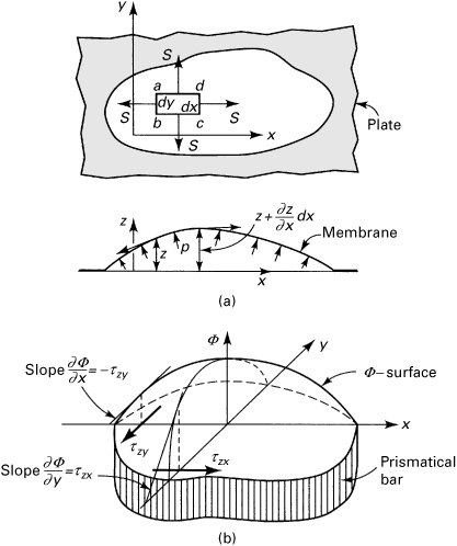
Equation of Equilibrium
The equation describing the z deflection of the membrane is derived from considerations of equilibrium applied to the isolated element abcd. Let the tensile forces per unit membrane length be denoted by S. From a small z deflection, the inclination of S acting on side ab may be expressed as β ≈ ∂z/∂x. Since z varies from point to point, the angle at which S is inclined on side dc is
![]()
Similarly, on sides ad and bc, the angles of inclination for the tensile forces are ∂z/∂y and ∂z/∂y + (∂2z/∂y2) dy, respectively. In the development that follows, S is regarded as a constant, and the weight of the membrane is ignored. For a uniform lateral pressure p, the equation of vertical equilibrium is then
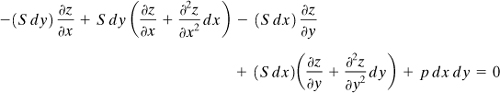
(6.15)
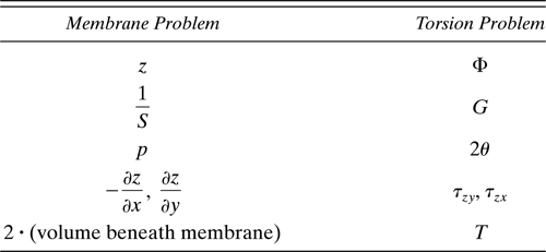
This is again Poisson’s equation. Upon comparison of Eq. (6.15) with Eqs. (6.9) and (6.8), the quantities shown in Table 6.1 are observed to be analogous. The membrane, subject to the conditions outlined, thus represents the Φ surface (Fig. 6.14b). In view of the derivation, the restriction with regard to smallness of slope must be borne in mind.
Table 6.1. Analogy between Membrane and Torsion Problems
Shearing Stress and Angle of Twist
We outline next one method by which the foregoing theory can be reduced to a useful experiment. In two thin, stiff plates, bolted together, are cut two adjacent holes; one conforms to the outline of the irregular cross section and the other is circular. The plates are then separated and a thin sheet of rubber stretched across the holes (with approximately uniform and equal tension). The assembly is then bolted together. Subjecting one side of the membrane to a uniform pressure p causes a different distribution of deformation for each cross section, with the circular hole providing calibration data. The measured geometric quantities associated with the circular hole, together with the known solution, provide the needed proportionalities between pressure and angle of twist, slope and stress, volume and torque. These are then applied to the irregular cross section, for which the measured slopes and volume yield τ and T. The need for precise information concerning the membrane stress is thus obviated.
The membrane analogy provides more than a useful experimental technique. As is demonstrated in the next section, it also serves as the basis for obtaining approximate analytical solutions for bars of narrow cross section as well as for members of open thin-walled section.
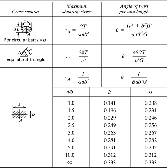
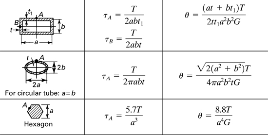
For reference purposes, Table 6.2 presents the shearing stress and angle of twist for a number of commonly encountered shapes [Ref. 6.4]. Note that the values of coefficients α and β depend on the ratio of the length of the long side or depth a to the width b of the short side of a rectangular section. For thin sections, where a is much greater than b, their values approach 1/3. We observe that, in all cases, the maximum shearing stresses occur at a point on the edge of the cross section that is closest to the center axis of the shaft. A circular shaft is the most efficient; it is subjected to both smaller maximum shear stress and a smaller angle of twist than the corresponding noncircular shaft of the same cross-sectional area and carrying the same torque.
Table 6.2. Shear Stress and Angle of Twist of Various Members in Torsion
Example 6.6. Analysis of a Stepped Bar in Torsion
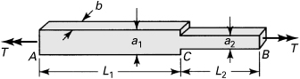
A rectangular bar of width b consists of two segments: one with depth a1 = 60 mm and length L1 = 2.5 m and the other with depth a2 = 45 mm and length L2 = 1.5 m (Fig. 6.15). The bar is to be designed using an allowable shearing stress τall = 50 MPa and an allowable angle of twist per unit length θall = 1.5° per meter. Determine (a) the maximum permissible applied torque Tmax, assuming b = 30 mm and G = 80 GPa, and (b) the corresponding angle of twist between the end sections, φmax.
Figure 6.15. Example 6.6. A stepped rectangular torsion bar.
Solution
The values of the torsion parameters from Table 6.2 are
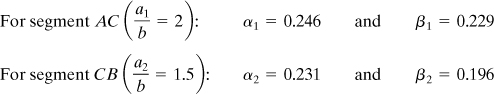
a. Segment BC governs because it is of smaller depth. The permissible torque T based on the allowable shearing stress is obtained from τmax = T/αab2. Thus,
T = α2a2b2τmax = 0.231(0.045)(0.03)2(50 × 106) = 468 N · m
The allowable torque T corresponding to the allowable angle of twist per unit length is determined from θ = T/βab3G:
![]()
The maximum permissible torque, equal to the smaller of the two preceding values, is Tmax = 468 N · m.
b. The angle of twist is equal to the sum of the angles of twist for the two segments:
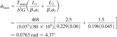
Clearly, had the allowable torque been based on the angle of twist per unit length, we would have found that φmax = θall(L1 + L2) = 1.5(4) = 6°.
6.7 Torsion of Narrow Rectangular Cross Section
In applying the analogy to a bar of narrow rectangular cross section, it is usual to assume a constant cylindrical membrane shape over the entire dimension b (Fig. 6.16). Subject to this approximation, ∂z/∂y = 0, and Eq. (6.15) reduces to d2z/dx2 = –p/S, which is twice integrated to yield the parabolic deflection
(a)
Figure 6.16. Membrane analogy for a torsional member of narrow rectangular cross section.
To arrive at Eq. (a), the boundary conditions that dz/dx = 0 at x = 0 and z = 0 at x = t/2 have been employed. The volume bounded by the parabolic cylindrical membrane and the xy plane is given by V = pbt3/12S. According to the analogy, p is replaced by 2θ and 1/S by G, and consequently ![]() . The torsional rigidity for a thin rectangular section is therefore
. The torsional rigidity for a thin rectangular section is therefore
(6.16)
Here Je represents the effective polar moment of inertia of the section. The analogy also requires that
(b)
The angle of twist per unit length is, from Eq. (6.16),
(6.17)
Maximum shear occurs at ±t/2 is
(6.18)
(6.19)
According to Eq. (b), the shearing stress is linear in x, as in Fig. 6.9, producing a twisting moment T about z given by
![]()
This is exactly one-half the torque given by Eq. (6.19). The remaining applied torque is evidently resisted by the shearing stresses τzx, neglected in the original analysis in which the membrane is taken as cylindrical. The membrane slope at y = ±b/2 is smaller than that at x = ±t/2 or, equivalently, (τzx)max < (τzy)max. It is clear, therefore, that Eq. (6.18) represents the maximum shearing stress in the bar, of a magnitude unaffected by the original approximation. That the lower τzx stresses can provide a resisting torque equal to that of the τzy stresses is explained on the basis of the longer moment arm for the stresses near y = ±b/2.
Thin-Walled Open Cross Sections
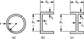
Equations (6.17) and (6.18) are also applicable to thin-walled open sections such as those shown in Fig. 6.17. Because the foregoing expressions neglect stress concentration, the points of interest should be reasonably distant from the corners of the section (Figs. 6.17b and c). The validity of the foregoing approach depends on the degree of similarity between the membrane shape of Fig. 6.16 and that of the geometry of the component section. Consider, for example, the I-section of Fig. 6.17c. Because the section is of varying thickness, the effective polar moment of inertia is written as
(6.20)
Figure 6.17. Thin-walled open sections.
or
![]()
(6.21a)
(6.21b)
where ti is the larger of t1 and t2. The effect of the stress concentrations at the corners will be examined in Section 6.9.
6.8 Torsion of Multiply Connected Thin-Walled Sections
The membrane analogy may be applied to good advantage to analyze the torsion of thin tubular members, provided that some care is taken. Consider the deformation that would occur if a membrane subject to pressure were to span a hollow tube of arbitrary section (Fig. 6.18a). Since the membrane surface is to describe the stress function (and its slope, the stress at any point), arc ab cannot represent a meaningful stress function. This is simply because in the region ab the stress must be zero, because no material exists there. If the curved surface ab is now replaced by a plane representing constant Φ, the zero-stress requirement is satisfied. For bars containing multiply connected regions, each boundary is also a line of constant Φ of different value. The absolute value of Φ is meaningless, and therefore at one boundary, Φ may arbitrarily be equated to zero and the others adjusting accordingly.
Figure 6.18. Membrane analogy for tubular torsion members: (a) and (b) one-cell section; (c) two-cell section.
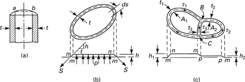
Shearing Stress
Based on the foregoing considerations, the membrane analogy is extended to a thin tubular member (Fig. 6.18b), in which the fixed plate to which the membrane is attached has the same contour as the outer boundary of the tube. The membrane is also attached to a “weightless” horizontal plate having the same shape as the inner boundary nn of the tube, thus bridging the inner and outer contours over a distance t. The inner horizontal plate, made “weightless” by a counterbalance system, is permitted to seek its own vertical position but is guided so as not to experience sideward motion. Because we have assumed the tube to be thin walled, the membrane curvature may be disregarded; that is, lines nn may be considered straight. We are thus led to conclude that the slope is constant over a given thickness t, and consequently the shearing stress is likewise constant, given by
(a)
where h is the membrane deflection and t the tube thickness. Note that the tube thickness may vary circumferentially.
The dashed line in Fig. 6.18b indicates the mean perimeter, which may be used to determine the volume bounded by the membrane. Letting A represent the area enclosed by the mean perimeter, the volume mnnm is simply Ah, and the analogy gives
(b)
Combining Eqs. (a) and (b), we have
(6.22)
The application of Eq. (6.22) is limited to thin-walled members displaying no abrupt variations in thickness and no reentrant corners in their cross sections.
Angle of Twist
To develop a relationship for the angle of twist from the membrane analogy, we again consider Fig. 6.18b, in which h ≪ t and consequently tan(h/t) ≈ h/t = τ. Vertical equilibrium therefore yields
![]()
Here s is the length of the mean perimeter of the tube. Since the membrane tension is constant, h is independent of S. The preceding is then written
![]()
where the last term follows from the analogy. The angle of twist per unit length is now found directly:
(6.23)
Equations (6.22) and (6.23) are known as Bredt’s formulas.
In Eqs. (a), (b), and (6.23), the quantity h possesses the dimensions of force per unit length, representing the resisting force per unit length along the tube perimeter. For this reason, h is referred to as the shear flow.
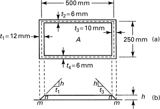
Example 6.7. Rectangular Torsion Tube
An aluminum tube of rectangular cross section (Fig. 6.19a) is subjected to a torque of 56.5 kN · m along its longitudinal axis. Determine the shearing stresses and the angle of twist. Assume G = 28 GPa.
Figure 6.19. Example 6.7. (a) Cross section; (b) membrane.
Solution
Referring to Fig. 6.19b, which shows the membrane surface mnnm (representing Φ), the applied torque is, according to Eq. (b),
T = 2Ah = 2(0.125h) = 56,500 N · m
from which h = 226,000 N/m. The shearing stresses are found from Eq. (a) as follows:
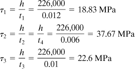
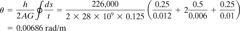
Applying Eq. (6.23), the angle of twist per unit length is
If multiply connected regions exist within a tubular member, as in Fig. 6.18c, the foregoing techniques are again appropriate. As before, the thicknesses are assumed small, so lines such as mn, np, and pm are regarded as straight. The stress function is then represented by the membrane surface mnnppm. As in the case of a simple hollow tube, lines nn and pp are straight by virtue of flat, weightless plates with contours corresponding to the inner openings. Referring to the figure, the shearing stresses are
(c)
(d)
The stresses are produced by a torque equal to twice the volume beneath surface mnnppm,
(e)
or, upon substitution of Eqs. (c),
(f)
Assuming the thicknesses t1, t2, and t3 constant, application of Eq. (6.23) yields
(g)
(h)
where s1, s2, and s3 represent the paths of integration indicated by the dashed lines. Note the relationship among the algebraic sign, the assumed direction of stress, and the direction in which integration proceeds. There are thus four equations [(d), (f), (g), and (h)] containing four unknowns: τ1, τ2, τ3, and θ.
If now Eq. (d) is written in the form
(i)
it is observed that the shear flow h = τt is constant and distributes itself in a manner analogous to a liquid circulating through a channel of shape identical with that of the tubular bar. This analogy proves very useful in writing expressions for shear flow in tubular sections of considerably greater complexity.
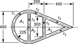
Example 6.8. Three-Cell Torsion Tube
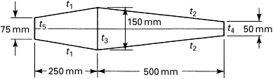
A multiply connected steel tube (Fig. 6.20) resists a torque of 12 kN · m. The wall thicknesses are t1 = t2 = t3 = 6 mm and t4 = t5 = 3 mm. Determine the maximum shearing stresses and the angle of twist per unit length. Let G = 80 GPa. Dimensions are given in millimeters.
Figure 6.20. Example 6.8. Three-cell section.
Solution
Assuming the shearing stresses directed as shown, consideration of shear flow yields
(j)
The torque associated with the shearing stresses must resist the externally applied torque, and an expression similar to Eq. (f) is obtained:
(k)
Three more equations are available through application of Eq. (6.23) over areas A1, A2, and A3:
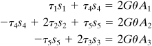
(l)
Here, s1 = 0.7069 m, s2 = 0.2136 m, s3 = 0.4272 m, s4 = 0.45 m, s5 = 0.3 m, A1 = 0.079522 m2, A2 = 0.075 m2, and A3 = 0.06 m2. There are six equations in the five unknown stresses and the angle of twist per unit length. Thus, simultaneous solution of Eqs. (j), (k), and (l) leads to the following rounded values: τ1 = 4.902 MPa, τ2 = 5.088 MPa, τ3 = 3.809 MPa, τ4 = –0.373 MPa, τ5 = 2.558 MPa, and θ = 0.0002591 rad/m. The positive values obtained for τ1, τ2, τ3, and τ5 indicate that the directions of these stresses have been correctly assumed in Fig. 6.20. The negative sign of τ4 means that the direction initially assumed was incorrect; that is, τ4 is actually upward directed.
6.9 Fluid Flow Analogy and Stress Concentration
Examination of Eq. 6.8 suggests a similarity between the stress function Φ and the stream function ψ of fluid mechanics:
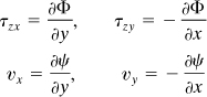
(6.24)
In Eqs. (6.24), vx and vy represent the x and y components of the fluid velocity v. Recall that, for an incompressible fluid, the equation of continuity may be written
Continuity is thus satisfied when ψ(x, y) is defined as in Eqs. (6.24). The vorticity ![]() is for two-dimensional flow,
is for two-dimensional flow,
![]()
where ∇ = (∂/∂x)i + (∂/∂y)j. In terms of the stream function, we obtain
(6.25)
The expression is clearly analogous to Eq. (6.9) with –2ω replacing –2Gθ. The completeness of the analogy is assured if it can be demonstrated that ψ is constant along a streamline (and hence on a boundary), just as Φ is constant over a boundary. Since the equation of a streamline in two-dimensional flow is
![]()
in terms of the stream function, we have
(6.26)
This is simply the total differential dψ, and therefore ψ is constant along a streamline.
Based on the foregoing, experimental techniques have been developed in which the analogy between the motion of an ideal fluid of constant vorticity and the torsion of a bar is successfully exploited. The tube in which the fluid flows and the cross section of the twisted member are identical in these experiments and useful in visualizing stress patterns in torsion. Moreover, a vast body of literature exists that deals with flow patterns around bodies of various shapes, and the results presented are often directly applicable to the torsion problem.
The fluid flow or hydrodynamic analogy is especially valuable in dealing with stress concentration in shear, which we have heretofore neglected. In this regard, consider first the torsion of a circular bar containing a small circular hole (Fig. 6.21a). Figure 6.21b shows the analogous flow pattern produced by a solid cylindrical obstacle placed in a circulating fluid. From hydrodynamic theory, it is found that the maximum velocity (at points a and b) is twice the value in the undisturbed stream at the respective radii. From this, it is concluded that a small hole has the effect of doubling the shearing stress normally found at a given radius.
Figure 6.21. (a) Circular shaft with hole; (b) fluid-flow pattern around small cylindrical obstacle; (c) circular shaft with keyway.
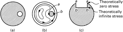
Of great importance also is the shaft keyway shown in Fig. 6.21c. According to the hydrodynamic analogy, the points a ought to have zero stress, since they are stagnation points of the fluid stream. In this sense, the material in the immediate vicinity of points a is excess. On the other hand, the velocity at the points b is theoretically infinite and, by analogy, so is the stress. It is therefore not surprising that most torsional fatigue failures have their origins at these sharp corners, and the lesson is thus supplied that it is profitable to round such corners.
6.10 Torsion of Restrained Thin-Walled Members of Open Cross Section
It is a basic premise of previous sections of this chapter that all cross sections of a bar subject to torques applied at the ends suffer free warpage. As a consequence, we must assume that the torque is produced by pure shearing stresses distributed over the ends as well as all other cross sections of the member. In this way, the stress distribution is obtained from Eq. (6.9) and satisfies the boundary conditions, Eq. (6.10).
If any section of the bar is held rigidly, it is clear that the rate of change of the angle of twist as well as the warpage will now vary in the longitudinal direction. The longitudinal fibers are therefore subject to tensile or compressive stresses. Equations (6.9) and (6.10) are, in this instance, applied with satisfactory results in regions away from the restrained section of the bar. While this restraint has negligible influence on the torsional resistance of members of solid section such as rectangles and ellipses, it is significant when dealing with open thin-walled sections such as channels of I-beams. Consider, for example, the case of a cantilever I-beam, shown in Fig. 6.22a. The applied torque causes each cross section to rotate about the axis of twist (z), thereby resulting in bending of the flanges. According to beam theory, the associated bending stresses in the flanges are zero at the juncture with the web. Consequently, the web does not depart from a state of simple torsion. In resisting the bending of the flanges or the warpage of a cross section, considerable torsional stiffness can, however, be imparted to the beam.
Figure 6.22. I-section torsion member: (a) warping is prevented of the section at x = 0; (b) partly lateral shear and partly torsional shear at arbitrary cross section AB.
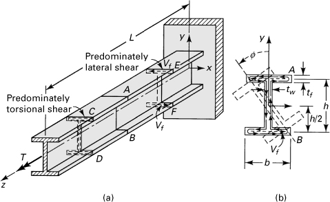
Torsional and Lateral Shears
Referring to Fig. 6.22a, the applied torque T is balanced in part by the action of torsional shearing stresses and in part by the resistance of the flanges to bending. At the representative section AB (Fig. 6.22b), consider the influence of torques T1 and T2. The former is attributable to pure torsional shearing stresses in the entire cross section, assumed to occur as though each cross section were free to warp. Torque T1 is thus related to the angle of twist of section AB by the expression
(a)
in which C is the torsional rigidity of the beam. The right-hand rule should be applied to furnish the sign convention for both torque and angle of twist. A pair of lateral shearing forces owing to bending of the flanges acting through the moment arm h gives rise to torque T2:
(b)
An expression for Vf may be derived by considering the x displacement, u. Because the beam cross section is symmetrical and the deformation small, we have u = (h/2)φ, and
(c)
Thus, the bending moment Mf and shear Vf in the flange are
(d)
(e)
where If is the moment of inertia of one flange about the y axis. Now Eq. (b) becomes
(f)
The total torque is therefore
(6.27)
Boundary Conditions
The conditions appropriate to the flange ends are
![]()
indicating that the slope and bending moment are zero at the fixed and free ends, respectively. The solution of Eq. (6.27) is, upon satisfying these conditions,
(g)
where
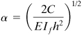
(6.28)
Long Beams
For a beam of infinite length, Eq. (g) reduces to
(h)
By substituting Eq. (h) into Eqs. (a) and (f), the following expressions result:
(6.29)
From this, it is noted that at the fixed end (z = 0) T1 = 0 and T2 = T. At this end, the applied torque is counterbalanced by the effect of shearing forces only, which from Eq. (b) are given by Vf = T2/h = T/h. The torque distribution, Eq. (6.29), indicates that sections such as EF, close to the fixed end, contain predominantly lateral shearing forces (Fig. 6.22a). Sections such as CD, near the free end, contain mainly torsional shearing stresses (as Eq. 6.29 indicates for z → ∞).
The flange bending moment, obtained from Eqs. (d) and (h), is a maximum at z = 0:
(i)
The maximum bending moment, occurring at the fixed end of the flange, is found by substituting the relations (6.28) into (i):
(6.30)
An expression for the angle of twist is determined by integrating Eq. (h) and satisfying the condition φ = 0 at z = 0:
For relatively long beams, for which e–αz may be neglected, the total angle of twist at the free end is, from Eq. (j),
(6.31)
In this equation the term 1/α indicates the influence of flange bending on the angle of twist. Since for pure torsion the total angle of twist is given by φ = TL/C, it is clear that end restraint increases the stiffness of the beam in torsion.
Example 6.9. Analysis of I-Beam Under Torsion
A cantilever I-beam with the idealized cross section shown in Fig. 6.22 is subjected to a torque of 1.2 kN · m. Determine (a) the maximum longitudinal stress, and (b) the total angle of twist, φ. Take G = 80 GPa and E = 200 GPa. Let tf = 10 mm, tw = 7 mm, b = 0.1 m, h = 0.2 m, and L = 2.4 m.
Solution
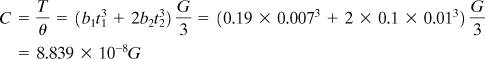
a. The torsional rigidity of the beam is, from Eq. (6.21a),
The flexural rigidity of one flange is
![]()
Hence, from Eq. (6.28) we have
![]()
From Eq. (6.30), the bending moment in the flange is found to be 3.43 times larger than the applied torque, T. Thus, the maximum longitudinal bending stress in the flange is
![]()
b. Since e–αL = 0.03, we can apply Eq. (6.31) to calculate the angle of twist at the free end:
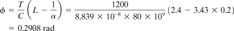
It is interesting to note that if the ends of the beam were both free, the total angle of twist would be φ = TL/C = 0.4073 rad, and the beam would experience φfree/φfixed = 1.4 times more twist under the same torque.
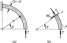
6.11 Curved Circular Bars: Helical Springs
The assumptions of Section 6.2 are also valid for a curved, circular bar, provided that the radius r of the bar is small in comparison with the radius of curvature R. When ![]() , for example, the maximum stress computed on the basis of the torsion formula, τ = Tr/J, is approximately 5% too low. On the other hand, if the diameter of the bar is large relative to the radius of curvature, the length differential of the longitudinal surface elements must be taken into consideration, and there is a stress concentration at the inner point of the bar. We are concerned here with the torsion of slender curved members for which r/R ≪ 1.
, for example, the maximum stress computed on the basis of the torsion formula, τ = Tr/J, is approximately 5% too low. On the other hand, if the diameter of the bar is large relative to the radius of curvature, the length differential of the longitudinal surface elements must be taken into consideration, and there is a stress concentration at the inner point of the bar. We are concerned here with the torsion of slender curved members for which r/R ≪ 1.
Frequently, a curved bar is subjected to loads that at any cross section produce a twisting moment as well as a bending moment. Expressions for the strain energy in torsion and bending have already been developed (Secs. 2.14 and 5.12), and application of Castigliano’s theorem (Sec. 10.4) leads readily to the displacements. Note that, in the design of springs manufactured from curved bars or wires, deflection is as important as strength. Springs are employed to apply forces or torques in a mechanism or to absorb the energy owing to suddenly applied loads.*
Consider the case of a cylindrical rod or bar bent into a quarter-circle of radius R, as shown in Fig. 6.23a. The rod is fixed at one end and loaded at the free end by a twisting moment T. The bending and twisting moments at any section are (Fig. 6.23b)
(a)
Figure 6.23. Twisting of a curved, circular bar.
Substituting these quantities into Eqs. (2.63) and (2.61) together with dx = ds = Rdθ yields
or
![]()
where J = πd4/32 = 2I. The strain energy in the entire rod is obtained by integrating:
(6.32)
Upon application of φ = ∂U/∂T, it is found that
(6.33)
for the angle of twist at the free end.
A helical spring, produced by wrapping a wire around a cylinder in such a way that the wire forms a helix of uniformly spaced turns, as typifies a curved bar, is discussed in the following example.
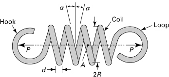
Example 6.10. Analysis of a Helical Spring
An open-coiled helical spring wound from wire of diameter d, with pitch angle α and n number of coils of radius R, is extended by an axial load P (Fig. 6.24). (a) Develop expressions for maximum stress and deflection. (b) Redo part (a) for the spring closely coiled. Assumption: Load is applied steadily at a rigid hook and loop at ends.
Figure 6.24. Example 6.10. Helical spring under tension.
Solution
An element of the spring located between two adjoining sections of the wire may be treated as a straight circular bar in torsion and bending. This is because a tangent to the coil at any point such as A is not perpendicular to the load. At cross section A, components P cos α and P sin α produce the following respective torque and moment:
(c)
a. The stresses, from Eq. (4.7), are given by
![]()
The maximum normal stress and the maximum shear stress are thus
(6.34a)
and
(6.34b)
The deflection is computed by applying Castigliano’s theorem together with Eqs. (b) and (c):
![]()
where the length of the coil L = 2πRn. It follows that the relationship
![]()
or
(6.35)
defines the axial end deflection of an open-coil helical spring.
b. For a closely coiled helical spring, the angle of pitch α of the coil is very small. The deflection is now produced entirely by the torsional stresses induced in the coil. To derive expressions for the stress and deflection, let α = sin α = 0 and cos α = 1 in Eqs. (6.34) and (6.35). In so doing, we obtain
(6.36)
and
(6.37)
Comment
The foregoing results are applicable to both tension and compression helical springs, the wire diameters of which are small in relation to coil radius.
References
6.1. UGURAL, A. C., Mechanics of Materials, Wiley, Hoboken, N. J., 2008, Sec. 6. 2.
6.2. TODHUNTER, I. and PEARSON, K., History of the Theory of Elasticity and the Strength of Materials, Dover, New York, 1960, Vols. I and II.
6.3. TIMOSHENKO, S. P., and GOODIER, J. N., Theory of Elasticity, 3rd ed., McGraw-Hill, New York, 1970.
6.4. YOUNG, W. C. and BUDYNAS, R. G., Roark’s Formulas for Stress and Strain, 6th ed., McGraw-Hill, New York, 1989.
6.5. UGURAL, A. C., Mechanical Design: An Integrated Approach, McGraw-Hill, New York, 2004, Chap. 14.
6.6. WAHL, A. M., Mechanical Springs, McGraw-Hill, New York, 1963.
Problems
Sections 6.1 through 6.3
6.1. A hollow steel shaft of outer radius c = 35 mm is fixed at one end and subjected to a torque T = 3 kN · m at the other end. Calculate the required inner radius b, knowing that the average shearing stress is limited to 100 MPa.
6.2. A solid shaft of 40-mm diameter is to be replaced by a hollow circular tube of the same material, resisting the same maximum shear stress and the same torque. Determine the outer diameter D of the tube for the case in which its wall thickness is t = D/25.
6.3. A solid shaft of diameter d and a hollow shaft of outer diameter D = 60 mm and thickness t = D/4 are to transmit the same torque at the same maximum shear stress. What is the required diameter d the shaft?
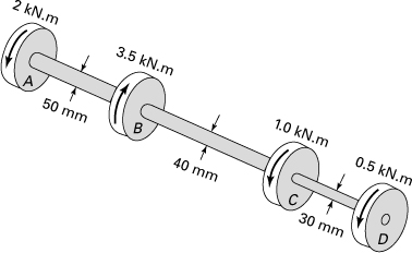
6.4. Figure P6.4 shows four pulleys, attached to a solid stepped shaft, transmit the torques. Find the maximum shear stress for each shaft segment.
6.5. Resolve Prob. 6.4, for the case in which a hole of 16-mm diameter drilled axially through the shaft to form a tube.
6.6. As seen in Fig. P6.6, a stepped shaft ABC with built-in end at A is subjected to the torques TB = 3 kN · m and TC = 1 kN · m at sections B and C. Based on a stress concentration factor K = 1.6 at the step B, what is the maximum shearing stress in the shaft? Given: d1 = 50 mm and d2 = 40 mm.
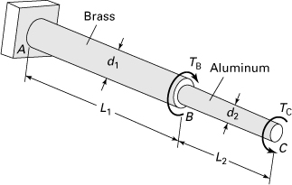
6.7. A brass rod AB (Gb = 42 GPa) is bonded to an aluminum rod BC (Gd = 28 GPa), as illustrated in Fig. P6.6. Determine the angle of twist at C, for the case in which TB = 2TC = 8 kN · m, d1 = 2d2 = 100 mm, and L1 = 2L2 = 0.7 m.
6.8. A hollow shaft is made by rolling a metal plate of thickness t into a cylindrical form and welding the edges along the helical seams oriented at an angle of φ to the axis of the member (Fig. P6.8). Calculate the maximum torque that can be applied to the shaft. Assumption: The allowable tensile and shear stresses in the weld are 120 MPa and 50 MPa, respectively. Given: D = 100 mm, t = 5 mm, and φ = 50°.
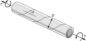
6.9. Resolve Prob. 6.8 for the case in which the helical seam is oriented at an angle of φ = 35° to the axis of the member (Fig. P6.8).
6.10. What is the required diameter d1 for the segment AB of the shaft illustrated in Fig. P6.6 if the permissible shear stress is τall = 50 MPa and the total angle of twist between A and C is limited to φ = 0.02 rad? Given: G = 39 GPa, TB = 3 kN · m, TC = 1 kN · m, L1 = 2 m, L2 = 1 m, and d2 = 25 mm.
6.11. Redo Prob. 6.10 for the case in which the torque applied at B is TB = 2 kN · m and TC = 0.5 kN · m.
6.12. A stepped shaft of diameters D and d is under a torque T, as shown in Fig. P6.12. The shaft has a fillet of radius r (see Fig. D.4). Determine (a) the maximum shear stress in the shaft for r = 1.0 mm; (b) the maximum shear stress in the shaft for r = 5 mm. Given: D = 60 mm, d = 50 mm, and T = 2 kN · m.
6.13. A stepped shaft having solid circular parts with diameters D and d is in pure torsion (Fig. P6.12). The two parts are joined with a fillet of radius r (see Fig. D.4). If the shaft is made of brass with allowable shear strength 80 MPa, determine the largest torque capacity of the shaft. Given: D = 100 mm, d = 50 mm, r = 10 mm.
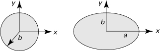
6.14. Consider two bars, one having a circular section of radius b, the other an elliptic section with semiaxes a, b (Figure P6.14). Determine (a) for equal angles of twist, which bar experiences the larger shearing stress, and (b) for equal allowable shearing stresses, which bar resists a larger torque.
6.15. A hollow (ri = b, r0 = c) and a solid (r0 = a) cylindrical shaft are constructed of the same material. The shafts are of identical length and cross-sectional area and both are subjected to pure torsion. Determine the ratio of the largest torques that may be applied to the shafts for c = 1.4b (a) if the allowable stress is τa and (b) if the allowable angle of twist is θa.
6.16. A solid circular shaft AB, held rigidly at both ends, has two different diameters (Fig. 6.4a). For a maximum permissible shearing stress τall = 150 MPa, calculate the allowable torque T that may be applied at section C. Use da = 20 mm, db = 15 mm, and a = 2b = 0.4 m.
6.17. Redo Problem 6.16 for τall = 70 MPa, da = 25 mm, db = 15 mm, and a = 1.6b = 0.8 m.
Sections 6.4 through 6.7
6.18. The stress function appropriate to a solid bar subjected to torques at its free ends is given by
Φ = k(a2 – x2 + by2)(a2 + bx2 – y2)
where a and b are constants. Determine the value of k.
6.19. Show that Eqs. (6.6) through (6.11) are not altered by a shift of the origin of x, y, z from the center of twist to any point within the cross section defined by x = a and y = b, where a and b are constants. [Hint: The displacements are now expressed as u = –θz(y – b), v = θz(x – a), and w = w(x, y).]
6.20. Rederive Eq. (6.11) for the case in which the stress function Φ = c on the boundary, where c is a nonzero constant.
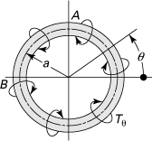
6.21. The thin circular ring of cross-sectional radius r, shown in Fig. P6.21, is subjected to a distributed torque per unit length, Tθ = Tcos2θ. Determine the angle of twist at sections A and B in terms of T, a, and r. Assume that the radius a is large enough to permit the effect of curvature on the torsion formula to be neglected.
6.22. Consider two bars of the same material, one circular of radius c, the other of rectangular section with dimensions a × 2a. Determine the radius c so that, for an applied torque, both the maximum shear stress and the angle of twist will not exceed the corresponding quantities in the rectangular bar.
6.23. The torsion solution for a cylinder of equilateral triangular section (Fig. 6.11) is derivable from the stress function, Eq. (j) of Section 6.5:
![]()
Derive expressions for the maximum and minimum shearing stresses and the twisting angle.
6.24. The torsional rigidity of a circle, an ellipse, and an equilateral triangle (Fig. 6.11) are denoted by Cc, Ce, and Ct, respectively. If the cross-sectional areas of these sections are equal, demonstrate that the following relationships exist:
![]()
where a and b are the semiaxes of the ellipse in the x and y directions.
6.25. Two thin-walled circular tubes, one having a seamless section, the other (Fig. 6.17a) a split section, are subjected to the action of identical twisting moments. Both tubes have equal outer diameter do, inner diameter di, and thickness t. Determine the ratio of their angles of twist.
6.26. A steel bar of slender rectangular cross section (5mm × 125 mm) is subjected to twisting moments of 80 N · m at the ends. Calculate the maximum shearing stress and the angle of twist per unit length. Take G = 80 GPa.
6.27. The torque T produces a rotation of 15° at free end of the steel bar shown in Fig. P6.27. Use a = 24 mm, b = 16 mm, L = 400 m, and G = 80 GPa. What is the maximum shearing stress in the bar?
6.28. Determine the largest permissible b × b square cross section of a steel shaft of length L = 3 m, for the shearing stress is not to exceed 120 MPa and the shaft is twisted through 25° (Fig. P6.27). Take G = 75 GPa.
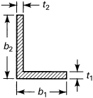
6.29. A steel bar (G = 200 GPa) of cross section as shown in Fig. P6.29 is subjected to a torque of 500 N · m. Determine the maximum shearing stress and the angle of twist per unit length. The dimensions are b1 = 100 mm, b2 = 125 mm, t1 = 10 mm, and t2 = 4 mm.
6.30. Rework Example 6.4 for the case in which segments AC and CB of torsion member AB have as a cross section an equilateral triangular of sides a1 = 60 mm and a2 = 45 mm, respectively.
6.31. Derive an approximate expression for the twisting moment in terms of G, θ, b, and to for the thin triangular section shown in Fig. P6.31. Assume that at any y the expression for the stress function Φ corresponds to a parabolic membrane appropriate to the width at that y: Φ = Gθ[(t/2)2 – x2].

6.32. Consider the following sections: (a) a hollow tube of 50-mm outside diameter and 2.5-mm wall thickness, (b) an equal-leg angle, having the same perimeter and thickness as in (a), (c) a square box section with 50-mm sides and 2.5-mm wall thickness. Compare the torsional rigidities and the maximum shearing stresses for the same applied torque.
6.33. The cross section of a 3-m-long steel bar is an equilateral triangle with 50-mm sides. The bar is subjected to end twisting couples causing a maximum shearing stress equal to two-thirds of the elastic strength in shear (τyp = 420 MPa). Using Table 6.2, determine the angle of twist between the ends. Let G = 80 GPa.
Sections 6.8 through 6.11
6.34. Show that when Eq. (6.2) is applied to a thin-walled tube, it reduces to Eq. (6.22).
6.35. A torque T is applied to a thin-walled tube of a cross section in the form of a regular hexagon of constant wall thickness t and mean side length a. Derive relationships for the shearing stress τ and the angle of twist θ per unit length.
6.36. Redo Example 6.7 with a 0.01-m-thick vertical wall at the middle of the section.
6.37. The cross section of a thin-walled aluminum tube is an equilateral triangular section of mean side length 50 mm and wall thickness 3.5 mm. If the tube is subjected to a torque of 40 N · m, what are the maximum shearing stress and angle of twist per unit length? Let G = 28 GPa.
6.38. A square thin-walled tube of mean dimensions a × a and a circular thin-walled tube of mean radius c, both of the same material, length, thickness t, and cross-sectional area, are subjected to the same torque. Determine the ratios of the shearing stresses and the angle of twist of the tubes.
6.39. A hollow, multicell aluminum tube (cross section shown in Fig. P6.39) resists a torque of 4 kN · m. The wall thicknesses are t1 = t2 = t4 = t5 = 0.5 mm and t3 = 0.75 mm. Determine the maximum shearing stresses and the angle of twist per unit length. Let G = 28 GPa.
6.40. Consider two closely coiled helical springs, one made of steel, the other of copper, each 0.01 m in wire diameter, one fitting within the other. Each has an identical number of coils, n = 20, and ends constrained to deflect the same amount. The steel outer spring has a diameter of 0.124 m, and the copper inner spring, a diameter of 0.1 m. Determine (a) the total axial load the two springs can jointly sustain if the shear stresses in the steel and the copper are not to exceed 500 and 300 MPa, respectively, and (b) the ratio of spring constants. For steel and copper, use shear moduli of elasticity Gs = 79 GPa and Gc = 41 GPa, respectively.