Chapter 8. Axisymmetrically Loaded Members
8.1 Introduction
In the class of axisymmerically loaded members, the fundamental problem may be defined in terms of the radial coordinate. There are numerous practical situations in which the distribution of stress manifests symmetry about an axis. Examples include pressure vessels, compound cylinders, clad reactor elements, chemical reaction vessels, heat exchanger tubes, solid or hollow spherical structures, turbine disks, and components of many other machines used in aerospace to household. This chapter concerns mainly “exact” stress distribution in various axisymmetrically loaded machine and structural components. The methods of mechanics of materials, the theory of elasticity, and finite elements are used. The displacements, strains, and stresses at locations far removed from the ends due to pressure, thermal, and dynamic loadings are discussed. Applications to compound press or shrink-fit cylinders, disk flywheels, and design of hydraulic cylinders are included. Before doing these, however, we begin with an analysis of stress developed in thick-walled vessels.
Basic Relations
Consider a large thin plate having a small circular hole subjected to uniform pressure, as shown in Fig. 8.1. Note that axial loading is absent, and therefore σz = 0. The stresses are clearly symmetrical about the z axis, and the deformations likewise display θ independence. The symmetry argument also dictates that the shearing stresses τrθ must be zero. Assuming z independence for this thin plate, the polar equations of equilibrium (3.31), reduce to
(8.1)
Figure 8.1. Large thin plate with a small circular hole.
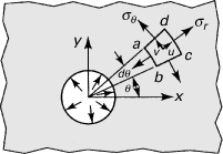
Here σθ and σr denote the tangential (circumferential) and radial stresses acting normal to the sides of the element, and Fr represents the radial body force per unit volume, for example, the inertia force associated with rotation. In the absence of body forces, Eq. (8.1) reduces to
(8.2)
Consider now the radial and tangential displacements u and v, respectively. There can be no tangential displacement in the symmetrical field; that is, v = 0. A point represented by the shaded element abcd in the figure will thus move radially as a consequence of loading, but not tangentially. On the basis of displacements indicated, the strains given by Eqs. (3.33) become
(8.3)
Substituting u = rεθ into the first expression in Eq. (8.3), a simple compatibility equation is obtained:
![]()
or
(8.4)
The equation of equilibrium [Eq. (8.1) or (8.2)], the strain–displacement or compatibility relations [Eqs. (8.3) or (8.4)], and Hooke’s law are sufficient to obtain a unique solution to any axisymmetrical problem with specified boundary conditions.
8.2 Thick-Walled Cylinders
The circular cylinder, of special importance in engineering, is usually divided into thin-walled and thick-walled classifications. A thin-walled cylinder is defined as one in which the tangential stress may, within certain prescribed limits, be regarded as constant with thickness. The following familiar expression applies to the case of a thin-walled cylinder subject to internal pressure:
![]()
Here p is the internal pressure, r the mean radius (see Sec. 13.13), and t the thickness. If the wall thickness exceeds the inner radius by more than approximately 10%, the cylinder is generally classified as thick walled, and the variation of stress with radius can no longer be disregarded (see Prob. 8.1).
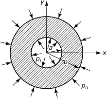
In the case of a thick-walled cylinder subject to uniform internal or external pressure, the deformation is symmetrical about the axial (z) axis. Therefore, the equilibrium and strain–displacement equations, Eqs. (8.2) and (8.3), apply to any point on a ring of unit length cut from the cylinder (Fig. 8.2). Assuming that the ends of the cylinder are open and unconstrained, σz = 0, as is subsequently demonstrated. Thus, the cylinder is in a condition of plane stress and, according to Hooke’s law (3.34), the strains are given by
(8.5)
Figure 8.2. Thick-walled cylinder.
From these, σr and σθ are as follows:
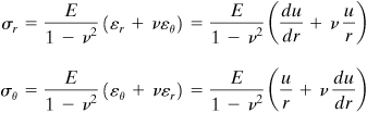
(8.6)
Substituting this into Eq. (8.2) results in the following equidimensional equation in radial displacement:
(8.7)
having a solution
(a)
The radial and tangential stresses may now be written in terms of the constants of integration c1 and c2 by combining Eqs. (a) and (8.6):
(b)
(c)
The constants are determined from consideration of the conditions pertaining to the inner and outer surfaces.
Observe that the sum of the radial and tangential stresses is constant, regardless of radial position: σr + σθ = 2Ec1/(1 – ν). Hence, the longitudinal strain is constant:
![]()
We conclude, therefore, that plane sections remain plane subsequent to loading. Then σz = Eεz = constant = c. But if the ends of the cylinder are open and free,
![]()
or c = σz = 0, as already assumed previously.
For a cylinder subjected to internal and external pressures pi and po, respectively, the boundary conditions are
(d)
where the negative sign connotes compressive stress. The constants are evaluated by substitution of Eqs. (d) into (b):
(e)
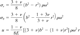
leading finally to
(8.8)
These expressions were first derived by French engineer G. Lamé in 1833, for whom they are named. The maximum numerical value of σr is found at r = a to be pi, provided that pi exceeds po. If po > pi, the maximum σr occurs at r = b and equals po. On the other hand, the maximum σθ occurs at either the inner or outer edge according to the pressure ratio, as discussed in Section 8.3.
Recall that the maximum shearing stress at any point equals one-half the algebraic difference between the maximum and minimum principal stresses. At any point in the cylinder, we may therefore state that
(8.9)
The largest value of τmax is found at r = a, the inner surface. The effect of reducing po is clearly to increase τmax. Consequently, the greatest τmax corresponds to r = a and po = 0:
(8.10)
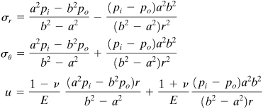
Because σr and σθ are principal stresses, τmax occurs on planes making an angle of 45° with the plane on which σr and σθ act, as depicted in Fig. 8.3. This is quickly confirmed by a Mohr’s circle construction. The pressure pyp that initiates yielding at the inner surface is obtained by setting τmax = σyp/2 in Eq. (8.10):
(8.11)
Figure 8.3. (a) Thick-walled cylinder under pi; (b) an element at the inner edge in which τmax occurs.
Here σyp is the yield stress in uniaxial tension.
Special Cases
Internal Pressure Only
If only internal pressure acts, Eqs. (8.8) reduce to
(8.12)
(8.14)
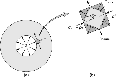
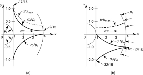
Since b2/r2 ≥ 1, σr is negative (compressive) for all r except r = b, in which case σr = 0, the maximum radial stress occurs at r = a. As for σθ, it is positive (tensile) for all radii and also has a maximum at r = a.
To illustrate the variation of stress and radial displacement for the case of zero external pressure, dimensionless stress and displacement are plotted against dimensionless radius in Fig. 8.4a for b/a = 4.
Figure 8.4. Distribution of stress and displacement in a thick-walled cylinder with b/a = 4: (a) under internal pressure; (b) under external pressure.
External Pressure Only
In this case, pi = 0, and Eq. (8.8) becomes
(8.15)
(8.16)
(8.17)
The maximum radial stress occurs at r = b and is compressive for all r. The maximum σθ is found at r = a and is likewise compressive.
For a cylinder with b/a = 4 and subjected to external pressure only, the stress and displacement variations over the wall thickness are shown in Fig. 8.4b.
Example 8.1. Analysis of a Thick-Walled Cylinder
A thick-walled cylinder with 0.3-m and 0.4-m internal and external diameters is fabricated of a material whose ultimate strength is 250 MPa. Let ν = 0.3. Determine (a) for po = 0, the maximum internal pressure to which the cylinder may be subjected without exceeding the ultimate strength, (b) for pi = 0, the maximum external pressure to which the cylinder can be subjected without exceeding the ultimate strength, and (c) the radial displacement of a point on the inner surface for case (a).
Solution
a. From Eq. (8.13), with r = a,
(8.18)
or
![]()
b. From Eq. (8.16), with r = a,
(8.19)
Then
![]()
c. Using Eq. (8.14), we obtain
![]()
Closed-Ended Cylinder
In the case of a closed-ended cylinder subjected to internal and external pressures, longitudinal or z-directed stresses exist in addition to the radial and tangential stresses. For a transverse section some distance from the ends, this stress may be assumed uniformly distributed over the wall thickness. The magnitude of σz is then determined by equating the net force acting on an end attributable to pressure loading to the internal z-directed force in the cylinder wall:
piπa2 – poπb2 = (πb2 – πa2)σz
The resulting expression for longitudinal stress, applicable only away from the ends, is
(8.20)
Clearly, here it is again assumed that the ends of the cylinder are not constrained: εz ≠ 0 (see Prob. 8.13).
8.3 Maximum Tangential Stress
An examination of Figs. 8.4a and b shows that if either internal pressure or external pressure acts alone, the maximum tangential stress occurs at the innermost fibers, r = a. This conclusion is not always valid, however, if both internal and external pressures act simultaneously. There are situations, explored next, in which the maximum tangential stress occurs at r = b [Ref. 8.1].
Consider a thick-walled cylinder, as in Fig. 8.2, subject to pi and po. Denote the ratio b/a by R, po/pi by P, and the ratio of tangential stress at the inner and outer surfaces by S. The tangential stress, given by Eqs. (8.8), is written
(a)
Hence,
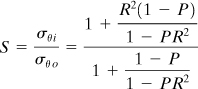
(8.21)
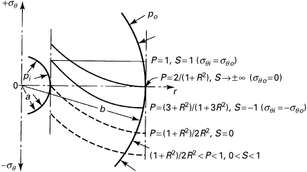
The variation of the tangential stress σθ over the wall thickness is shown in Fig. 8.5 for several values of S and P. Note that for pressure ratios P, indicated by dashed lines, the maximum magnitude of the circumferential stress occurs at the outer surface of the cylinder.
Figure 8.5. Maximum tangential stress distribution in a thick-walled cylinder under internal and external pressures.
8.4 Application of Failure Theories
Unless we are content to grossly overdesign, it is necessary to predict, as best possible, the most probable failure mechanism. Thus, while examination of Fig. 8.5 indicates that failure is likely to originate at the innermost or outermost fibers of the cylinder, it cannot predict at what pressure or stresses failure will occur. To do this, consideration must be given the stresses determined from Lamé’s equations, the material strength, and an appropriate theory of failure consistent with the nature of the material.
Example 8.2. Thick-Walled Cylinder Pressure Requirement
A steel cylinder is subjected to an internal pressure four times greater than the external pressure. The tensile elastic strength of the steel is σyp = 340 MPa, and the shearing elastic strength τyp = σyp/2 = 170 MPa. Calculate the allowable internal pressure according to the various yielding theories of failure. The dimensions are a = 0.1 m and b = 0.15 m. Let ν = 0.3.
Solution
The maximum stresses occur at the innermost fibers. From Eqs. (8.8), for r = a and pi = 4po, we have
(a)
The value of internal pressure at which yielding begins is predicted according to the various theories of failure, as follows:
a. Maximum shearing stress theory:
![]()
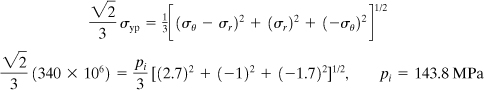
b. Energy of distortion theory [Eq. (4.5a)]:
![]()
c. Octahedral shearing stress theory: By use of Eqs. (4.6) and (1.38), we have
Comment
The results found in (b) and (c) are identical as expected (Sec. 4.8). The onset of inelastic action is governed by the maximum shearing stress: the allowable value of internal pressure is limited to 125.9 MPa, modified by an appropriate factor of safety.
8.5 Compound Cylinders: Press or Shrink Fits
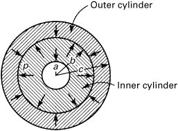
If properly designed, a system of multiple cylinders resists relatively large pressures more efficiently, that is, requires less material, than a single cylinder. To assure the integrity of the compound cylinder, one of several methods of prestressing is employed. For example, the inner radius of the outer member or jacket may be made smaller than the outer radius of the inner cylinder. The cylinders are assembled after the outer cylinder is heated, contact being effected upon cooling. The magnitude of the resulting contact pressure p, or interface pressure, between members may be calculated by use of the equations of Section 8.2. Examples of compound cylinders, carrying very high pressures, are seen in compressors, extrusion presses, and the like.
Referring to Fig. 8.6, assume the external radius of the inner cylinder to be larger, in its unstressed state, than the internal radius of the jacket, by an amount δ. The quantity δ is called the shrinking allowance, or also known as the radial interference. Subsequent to assembly, the contact pressure, acting equally on both members, causes the sum of the increase in the inner radius of the jacket and decrease in the outer radius of the inner member to exactly equal δ. By using Eqs. (8.14) and (8.17), we obtain
(8.22)
Figure 8.6. Compound cylinder.
Here Eo, νo and Ei, νi represent the material properties of the outer and inner cylinders, respectively. When both cylinders are made of the same materials, we have Eo = Ei = E and νo = νi = ν. In such a case, from Eq. (8.22),
(8.23)
The stresses in the jacket are then determined from Eqs. (8.12) and (8.13) by treating the contact pressure as pi. Similarly, by regarding the contact pressure as po, the stresses in the inner cylinder are calculated from Eqs. (8.15) and (8.16).
Example 8.3. Stresses in a Compound Cylinder under Internal Pressure
A compound cylinder with a = 150 mm, b = 200 mm, c = 250 mm, E = 200 GPa, and δ = 0.1 mm is subjected to an internal pressure of 140 MPa. Determine the distribution of tangential stress throughout the composite wall.
Solution
In the absence of applied internal pressure, the contact pressure is, from Eq. (8.23),
![]()
The tangential stresses in the outer cylinder associated with this pressure are found by using Eq. (8.13)
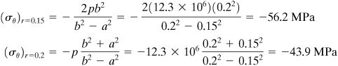
The stresses in the inner cylinder are, from Eq. (8.16),
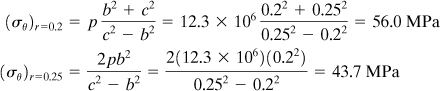
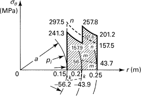
These stresses are plotted in Fig. 8.7, indicated by the dashed lines kk and mm. The stresses owing to internal pressure alone, through the use of Eq. (8.13) with b = c, are found to be (σθ)r = 0.15 = 297.5 MPa, (σθ)r = 0.2 = 201.8 MPa, (σθ)r = 0.25 = 157.5 MPa, and are shown as the dashed line nn. The stress resultant is obtained by superposition of the two distributions, represented by the solid line. The use of a compound prestressed cylinder has thus reduced the maximum stress from 297.5 to 257.8 MPa. Based on the maximum principal stress theory of elastic failure, significant weight savings can apparently be effected through such configurations.
Figure 8.7. Example 8.3. Tangential stress distribution produced by a combination of shrink-fit and internal pressure in a thick-walled compound cylinder. Dashed lines nn represent stresses due to pi alone.
It is interesting to note that additional jackets prove not as effective, in that regard, as the first one. Multilayered shrink-fit cylinders, each of small wall thickness, are, however, considerably stronger than a single jacket of the same total thickness. These assemblies can, in fact, be designed so that prestressing owing to shrinking combines with stresses due to loading to produce a nearly uniform distribution of stress throughout.* The closer this uniform stress is to the allowable stress for the given material, the more efficiently is the material utilized. A single cylinder cannot be uniformly stressed and consequently must be stressed considerably below its allowable value, contributing to inefficient use of material.
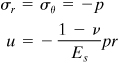
Example 8.4. Design of a Duplex Hydraulic Conduit
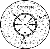
Figure 8.8 shows a duplex hydraulic conduit composed of a thin steel cylindrical liner in a concrete pipe. For the steel and concrete, the properties are Es and Ec, νc, respectively. The conduit is subjected to an internal pressure pi. Determine the interface pressure p transmitted to the concrete shell.
Figure 8.8. Example 8.4. Thick-walled concrete pipe with a steel cylindrical liner.
Solution
The radial displacement at the bore (r = a) of the concrete pipe is, from Eq. (8.14),
(a)
The steel sleeve experiences an internal pressure pi and an external pressure p. Thus,
(b)
On the other hand, Hooke’s law together with Eq. (8.2) yields at r = a
(c)
Finally, evaluation of u from Eqs. (b) and (c) and substitution into Eq. (a) result in the interface pressure in the form:
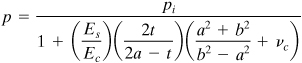
(8.24)
Comment
Note that, for practical purposes, we can use Es/Ec = 15, νc = 0.2, and 2t/(2a – t) = t/a. Equation (8.24) then becomes
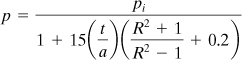
(8.25)
where R = b/a. From the foregoing, observe that, as the thickness t of the liner increases, the pressure p transmitted to the concrete decreases. However, for any given t/a ratio, the p increases as the diameter ratio (R) of the concrete increases.
8.6 Rotating Disks of Constant Thickness
The equation of equilibrium, Eq. (8.1), can be used to treat the case of a rotating disk, provided that the centrifugal “inertia force” is included as a body force. Again, stresses induced by rotation are distributed symmetrically about the axis of rotation and assumed independent of disk thickness. Thus, application of Eq. (8.1), with the body force per unit volume Fr equated to the centrifugal force ρω2r, yields
(8.26)
where ρ is the mass density and ω the constant angular speed of the disk in radians per second. Note that the gravitational body force ρg has been neglected. Substituting Eq. (8.6) into Eq. (8.26), we have
(a)
requiring a homogeneous and particular solution. The former is given by Eq. (a) of Section 8.2.
It is easily demonstrated that the particular solution is
![]()
The complete solution is therefore
(8.27a)
which, upon substitution into Eq. (8.6), provides the following expressions for radial and tangential stress:
(8.27b)
The constants of integration may now be evaluated on the basis of the boundary conditions.
Annular Disk
In the case of an annular disk with zero pressure at the inner (r = a) and outer (r = b) boundaries (Fig. 8.9) the distribution of stress is due entirely to rotational effects. The boundary conditions are
(b)
Figure 8.9. Annular rotating disk of constant thickness.
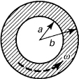
These conditions, combined with Eq. (8.27b), yield two equations in the two unknown constants,
(c)
from which
(d)
The stresses and displacement are therefore
(8.28 a–c)
Applying the condition dσr/dr = 0 to the first of these equations, it is readily verified that the maximum radial stress occurs at ![]() . Then, substituting the foregoing into Eq. (8.28a), the maximum radial stress is given by
. Then, substituting the foregoing into Eq. (8.28a), the maximum radial stress is given by
(8.29)
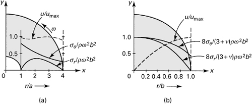
Figure 8.10a is a dimensionless representation of stress and displacement as a function of radius for an annular disk described by b/a = 4.
Figure 8.10. Distribution of stress and displacement in a rotating disk of constant thickness: (a) annular disk; (b) solid disk.
Solid Disk
In this case, a = 0, and the boundary conditions are
(e)
To satisfy the condition on the displacement, it is clear from Eq. (8.27a) that c2 must be zero. The remaining constant is now evaluated from the first expression of Eq. (d):
![]()
Combining these constants with Eqs. (8.27), the following results are obtained:
(8.30 a–c)
The stress and displacement of a solid rotating disk are displayed in a dimensionless representation (Fig. 8.10b) as functions of radial location.
The constant thickness disks discussed in this section are generally employed when stresses or speeds are low and, as is clearly shown in Fig. 8.10b, do not make optimum use of material. Other types of rotating disks, offering many advantages over flat disks, are discussed in the sections to follow.
Clearly, the sharp rise of the tangential stress near r = a is observed in Fig. 8.10a. It can be shown that, by setting r = a in Eq. (8.29b) and letting a approach zero, the resulting σθ is twice that given by Eq. (8.30b). The foregoing conclusion applies to the radial stress as well. Thus, a small hole doubles the stress over the case of no hole.
8.7 Design of Disk Flywheels
A flywheel is usually employed to smooth out changes in the speed of a shaft caused by torque fluctuations (Fig. 8.11). Flywheels are thus found in small and large machinery, such as compressors, internal combustion engines, punch presses, and rock crushers. At high speeds, considerable stresses may be induced in these components. Since failure of a rotating disk is particularly hazardous, analysis of the stress effects is important. Designing of energy-storing flywheels for hybrid-electric cars is an active area of contemporary research. Disk flywheels, that is, rotating annular disks of constant thickness, are made of high-strength steel plate.
Figure 8.11. A flywheel shrunk onto a shaft.
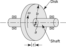
An interference fit produces stress concentration in the shaft and in the (hub of) the disk, owing to the abrupt change from uncompressed to compressed material. Various design modifications are usually made in the faces of the disk close to the shaft diameter to decrease the stress concentrations at each sharp corner. Often, for a press or shrink fit, a stress concentration factor K is used. The value of K, depending on the contact pressure, the design of the disk, and the maximum bending stress in the shaft, rarely exceeds 2 [Ref. 8.3]. It should be noted that an approximation of the torque capacity of the assembly may be made on the basis of a coefficient of friction of about f = 0.15 between shaft and disk. The American Gear and Manufacturing Association (AGMA) standard suggests a value of 0.15 < f < 0.20 for shrink or press fits having a smooth finish on both surfaces.
The Method of Superposition
Combined radial stress, tangential stress, and displacement of an annular disk due to internal pressure p between the disk and the shaft and angular speed ω may readily be obtained through the use of superposition of the results obtained previously. Therefore, we have
(8.31a)
(8.31b)
(8.31c)
In the foregoing, the quantities (σr)p, (σθ)p, and (u)p are given by Eqs. (8.8). The tangential stress σθ often controls the design. It is a maximum at the inner boundary (r = a). Hence,
(8.32)
As noted previously, owing to rotation alone, maximum radial stress occurs at ![]() and is given by Eq. (8.29). On the other hand, due to the internal pressure only, the largest radial stress is at the inner boundary and equals σr,max = –p.
and is given by Eq. (8.29). On the other hand, due to the internal pressure only, the largest radial stress is at the inner boundary and equals σr,max = –p.
It is customary to neglect the inertial stress and displacement of a shaft. Hence, for a shaft, we approximately have
(8.33)
We note, however, that the contact pressure p depends on angular speed ω. For a prescribed contact pressure p at angular speed ω, the required initial radial interference δ may be found from Eqs. (8.31c) and (8.33) for the displacement u. In so doing, with r = a, we obtain
(8.34)
Here the quantities Ed and Es represent the moduli of elasticity of the disk and shaft, respectively. Clearly, the preceding equation is valid as long as a positive contact pressure is maintained.
Example 8.5. Torque and Power Capacity of a Flywheel
A flat steel disk with t = 20 mm and a = 50 mm is shrunk onto a shaft, causing a contact pressure p (Fig. 8.11). The coefficient of static friction is f = 0.15. Determine the torque T carried by the fit and power P transmitted to the disk when the assembly is rotating at n = 2400 rpm and p = 25 Mpa.
Solution
The force (axial or tangential) required for the assembly may be written in the form
(8.35a)
The torque capacity of the fit is therefore
(8.35b)
Substituting the given numerical values,
T = 2π(502)(0.15)(25)(0.02) = 1.178 kN · m
Power transmitted is expressed by
(8.35c)
Here the angular velocity of the disk ω = 24000(2π)/60 = 251.3 rad/s. We thus have P = (1.178) (251.3) = 296 kW.
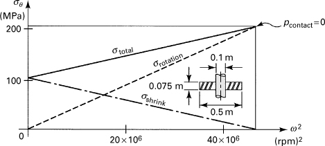
Example 8.6. Rotating Shrink-Fit Performance Analysis
A flat 0.5-m outer diameter, 0.1-m inner diameter, and 0.075-m-thick steel disk is shrunk onto a steel shaft (Fig. 8.12). If the assembly is to run at speeds up to n = 6900 rpm, determine (a) the shrinking allowance, (b) the maximum stress when not rotating, and (c) the maximum stress when rotating. The material properties are ρ = 7.8 kN · s2/m4, E = 200 GPa, and ν = 0.3.
Figure 8.12. Example 8.6. Tangential stresses produced by the combination of a shrink fit and rotation in a disk of constant thickness.
Solution
a. The radial displacements of the disk (ud) and shaft (us) are, from Eqs. (8.28) and (8.30),
We observe that us may be neglected, as it is less than 1% of ud of the disk at the common radius. The exact allowance is
b. Applying Eq. (8.23), we have
![]()
Therefore, from Eq. (8.18),
![]()
c. From Eq. (8.28), for r = 0.05,
A plot of the variation of stress in the rotating disk is shown in Fig. 8.12.
Example 8.7. Maximum Speed of a Flywheel Assembly
A flywheel of 380-mm diameter is to be shrunk onto a 60-mm diameter shaft (Fig. 8.11). Both members are made of steel with ρ = 7.8 kN · s2/m4, E = 200 GPa, and ν = 0.3. At a maximum speed of n = 6000 rpm, a contact pressure of p = 20 MPa is to be maintained. Find (a) the required radial interference; (b) the maximum tangential stress in the assembly; (c) the speed at which the fit loosens, that is, contact pressure becomes zero.
a. Through the use of Eq. (8.34), we obtain
(a)
Substituting the given numerical values p = 20 MPa and ω = 6000(2π/60) = 628.32 rad/s, Eq. (a) results in δ = 0.02 mm.
b. Applying Eq. (8.32), we obtain
c. Carrying δ = 0.02 × 10⁻³ m and p = 0 into Eq. (a) leads to
![]()
We thus have ![]() . Note that, at this speed, the shrink fit becomes completely ineffective.
. Note that, at this speed, the shrink fit becomes completely ineffective.
8.8 Rotating Disks of Variable Thickness
In Section 8.6, the maximum stress in a flat rotating disk was observed to occur at the innermost fibers. This explains the general shape of many disks: thick near the hub, tapering down in thickness toward the periphery, as in a steam turbine. This not only has the effect of reducing weight but also results in lower rotational inertia.
The approach employed in the analysis of flat disks can be extended to variable thickness disks. Let the profile of a radial section be represented by the general hyperbola (Fig. 8.13),
(8.36)
Figure 8.13. Disk of hyperbolic profile.
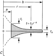
where t1 represents a constant and s a positive number. The shape of the curve depends on the value selected for s; for example, for s = 1, the profile is that of an equilateral hyperbola. The constant t1 is simply the thickness at radius equal to unity. If the thickness at r = a is ti and that at r = b is to, as shown in the figure, the hyperbolic curve is fitted by forming the ratio
![]()
and solving for s. Clearly, Eq. (8.36) does not apply to solid disks, as all values of s except zero yield infinite thickness at r = 0.
In a turbine application, the actual configuration may have a thickened outer rim to which blades are affixed and a hub for attachment to a shaft. The hyperbolic relationship cannot describe such a situation exactly, but sometimes serves as an adequate approximation. If greater accuracy is required, the hub and outer ring may be approximated as flat disks, with the elements of the assembly related by the appropriate boundary conditions.
The differential equation of equilibrium (Eq. 8.26) must now include t(r) and takes the form
(8.37)
Equation (8.37) is satisfied by a stress function of the form
(a)
Then the compatibility equation (8.4), using Eqs. (a) and Hooke’s law, becomes
(b)
Introducing Eq. (8.36), we have
(c)
This is an equidimensional equation, which the transformation r = eα reduces to a linear differential equation with constant coefficients:
(d)
The auxiliary equation corresponding to Eq. (d) is given by
m2 + sm – (1 + νs) = 0
and has the roots
(8.38)
The general solution of Eq. (d) is then
(e)
The stress components for a disk of variable thickness are therefore, from Eqs. (a),
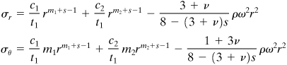
(8.39)
Note that, for a flat disk, t = constant; consequently, s = 0 in Eq. (8.36) and m = 1 in Eq. (8.38). Thus, Eqs. (8.39) reduce to Eqs. (8.30), as expected. The constants c1 and c2 are determined from the boundary conditions
(f)
The evaluation of the constants is illustrated in the next example.
Example 8.8. Rotating Hyperbolic Disk
The cross section of the disk in the assembly given in Example 8.6 is hyperbolic with ti = 0.075 m and to = 0.015 m; a = 0.05 m, b = 0.25 m, and δ = 0.05 mm. The rotational speed is 6900 rpm. Determine (a) the maximum stress owing to rotation and (b) the maximum radial displacement at the bore of the disk.
Solution
a. The value of the positive number s is obtained by the use of Eq. (8.36):
![]()
Substituting ti/to = 5 and b/a = 5, we obtain s = 1. The profile will thus be given by t = ti/r. From Eq. (8.38), we have
![]()
Hence the radial stresses, using Eqs. (8.39) and (f) for r = 0.05 and 0.25, are
from which
![]()
The stress components in the disk, substituting these values into Eqs. (8.39), are therefore
(g)
The maximum stress occurs at the bore of the disk and from Eqs. (g) is equal to (σθ)r = 0.05 = 0.0294 ρω2. Note that it was 0.052 ρω2 in Example 8.6. For the same speed, we conclude that the maximum stress is reduced considerably by tapering the disk.
b. The radial displacement is obtained from the second equation of (8.5), which together with Eq. (g) gives ur = 0.05 = (rσθ/E)r = 0.05 = 0.00147ρω2/E. Again, this is advantageous relative to the value of 0.0026 ρω2/E found in Example 8.6.
8.9 Rotating Disks of Uniform Stress
If every element of a rotating disk is stressed to a prescribed allowable value, presumed constant throughout, the disk material will clearly be used in the most efficient manner. For a given material, such a design is of minimum mass, offering the distinct advantage of reduced inertia loading as well as lower weight. What is sought, then, is a thickness variation t(r) such that σr = σθ = σ = constant everywhere in the body. Under such a condition of stress, the strains, according to Hooke’s law, are εr = εθ = ε = constant, and the compatibility equation (8.4) is satisfied.
The equation of equilibrium (8.37) may, under the conditions outlined, be written
![]()
(8.40)
which is easily integrated to yield
(8.41)
This variation assures that σθ = σr = σ = constant throughout the disk. To obtain the value of the constant in Eq. (8.41), the boundary condition t = t1 at r = 0 is applied, resulting in c1 = t1 (Fig. 8.14).
Figure 8.14. Profile of disk of uniform strength.
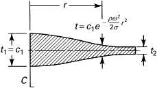
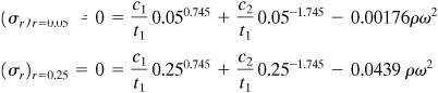
Example 8.9. Rotating Disk of Uniform Strength
A steel disk of the same outer radius, b = 0.25 m, and rotational speed, 6900 rpm, as the disk of Example 8.6 is to be designed for uniform stress. The thicknesses are t1 = 0.075 m at the center and t2 = 0.015 m at the periphery. Determine the stress and disk profile.
Solution
From Eq. (8.41),
![]()
or
![]()
Thus,
t = c1e–ρ(ω2/2σ)r2 = 0.075e–25.752r2
Recall that the maximum stress in the hyperbolic disk of Example 8.8 was 0.0294 ρω2. The uniformly stressed disk is thus about 34% stronger than a hyperbolic disk with a small hole at its center.
In actual practice, fabrication and design constraints make it impractical to produce a section of exactly constant stress in a solid disk. On the other hand, in an annular disk, if the boundary condition is applied such that the radial stress is zero at the inner radius, constancy of stress dictates that σθ and σr be zero everywhere. This is clearly not a useful result for the situation as described. For these reasons, the hyperbolic variation in thickness is often used.
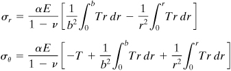
8.10 Thermal Stresses in Thin Disks
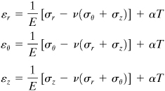
In this section, our concern is with the stresses associated with a radial temperature field T(r) that is independent of the axial dimension. The practical applications are numerous and include annular fins and turbine disks. Because the temperature field is symmetrical with respect to a central axis, it is valid to assume that the stresses and displacements are distributed in the same way as those of Section 8.1, and therefore the equations of that section apply here as well.
In this case of plane stress, the applicable equations of stress and strain are obtained from Eq. (3.37) with reference to Eq. (3.26):
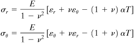
(8.42)
The equation of equilibrium, Eq. (8.2), is now
(a)
Introduction of Eq. (8.3) into expression (a) yields the following differential equation in radial displacement:
(b)
This is rewritten
(c)
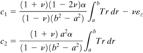
to render it easily integrable. The solution is
(8.43)
where a, the inner radius of an annular disk, is taken as zero for a solid disk, and ν and α have been treated as constants.
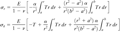
Annular Disk
The radial and tangential stresses in the annular disk of inner radius a and an outer radius b may be found by substituting Eq. (8.43) into Eq. (8.3) and the results into Eq. (8.42):
(d)
(e)
The constants c1 and cs are determined on the basis of the boundary conditions (σr)r = a = (σr)r = b = 0. Equation (d) thus gives
![]()
The stresses are therefore
(8.44)
Solid Disk
In the case of a solid disk of radius b, the displacement must vanish at r = 0 in order to preserve the continuity of material. The value of c2 in Eq. (8.43) must therefore be zero. To evaluate c1, the boundary condition (σr)r=b = 0 is employed, and Eq. (d) now gives
![]()
Substituting c1 and c2 into Eqs. (d) and (e), the stresses in a solid disk are found to be
(8.45)
Given a temperature distribution T(r), the stresses in a solid or annular disk can thus be determined from Eqs. (8.44) or (8.45). Note that T(r) need not be limited to those functions that can be analytically integrated. A numerical integration can easily be carried out for σr, σθ to provide results of acceptable accuracy.
8.11 Thermal Stress in Long Circular Cylinders
Consider a long cylinder with ends assumed restrained so that w = 0. This is another example of plane strain, for which εz = 0. The stress–strain relations are, from Hooke’s law,
(8.46)
For εz = 0, the final expression yields
(a)
Substitution of Eq. (a) into the first two of Eqs. (8.46) leads to the following forms in which z stress does not appear:
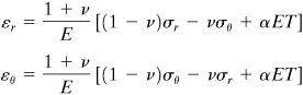
(8.47)
Inasmuch as Eqs. (8.2) and (8.3) are valid for the case under discussion, the solutions for u, σr, and σθ proceed as in Section 8.10, resulting in
(b)
(c)
(d)
Finally, from Eq. (a), we obtain
(e)
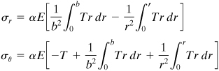
Solid Cylinder
For the radial displacement of a solid cylinder of radius b to vanish at r = 0, the constant c2 in Eq. (b) must clearly be zero. Applying the boundary condition (σr)r = b = 0, Eq. (c) may be solved for the remaining constant of integration,
(f)
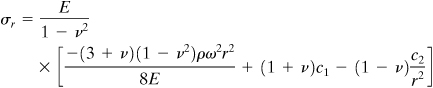
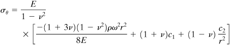
and the stress distributions determined from Eqs. (c), (d), and (e):
(8.48)
(8.49a)
To derive an expression for the radial displacement, c2 = 0 and Eq. (f) are introduced into Eq. (b).
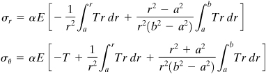
The longitudinal stress given by Eq. (8.49a) is valid only for the case of a fixed-ended cylinder. In the event the ends are free, a uniform axial stress σz = s0 may be superimposed to cause the force resultant at each end to vanish:
![]()
This expression together with Eq. (e) yields
(g)
The longitudinal stress for a free-ended cylinder is now obtained by adding s0 to the stress given by Eq. (e):
(8-49b)
Stress components σr and σθ remain as before. The axial displacement is obtained by adding u0 = –νs0r/E, a displacement due to uniform axial stress, s0, to the right side of Eq. (b).
Cylinder with Central Circular Hole
When the inner (r = a) and outer (r = b) surfaces of a hollow cylinder are free of applied load, the boundary conditions (σr)r = a = (σr)r = b = 0 apply. Introducing these into Eq. (c), the constants of integration are
(h)
Equations (c), (d), and (e) thus provide
(8.50)
(8.51a)
If the ends are free, proceeding as in the case of a solid cylinder, the longitudinal stress is described by
(8.51b)
Implementation of the foregoing analyses depends on a knowledge of the radial distribution of temperature T(r).
Example 8.10. Thermal Stresses in a Cylinder
Determine the stress distribution in a hollow free-ended cylinder, subject to constant temperatures Ta and Tb at the inner and outer surfaces, respectively.
Solution
The radial steady-state heat flow through an arbitrary internal cylindrical surface is given by Fourier’s law of conduction:
(i)
Here Q is the heat flow per unit axial length and K the thermal conductivity. Assuming Q and K to be constant,
![]()
This is easily integrated upon separation:
(j)
Here c1 and c2, the constants of integration, are determined by applying the temperature boundary conditions (T)r = a = Ta and (T)r = b = Tb. By so doing, Eq. (j) may be written in the form
(8.52)
When this is substituted into Eqs. (8.50) and (8.51a), the following stresses are obtained:
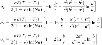
(8.53)
We note that, for ν = 0, Eqs. (8.53) provide a solution for a thin hollow disk. In the event the heat flow is outward, that is, Ta > Tb, examination of Eqs. (8.53) indicates that the stresses σθ and σz are compressive (negative) on the inner surface and tensile (positive) on the outer surface. They exhibit their maximum values at the inner and outer surfaces. On the other hand, the radial stress is compressive at all points and becomes zero at the inner and outer surfaces of the cylinder.
In practice, a pressure loading is often superimposed on the thermal stresses, as in the case of chemical reaction vessels. An approach is to follow similarly to that already discussed, with boundary conditions modified to reflect the pressure; for example, (σr)r = a = –pi, (σr)r = b = 0. In this instance, the internal pressure results in a circumferential tensile stress (Fig. 8.4a), causing a partial cancellation of compressive stress owing to temperature.
Note that, when a rotating disk is subjected to inertia, loading combined with an axisymmetrical distribution of temperature T(r), the stresses and displacements may be determined by superposition of the two cases.
8.12 Finite Element Solution
In the previous sections, the cases of axisymmetry discussed were ones in which along the axis of revolution (z) there was uniformity of structural geometry and loading. In this section, the finite element approach of Chapter 7 is applied for computation of displacement, strain, and stress in a general axisymmetric structural system, formed as a solid of revolution having material properties, support conditions, and loading, all of which are symmetrical about the z axis, but that may vary along this axis. A simple illustration of this situation is a sphere uniformly loaded by gravity forces.
“Elements” of the body of revolution (rings or, more generally, tori) are used to discretize the axisymmetric structure. We shall here employ an element of triangular cross section, as shown in Fig. 8.15. Note that a node is now in fact a circle; for example, node i is the circle with ri as radius. Thus, the elemental volume dV appearing in the expressions of Section 7.13 is the volume of the ring element (2πr dr dz).
Figure 8.15. Triangular cross section of axisymmetric solid finite element.
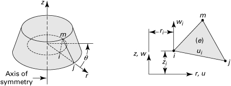
The element clearly lies in three-dimensional space. Any randomly selected vertical cross section of the element, however, is a plane triangle. As already discussed in Section 8.1, no tangential displacement can exist in the symmetrical system; that is, v = 0. Inasmuch as only the radial displacement u and the axial displacement w in a plane are involved (rz plane), the expressions for displacement established for plane stress and plane strain may readily be extended to the axisymmetric analysis [Ref. 8.4].
8.13 Axisymmetric Element
The theoretical development follows essentially the procedure given in Chapter 7, with the exception that, in the present case, cylindrical coordinates are employed (r, θ, z), as shown in Fig. 8.15.
Strain, Stress, and Elasticity Matrices
The strain matrix, from Eqs. (2.4), (3.33a), and (3.33b), may be defined as follows:
(8.54)
The initial strain owing to a temperature change is expressed in the form
{ε0}e = {αT, αT, αT, 0}
It is observed from Eq. (8.54) that the tangential strain εθ becomes infinite for a zero value of r. Thus, if the structural geometry is continuous at the z axis, as in the case of a solid sphere, r is generally assigned a small value (for example, 0.1 mm) for the node located at this axis.
It can be demonstrated that the state of stress throughout the element {σ}e is expressible as follows:
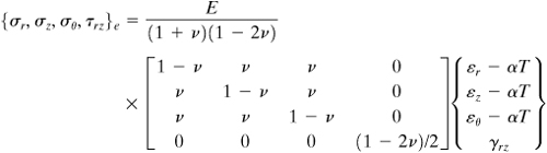
(8.55)
A comparison of Eqs. (8.55) and (7.58) yields the elasticity matrix
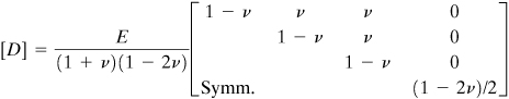
(8.56)
Displacement Function
The nodal displacements of the element are written in terms of submatrices δu and δv:
(a)
The displacement function {f}e, which describes the behavior of the element, is given by
(8.57a)
or
(8.57b)
Here the α’s are the constants, which can be evaluated as follows. First, we express the nodal displacements {δ}e:
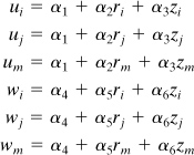
Then, by the inversion of these linear equations,
(8.58)
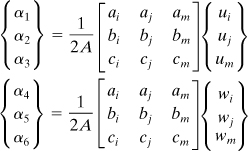
where A is defined by Eq. (7.67) and
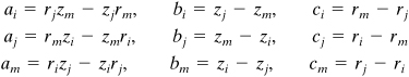
(8.59)
Finally, upon substitution of Eqs. (8.58) into (8.57), the displacement function is represented in the following convenient form:
(8.60)
or
{f}e = [N]{δ}e
with
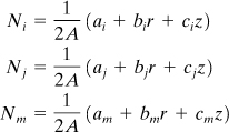
(8.61)
The element strain matrix is found by introducing Eq. (8.60) together with (8.61) into (8.54):
(8.62)
where
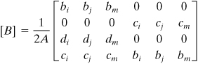
(8.63)
with
![]()
It is observed that the matrix [B] includes the coordinates r and z. Thus, the strains are not constant, as is the case with plane stress and plane strain.
The Stiffness Matrix
The element stiffness matrix, from Eq. (7.61), is given by
(8.64a)
and must be integrated along the circumferential or ring boundary. This may thus be rewritten
where the matrices [D] and [B] are defined by Eqs. (8.56) and (8.63), respectively. It is observed that integration is not easily performed as in the case of plane stress problems, because [B] is also a function of r and z. Although tedious, the integration can be carried out explicitly. Alternatively, approximate numerical approaches may be used. In a simple approximate procedure, [B] is evaluated for a centroidal point of the element. To accomplish this, we substitute fixed centroidal coordinates of the element
(8.65)
into Eq. (8.63) in place of r and z to obtain ![]() . Then, by letting
. Then, by letting ![]() , from Eqs. (8.64), the element stiffness is found to be
, from Eqs. (8.64), the element stiffness is found to be
(8.66)
This simple procedure leads to results of acceptable accuracy.
External Nodal Forces
In the axisymmetric case, “concentrated” or “nodal” forces are actually loads axisymmetrically located around the body. Let qr and qz represent the radial and axial components of force per unit length, respectively, of the circumferential boundary of a node or a radius r. The total nodal force in the radial direction is
(8.67a)
Similarly, the total nodal force in the axial direction is
(8.67b)
Other external load components can be treated analogously. When the approximation leading to Eq. (8.66) is used, we can, from Eq. (7.58), readily obtain expressions for nodal forces owing to the initial strains, body forces, and any surface tractions (see Prob. 8.49).
In summary, the solution of an axisymmetric problem can be obtained, having generated the total stiffness matrix [K], from Eq. (8.64) or (8.66), and the load matrices {Q}. Then Eq. (7.60) provides the numerical values of nodal displacements {δ} = [K]–1{Q}. The expression (8.62) together with Eq. (8.63) yields values of the element strains. Finally, Eq. (8.55), upon substitution of Eq. (8.62), is used to determine the element stresses.
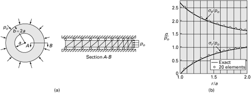
Case Study 8.1 Thick-Walled High-Pressure Steel Cylinder
Figure 8.16. Case Study 8.1. (a) Thick-walled cylinder subjected to external pressure and modeling of a slice at section A–B; (b) distribution of tangential and radial stresses in the cylinder for b = 2a.
Solution
References
8.1. RANOV, T. and PARK, F. R., On the numerical value of the tangential stress on thick-walled cylinders, J. Appl. Mech., March 1953.
8.2. BECKER, S. J. and MOLLICK, L., The theory of the ideal design of a compound vessel, Trans. ASME, J. Engineering Industry, May 1960, 136.
8.3. UGURAL, A. C., Mechanical Design: An Integrated Approach, McGraw-Hill, New York, 2004, Chap. 16.
8.4. YANG, T. Y., Finite Element Structural Analysis, Prentice Hall, Englewood Cliffs, N.J., 1986, Chap. 10.
8.5. ZIENKIEWICZ, O. C. and TAYLOR, R. I., The Finite Element Method, 4th ed., Vol. 2 (Solid and Fluid Mechanics, Dynamics and Nonlinearity), McGraw-Hill, London, 1991.
8.6. COOK, R. D., Concepts and Applications of Finite Element Analysis, 2nd ed., Wiley, New York, 1980.
8.7. BATHE, K. I., Finite Element Procedures in Engineering Analysis, Prentice Hall, Upper Saddle River, N.J., 1996.
8.8. DUNHAM, R. S. and NICKELL, R. E., “Finite element analysis of axisymmetric solids with arbitrary loadings,” Report AD 655 253, National Technical Information Service, Springfield, VA, June 1967.
8.9. UTKU, S., Explicit expressions for triangular torus element stiffness matrix, AIAA Journal, 6/6, 1174–1176, June 1968.
Problems
Sections 8.1 through 8.5
8.1. A cylinder of internal radius a and external radius b = 1.10a is subjected to (a) internal pressure pi only and (b) external pressure po only. Determine for each case the ratio of maximum to minimum tangential stress.
8.2. A thick-walled cylinder with closed ends is subjected to internal pressure pi only. Knowing that a = 0.6 m, b = 1 m, σall = 140 MPa, and τall = 80 MPa, determine the allowable value of pi.
8.3. A cylinder of inner radius a and outer radius na, where n is an integer, has been designed to resist a specific internal pressure, but reboring becomes necessary. (a) Find the new inner radius rx required so that the maximum tangential stress does not exceed the previous value by more than Δσθ, while the internal pressure is the same as before. (b) If a = 25 mm and n = 2 and after reboring the tangential stress is increased by 10%, determine the new diameter.
8.4. A steel tank having an internal diameter of 1.2 m is subjected to an internal pressure of 7 MPa. The tensile and compressive elastic strengths of the material are 280 MPa. Assuming a factor of safety of 2, determine the wall thickness.
8.5. Two thick-walled, closed-ended cylinders of the same dimensions are subjected to internal and external pressure, respectively. The outer diameter of each is twice the inner diameter. What is the ratio of the pressures for the following cases? (a) The maximum tangential stress has the same absolute value in each cylinder. (b) The maximum tangential strain has the same absolute value in each cylinder. Take ![]() .
.
8.6. Determine the radial displacement of a point on the inner surface of the tank described in Prob. 8.4. Assume that outer diameter 2b = 1.2616 m, E = 200 GPa, and ν = 0.3.
8.7. Derive expressions for the maximum circumferential strains of a thick-walled cylinder subject to internal pressure pi only, for two cases: (a) an open-ended cylinder and (b) a closed-ended cylinder. Then, assuming that the allowable strain is limited to 1000 μ, pi = 60 MPa, and b = 2 m, determine the required wall thickness. Use E = 200 GPa and ![]() .
.
8.8. An aluminum cylinder (E = 72 GPa, ν = 0.3) with closed and free ends has a 500-mm external diameter and a 100-mm internal diameter. Determine maximum tangential, radial, shearing, and longitudinal stresses and the change in the internal diameter at a section away from the ends for an internal pressure of pi = 60 MPa.
8.9. Rework Prob. 8.8 with pi = 0 and po = 60 MPa.
8.10. A steel cylinder of 0.3-m radius is shrunk over a solid steel shaft of 0.1-m radius. The shrinking allowance is 0.001 m/m. Determine the external pressure po on the outside of the cylinder required to reduce to zero the circumferential tension at the inside of the cylinder. Use Es = 200 GPa.
8.11. A steel cylinder is subjected to an internal pressure only. (a) Obtain the ratio of the wall thickness to the inner diameter if the internal pressure is three-quarters of the maximum allowable tangential stress. (b) Determine the increase in inner diameter of such a cylinder, 0.15 m in internal diameter, for an internal pressure of 6.3 MPa. Take E = 210 GPa and ![]() .
.
8.12. Verify the results shown in Fig. 8.5 using Eqs. (a) and (8.21) of Section 8.3.
8.13. A thick-walled cylinder is subjected to internal pressure pi and external pressure po. Find (a) the longitudinal stress σz if the longitudinal strain is zero and (b) the longitudinal strain if σz is zero.
8.14. A cylinder, subjected to internal pressure only, is constructed of aluminum having a tensile strength σyp. The internal radius of the cylinder is a, and the outer radius is 2a. Based on the maximum energy of distortion and maximum shear stress theories of failure, predict the limiting values of internal pressure.
8.15. A cylinder, subjected to internal pressure pi only, is made of cast iron having ultimate strengths in tension and compression of σu = 350 MPa and ![]() MPa, respectively. The inner and outer radii are a and 3a. Determine the allowable value of pi using (a) the maximum principal stress theory and (b) the Coulomb–Mohr theory.
MPa, respectively. The inner and outer radii are a and 3a. Determine the allowable value of pi using (a) the maximum principal stress theory and (b) the Coulomb–Mohr theory.
8.16. A flywheel of 0.5-m outer diameter and 0.1-m inner diameter is pressed onto a solid shaft. The maximum tangential stress induced in the flywheel is 35 MPa. The length of the flywheel parallel to the shaft axis is 0.05 m. Assuming a coefficient of static friction of 0.2 at the common surface, find the maximum torque that may be transmitted by the flywheel without slippage.
8.17. A solid steel shaft of 0.1-m diameter is pressed onto a steel cylinder, inducing a contact pressure p1 and a maximum tangential stress 2p1 in the cylinder. If an axial tensile load of PL = 45 kN is applied to the shaft, what change in contact pressure occurs? Let ![]() .
.
8.18. A brass cylinder of outer radius c and inner radius b is to be press-fitted over a steel cylinder of outer radius b + δ and inner radius a (Fig. 8.6). Calculate the maximum stresses in both materials for δ = 0.02 mm, a = 40 mm, b = 80 mm, and c = 140 mm. Let Eb = 110 GPa, νb = 0.32, Es = 200 GPa, and νs = 0.28.
8.19. An aluminum alloy cylinder (Ea = 72 GPa, νa = 0.33) of outer and inner diameters of 300 and 200 mm is to be press-fitted over a solid steel shaft (Es = 200 GPa, νs = 0.29) of diameter 200.5 mm. Calculate (a) the interface pressure p and (b) the change in the outer diameter of the aluminum cylinder.
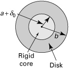
8.20. A thin circular disk of inner radius a and outer radius b is shrunk onto a rigid plug of radius a + δo (Fig. P8.20). Determine (a) the interface pressure; (b) the radial and tangential stresses.
8.21. When a steel sleeve of external diameter 3b is shrunk onto a solid steel shaft of diameter 2b, the internal diameter of the sleeve is increased by an amount δ0. What reduction occurs in the diameter of the shaft? Let ![]() .
.
8.22. A cylinder of inner diameter b is shrunk onto a solid shaft. Find (a) the initial difference in diameters if the contact pressure is p and the maximum tangential stress is 2p in the cylinder and (b) the axial compressive load that should be applied to the shaft to increase the contact pressure from p to p1. Let ![]() .
.
8.23. A brass solid cylinder is a firm fit within a steel tube of inner diameter 2b and outer diameter 4b at a temperature T1°C. If now the temperature of both elements is increased to T2°C, find the maximum tangential stresses in the cylinder and in the tube. Take αs = 11.7 × 10⁻⁶/°C, αb = 19.5 × 10⁻⁶/°C, and ![]() , and neglect longitudinal friction forces at the interface.
, and neglect longitudinal friction forces at the interface.
8.24. A thick-walled, closed-ended cylinder of inner radius a and outer radius b is subjected to an internal pressure pi only (Fig. P8.24). The cylinder is made of a material with permissible tensile strength σall and shear strength τall. Determine the allowable value of pi. Given: a = 0.8 m, b = 1.2 m, σall = 80 MPa, and τall = 50 MPa.
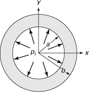
8.25. A thick-walled cylindrical tank of inner radius a and outer radius b is made of ASTM A-48 cast iron (see Table D.1) having a modulus of elasticity E and Poisson’s ratio of v. Calculate the maximum radial displacement of the tank, if it is under an internal pressure of pi, as illustrated in Fig. P8.24. Given: a = 0.5 m, b = 0.8 m, pi = 60 MPa, E = 70 GPa and v = 0.3.
8.26. A steel cylinder (σyp = 350 MPa) having inner radius a and outer radius 3a is subjected to an internal pressure pi (Fig. P8.24). Find the limiting values of the pi, using (a) the maximum shear stress theory; (b) the maximum energy of distortion theory.
8.27. A cylinder with inner radius a and outer radius 2a is subjected to an internal pressure pi (Fig. P8.24). Determine the allowable value of pi, applying (a) the maximum principal stress theory; (b) the Coulomb–Mohr theory. Assumptions: The cylinder is made of aluminum of σu = 320 MPa and ![]() .
.
8.28. A bronze bushing 60 mm in outer diameter and 40 mm in inner diameter is to be pressed into a hollow steel cylinder of 120-mm outer diameter. Calculate the tangential stresses for steel and bronze at the boundary between the two parts. Given: Eb = 105 GPa, Es = 210 GPa, v = 0.3. Assumption: The radial interference is equal to δ = 0.05 mm.
8.29. A cast-iron disk is to be shrunk on a 100-mm-diameter steel shaft. Find (a) the contact pressure; (b) the minimum allowable outside diameter of the disk. Assumption: The tangential stress in the disk is limited to 80 MPa. Given: The radial interference is δ = 0.06 mm, Ec = 100 GPa, Es = 200 GPa, and v = 0.3.
8.30. A cast-iron cylinder of outer radius 140 mm is to be shrink-fitted over a 50-mm-radius steel shaft. Find the maximum tangential and radial stresses in both parts. Given: Ec = 120 GPa, vc = 0.2, Es = 210 G Pa, vs = 0.3. Assumption: The radial interference is δ = 0.04 mm.
8.31. In the case of which a steel disk (v = 0.3) of external diameter 4b is shrunk onto a steel shaft of diameter of b, internal diameter of the disk is increased by an amount λ. Find the reduction in the diameter of the shaft.
8.32. A gear of inner and outer radii 0.1 and 0.15 m, respectively, is shrunk onto a hollow shaft of inner radius 0.05 m. The maximum tangential stress induced in the gear wheel is 0.21 MPa. The length of the gear wheel parallel to shaft axis is 0.1 m. Assuming a coefficient of static friction of f = 0.2 at the common surface, what maximum torque may be transmitted by the gear without slip?
Sections 8.6 through 8.13
8.33. A solid steel shaft of radius b is pressed into a steel disk of outer radius 2b and the length of hub engagement t = 3b (Figure 8.11). Calculate the value of the radial interference in terms of b. Given: The shearing stress in the shaft caused by the torque that the joint is to carry equals 120 MPa; E = 200 GPa, and f = 0.2.
8.34. A cast-iron gear with 100-mm effective diameter and t = 40 mm hub engagement length is to transmit a maximum torque of 120 N · m at low speeds (Fig. 8.11). Determine (a) the required radial interference on a 20-mm diameter steel shaft; (b) the maximum stress in the gear due to a press fit. Given: Ec = 100 GPa, Es = 200 GPa, v = 0.3, and f = 0.16.
8.35. Show that for an annular rotating disk, the ratio of the maximum tangential stress to the maximum radial stress is given by
(P8.35)
8.36. Determine the allowable speed ωall in rpm of a flat solid disk employing the maximum energy of distortion criterion. The disk is constructed of an aluminum alloy with σyp = 260 MPa, ![]() , ρ = 2.7 kN · s2/m4, and b = 125 mm.
, ρ = 2.7 kN · s2/m4, and b = 125 mm.
8.37. A rotating flat disk has 60-mm inner diameter and 200-mm outer diameter. If the maximum shearing stress is not to exceed 90 MPa, calculate the allowable speed in rpm. Let ν = 1/3 and ρ = 7.8 kN · s2/m4.
8.38. A flat disk of outer radius b = 125 mm and inner radius a = 25 mm is shrink-fitted onto a shaft of radius 25.05 mm. Both members are made of steel with E = 200 GPa, ν = 0.3, and ρ = 7.8 kN · s2/m4. Determine (a) the speed in rpm at which the interface pressure becomes zero and (b) the maximum stress at this speed.
8.39. A flat annular steel disk (ρ = 7.8 kN · s2/m4, ν = 0.3) of 4c outer diameter and c inner diameter rotates at 5000 rpm. If the maximum radial stress in the disk is not to exceed 50 MPa, determine (a) the radial wall thickness and (b) the corresponding maximum tangential stress.
8.40. A flat annular steel disk of 0.8-m outer diameter and 0.15-m inner diameter is to be shrunk around a solid steel shaft. The shrinking allowance is 1 part per 1000. For ν = 0.3, E = 210 GPa, and ρ = 7.8 kN · s2/m4, determine, neglecting shaft expansion, (a) the maximum stress in the system at standstill and (b) the rpm at which the shrink fit will loosen as a result of rotation.
8.41. Show that in a solid disk of diameter 2b, rotating with a tangential velocity v, the maximum stress is ![]() . Take
. Take ![]() .
.
8.42. A steel disk of 500-mm outer diameter and 50-mm inner diameter is shrunk onto a solid shaft of 50.04-mm diameter. Calculate the speed (in rpm) at which the disk will become loose on the shaft. Take ν = 0.3, E = 210 GPa, and ρ = 7.8 kN · s2/m4.
8.43. Consider a steel rotating disk of hyperbolic cross section (Fig. 8.13) with a = 0.125 m, b = 0.625 m, ti = 0.125 m, and to = 0.0625 m. Determine the maximum tangential force that can occur at the outer surface in newtons per meter of circumference if the maximum stress at the bore is not to exceed 140 MPa. Assume that outer and inner edges are free of pressure.
8.44. A steel turbine disk with b = 0.5 m, a = 0.0625 m, and to = 0.05 m rotates at 5000 rpm carrying blades weighing a total of 540 N. The center of gravity of each blade lies on a circle of 0.575-m radius. Assuming zero pressure at the bore, determine (a) the maximum stress for a disk of constant thickness and (b) the maximum stress for a disk of hyperbolic cross section. The thickness at the hub and tip are ti = 0.4 m and to = 0.05 m, respectively. (c) For a thickness at the axis ti = 0.02425 m, determine the thickness at the outer edge, to, for a disk under uniform stress, 84 MPa. Take ρ = 7.8 kN · s2/m4 and g = 9.81 m/s2.
8.45. A solid, thin flat disk is restrained against displacement at its outer edge and heated uniformly to temperature T. Determine the radial and tangential stresses in the disk.
8.46. Show that for a hollow disk or cylinder, when subjected to a temperature distribution given by T = (Ta – Tb) ln (b/r)/ln (b/a), the maximum radial stress occurs at
(P8.46)
8.47. Calculate the maximum thermal stress in a gray cast-iron cylinder for which the inner temperature is Ta = –8°C and the outer temperature is zero. Let a = 10 mm, b = 15 mm, E = 90 GPa, α = 10.4 × 10⁻⁶ per °C, and ν = 0.3.
8.48. Verify that the distribution of stress in a solid disk in which the temperature varies linearly with the radial dimension, T(r) = T0(b – r)/b, is given by
(P8.48)
Here T0 represents the temperature rise at r = 0.
8.49. Redo Example 7.12 with the element shown in Fig. 7.26 representing a segment adjacent to the boundary of a sphere subjected to external pressure p = 14 MPa.
8.50. A cylinder of hydraulic device having inner radius a and outer radius 4a is subjected to an internal pressure pi. Using a finite element program with CST (or LST) elements, determine the distribution of the tangential and radial stresses. Compare the results with the exact solution shown in Fig. 8.4a.
8.51. A cylinder of a hydraulic device with inner radius a and outer radius 4a is under an external pressure po. Employing a finite element computer program with CST (or LST) elements, calculate the distribution of tangential and radial stresses.
8.52. Redo Prob. 8.51 if the cylinder is under an internal pressure pi. Compare the results with the exact solution shown in Fig. 8.4.
8.53. Resolve Prob. 8.51 for the case in which the cylinder is subjected to internal pressure pi and external pressure po = 0.5pi.