Chapters 8–11 developed several different regression models for time series variables. Throughout, we were always interested in the variables themselves. For instance, we were interested in explaining stock or bond returns, exchange rates and yield spreads. However, there are many cases where we are not interested in the variables themselves, but in their volatility (measured by the variance). For instance, in Chapter 4 we introduced the capital asset pricing model (CAPM) and discussed how risk was important for investment decisions. The risk of investing in the stock of a company was related to the volatility of its share price (and other factors).
Another very important field of research relates to the pricing of financial derivatives (e.g. options and other securities whose payoff is derived from the price of an underlying asset). If you have studied the theory of finance, you may be aware of the Black–Scholes option price formula and other similar derivative pricing methods. In this book, we will not derive such formulae. We note only that, in these formulae, the volatility of the price of the underlying asset plays a crucial role. The methods introduced in this chapter are commonly used to provide estimates of this volatility.
We begin our discussion of volatility in asset prices informally, staying with familiar regression methods. We then discuss a very popular method for estimating financial volatility called autoregressive conditional heteroskedasticity (ARCH). The ARCH model shares a great deal of intuition with the regression model (including the AR model), but is not exactly the same as a regression model. Accordingly, methods like OLS cannot be used with ARCH. However, many computer software packages (e.g. Stata, E-views, MicroFit, etc.) can estimate ARCH models. So the fact that the theory underlying the estimation of ARCH models is difficult need not preclude your using them in practice. This chapter also discusses some extensions of ARCH models.
To provide some intuition, recall our discussion of the random walk model in Chapter 9. We defined the model as:
or
We then noted that there were good reasons for believing that such a model might be appropriate for measuring economic phenomena like stock prices or exchange rate. In other words, the stock return (exclusive of dividends) was unpredictable.
The simple random walk model is a little unreasonable as a description of stock price behavior since stocks do appreciate in value over time. A slightly more realistic model is:
This model can be interpreted as implying that stock prices, on average, increase by a per period, but are otherwise unpredictable. Known as the random walk with drift model, it adds an intercept to the random walk model, thus allowing stock prices to "drift" upwards over time (if α > 0). Equivalently, stock returns are on average α but are otherwise unpredictable.
In the rest of this section, we will assume that the random walk model for an asset price is the correct one. That is, we will assume that either the asset price follows a pure random walk or that it follows a random walk with drift, and that we have taken deviations from the mean. To avoid confusion, we will let Δyt indicate the series with deviations from means taken (i.e. Δyt = ΔYt − Δ
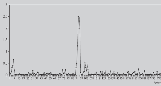
Although the ARCH model provides a better definition for volatility, it is possible to simply use Δy2t as an estimate of volatility at time t. To motivate this choice, note that high volatility is associated with big changes, either in a positive or in a negative direction. Since any number squared becomes positive, large rises or large falls in the price of an asset will imply Δy2t, is positive and large. In contrast, in stable times the asset price will not be changing much and Δy2t will be small. Hence, our measure of volatility will be small in stable times and large in chaotic times.
An alternative motivation for our measure of volatility can be obtained by recalling some material from Chapter 2. There we stressed that variance is a measure of the volatility of a variable. In general, it is common practice to equate the two and use variance as a measure of volatility. But using the variance as a measure of volatileity presents problems in the present context. A key point here is that we want to allow the volatility of an asset to change over time. The volatility at time t might be different from that at time t – 1 or t + 1, etc. In Chapter 2, we used all observations to provide one estimate of the variance. Here we can use only the observation at time t to provide an estimate of the variance at time t. (In other words, it makes no sense to use data at time t + 1 to estimate the variance at time t since the variance might be different in the two periods.)
If you: (i) note that we can only use one observation to estimate the variance; (ii) note that we have assumed the data is in deviations from mean form and, hence, has mean zero; and (iii) use the formula for the variance from Chapter 2, then you obtain Δy2t as an estimate of the variance.[81]
You can calculate this measure of volatility of an asset price quite easily in any spreadsheet or statistical computer package simply by differencing the stock price data, taking deviations from means and then squaring it. Once this is done, you will have a new time series variable – volatility – which you can then analyze using the tools introduced earlier.
Autoregressive models are commonly used to model "clustering in volatility", which is often present in financial time series data. Consider, for instance, an AR(1) model that uses volatility as the time series variable of interest:
This model has volatility in a period depending on volatility in a previous period. If, for instance, φ > 0 then if volatility was unusually high last period (e.g. Δy2t−1 was very large), it will also tend to be unusually high this period. Alternatively, if volatility was unusually low last period (e.g. Δy2t−1 was near zero) then this period's volatility will also tend to be low. In other words, if the volatility is low it will tend to stay low, if it is high it will tend to stay high. Of course, the presence of the error, et, means that there can be exceptions to this pattern. But, in general, this model implies that we will tend to observe intervals or clusters in time where volatility is low and intervals where it is high. In empirical studies of asset prices, such a pattern is very common. As an example, recall that in Chapter 2, we plotted the £/$ exchange rate (see Figure 2.1). If you look back at this figure, you can see long spells when the exchange rate changed very little (e.g. 1949–1967 and 1993–1996) and other, longer spells (e.g. 1985–1992) where it was more volatile.
The previous discussion refers to the AR(1) model, but it can be extended to the AR(p) model. All of the intuition given in Chapter 9 is relevant here. The only difference is that the interpretation relates to the volatility of the series rather than to the series itself. Furthermore, all of the statistical techniques we described in Chapter 9 are relevant here. Provided the series is stationary (e.g. |φ| < 1 in the AR(1) case), then OLS estimates and P-values can be interpreted in the standard way. Testing for a unit root can be conducted using a Dickey–Fuller test. In short, there is nothing statistically new here.
The class of ARCH models (including extensions) is probably the most popular one for working with financial volatility. It is most compactly explained by working with the familiar regression model:
Note that this general model contains many of the other models we have been working with. For instance, if Xjt = Yt−j (i.e. the explanatory variables are lags of the dependent variable) then this is an AR model. Another interesting case we will focus on below occurs if there are no explanatory variables at all (i.e. α = β1 = ... = βk = 0) in which case the ARCH model we will describe shortly simply relates to the dependent variable itself. If we set this dependent variable to be the demeaned stock returns (i.e. Δyt = ΔYt − Δ
The ARCH model relates to the variance (or volatility) of the error, et. You may wish to review the material at the end of Chapter 2 if you have forgotten the properties of variances. To simplify notation (and adopt a very common notation in financial econometrics), we will let:
In other words, σ2t will be our notation for volatility. It is this which is crucial in many financial applications. Note that we are allowing volatility to vary over time – which is quite important in light of our previous discussion of clustering of volatility.
The ARCH model with p lags (denoted by ARCH(p)) assumes that today's volatility is an average of past errors squared:
where γ1, ..., γp are coefficients that can be estimated in many statistical software packages. In the case where we have no explanatory variables and the dependent variable is Δyt, we have
and the ARCH volatility depends on recent values of Δy2t – the metric for volatility we were using in the first half of this chapter. This model is closely related to the autoregressive model (which accounts for the "AR" part of the name ARCH) and ARCH models have similar properties to AR models – except that these properties relate to the volatility of the series.
There are many extensions of the ARCH model that are used by financial analysts. For instance, Stata lists seven different variants of the ARCH model with acronyms like GARCH, SAARCH, TARCH, AARCH, NARCH and NARCHK. Another popular alternative model, which is not in the ARCH class is called stochastic volatility. If you are doing a great deal of work on financial volatility, you should do further study to learn more about these models. Here we will only introduce the most popular of these extensions: Generalized ARCH or GARCH. This takes the ARCH model and adds on lags of the volatility measure itself (instead of just adding lags of squared errors). Thus, a GARCH model with (p, q) lags is denoted by GARCH(p, q) and has a volatility equation of:
The properties of the GARCH model are similar to the ARCH model. For instance, the coefficients can be interpreted in a similar fashion to AR coefficients and related to the degree of persistence in volatility. However, it can be shown that the GARCH model is much more flexible, much more capable of matching a wide variety of patterns of financial volatility.
Many time series variables, particularly asset prices, seem to exhibit random walk behavior. For this reason, it is hard to predict how they will change in the future. However, such variables often do exhibit predictable patterns of volatility.
The square of the change in an asset price is a measure of its volatility.
Standard time series methods can be used to model the patterns of volatility in asset prices. The only difference is that volatility of the asset price is used as the dependent variable.
ARCH models are a more formal way of measuring volatility. They contain two equations. One is a standard regression equation. The second is a volatility equation, where volatility is defined as being the (time varying) variance of the regression error.
ARCH models share similarities with AR models, except that the "AR" part relates to the volatility equation.
There are many extensions of ARCH, of which GARCH is the most popular.
ARCH and GARCH models can be estimated using many common statistical software packages (but are hard to work with using a spreadsheet).
[81] In deriving this result we have ignored the N - 1 term in the denominator in the formula introduced in Chapter 2. You should simply note that it is not important here. In some formulas for the variance, N - 1 is replaced by N. Here, N = 1 so we can just ignore it.
[82] This follows from the fact that ln(24.53) is 3.200 and ln(30.14) is 3.406.


