
In Excel, you use formulas. A formula is an equation that performs a calculation. A formula can consist of operators, functions, numbers, text, and cell references. You place formulas in cells. You can click a cell and then type your formula into the formula bar or you can type your formula directly into a cell. You start most formulas by typing an equal sign (=).
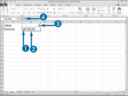
The real power of Excel comes from its ability to manipulate information and perform mathematical calculations. When calculating, you can use operators such as the plus (+), minus (–), multiplication (*), and division (/) signs. You start by typing an equal sign, followed by the values you want to add, subtract, multiply, or divide, each separated by an operator. For example, type =6*3/2-B1, and then press Enter. Excel does the math and displays the answer.
You can also include a value in a formula by clicking in the cell that contains the value. For example, if the value you want to include in your formula is in cell B1, type an equal sign (=) and then click in cell B1 type an operator and then continue creating your formula.

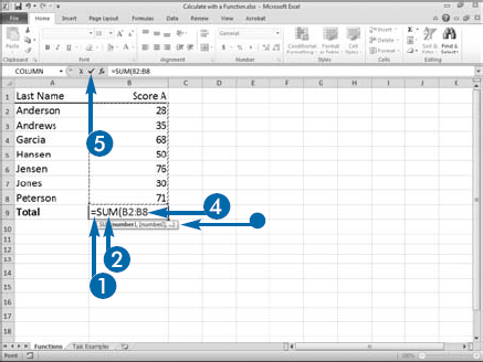
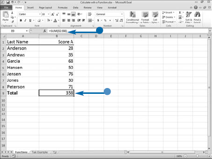
A function is a prewritten formula. You enter a value or values into a function; it performs the calculation and returns the result to you. Functions simplify and shorten long formulas. For example, instead of entering =B2+B3+ B4+B5+B6+B7, you can use the SUM function and enter =SUM(B2:B7). You can use a function alone, combine it with other functions, or embed it in a formula. All of the following formulas are valid: =2*SUM(B2:B7) multiplies the sum of cells B2 through B7 by 2; =ROUND(SUM(G2:G8),2) rounds the sum of G2 through G8 to 2 decimal places; and =SUM(B2:B8)+SUM(C2:C8) adds the sum of B2 through B8 to the sum of C2 through C8.
When a function begins a formula, it must be preceded by an equal sign. You type the equal sign followed by the function name and parentheses. As you begin to typing the formula name, the AutoComplete list appears. The AutoComplete list lists all functions. You double-click a function name to select it. You call the values that you enter into a function arguments. Place arguments inside the parentheses separated by commas. Arguments can be numbers, text, logical values, dates, arrays, error values, cells, or cell ranges.
Excel has a large number of functions from which you can choose. They are divided into categories, such as Statistical, Financial, and Date and Time. For a description of each function, click the Help button, and then click Function Reference. The functions are listed by category. The function description explains each function and describes each argument. Arguments can be constants or formulas. Some functions have arguments that are optional.
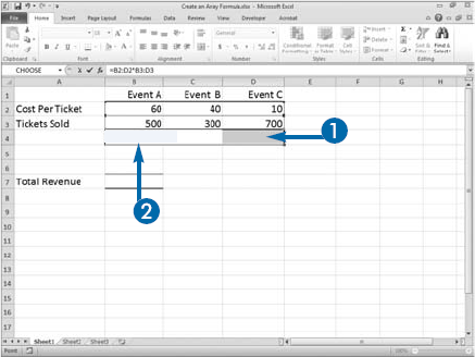
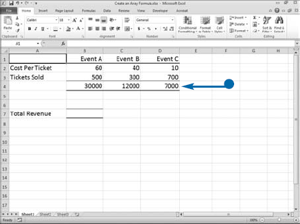
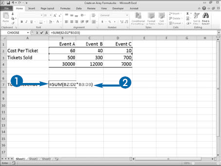
If your find yourself repeatedly entering the same formula into adjacent cells and only changing the cell reference, you should consider using an array formula. With an array formula, you can enter a formula once and have it apply to multiple cells. In addition, array formulas use less memory.
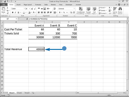
Array formulas differ from regular formulas in that they can produce multiple results from a single formula. They are easy to recognize because curly braces always surround them. When you complete an array formula, you press Ctrl+Shift+Enter and Excel places the curly braces around the formula. You cannot create and array formula by typing curly braces. You must press Ctrl+Shift+Enter. Make sure you are holding down both the Ctrl and Shift keys when you press Enter. If you are only pressing the Shift key, Excel enters a regular formula in the active cell. If you are only pressing the Ctrl key, Excel enters a regular formula in all the selected cells.
There are two types of array formulas: multi-cell formulas and single cell formulas. An array formula that places results in multiple cells is called a multi-cell formula. An array formula that places results in a single cell is called a single-cell formula. When you calculate a multi-cell formula, you place the results of the formula in multiple cells. When you calculate a single-cell formula, you place the results in a single cell.
The formula {=C2:E2*C3:E3} performs the following three calculation: C2*C3, D2*D3, and E2*E3 and places the results of each calculation in separate cell. The formula {=SUM(C2:E2*C3:E3)} performs the same three calculations, sums the results of the calculations and places that result in a single cell.
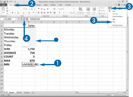
Excel's AutoSum feature offers instant access to the following functions: SUM, AVERAGE, MIN, MAX, and COUNT. The SUM function adds the numeric values in the selected range, the AVERAGE function finds the average of the numeric values in the selected range, the MIN function finds the lowest numeric value in the selected range, the MAX function finds the highest numeric value in the selected range, and the COUNT function counts the numeric values in the selected range. To use these functions, select a range and then select the AutoSum option you want. Excel places the result in the first available adjacent cell, generally to the right of a horizontal selection or below a vertical selection. Or, you can select a function and let Excel select the range. You can change Excel's selection.

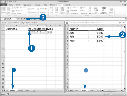
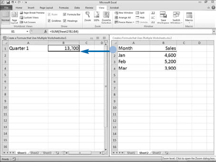
You can create formulas that reference other worksheets. For example, if you base your calculations on raw data, you can keep that data in a separate worksheet and reference it when needed. To reference cells in another worksheet, precede the cell address with the worksheet name followed by an exclamation point (!). For example, you can place the following formula in a cell in Sheet1 and use it to sum cells in Sheet2: =SUM(Sheet2!B2:B4). You can type the sheet reference, or you can select Sheet2 and then click and drag to reference cells B2 to B4. If you change the worksheet name, Excel automatically updates the formula. To learn how to change the worksheet name, see Chapter 3.
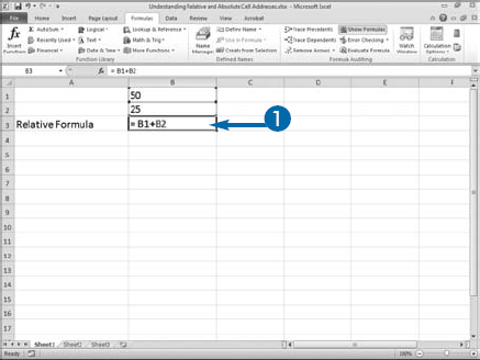
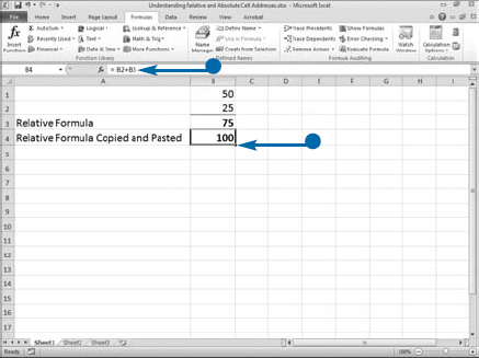
When you create a formula, you can refer to cells by using relative, absolute, or mixed cell addresses. The type of address you use is important when you copy the formula to another cell. When you use a relative cell address, the formula is based on the position of cells used in the formula relative to the cell where the formula is located. For example, if you enter the formula = B1+B2 in cell B3, Excel moves up two cells to cell B1 and gets that value and then moves up one cell to cell B2 and adds that value to the first value. If you copy the formula, Excel will always move up two cells to get the first value and up one cell to get the second value. So, if you copy the formula to cell B4, the formula automatically becomes =B2+B3. In most instances, by default, formulas use relative cell addresses.
When you use an absolute cell address, the formula is always based on the exact cell you enter into to the formula. For example, if you enter the formula =$D$1+$D$2 in cell D3, Excel adds cell D1 to cell D2. If you copy the formula, Excel will still add cell D1 to cell D2. You make a cell address absolute by placing a dollar sign in front of the column and row reference.
You can have a mixed cell address. With a mixed cell address, either the column stays the same and the row changes – an absolute column and a relative row – or the row stays the same and the column changes – an absolute row and a relative column. You can press the F4 key to cycle through absolute, relative, and mixed cell addresses.
Understanding Relative and Absolute Cell Addresses
Use a Relative Cell Address


Excel copies the formula in a relative fashion.


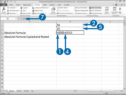
Excel copies the cell in an absolute fashion.

Extra
To use the same formula in multiple cells, you can use the Fill Handle to copy the formula to adjoining cells in the same row or column. This changes all relative cell references within the formula. For example, copying =SUM(A1:A5) from cell A6 to cell B6 results in =SUM(B1:B5). The Fill Handle is the black box on the bottom-right corner of a selected cell. You simply drag it to an adjacent range of cells. Excel copies the formula and any cell formatting to the new cells.
When you move a formula to a new cell on your worksheet, all cell references in the formula, whether absolute or relative, remain the same. For example, if you move the formula =SUM(A1:A5), which has a relative reference and is located in cell A6, into cell A7, the cell references in the formula do not change. You can move a formula simply by dragging it to a new cell. Hover your mouse pointer over the border of the cell; when you see a four-sided arrow (
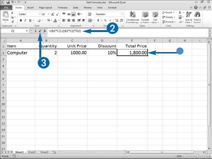
After creating a formula, you can update it to accommodate new data. You can change the cells your formula references or change the arguments in your function. For example, if the method of calculation changes, you can edit the formula. Or, if you need to make changes to a function, you can.
You can edit your formula directly, or, if your formula is a function, you can edit it using the Function Arguments dialog box. To edit a formula directly, double-click in the cell containing the formula and then type your changes or double-click in the cell containing the formula, and then use the formula bar to make your changes. When you double-click in a cell, Excel enters Edit mode — you can see the word Edit on the left side of the status bar. When Excel is in Edit mode, it highlights the cells the formula references. The highlight for each value and range displays in a different color.
You can change function arguments by clicking in the cell that contains the function and then clicking the Insert Function (fx) button to open the Function Arguments dialog box. In the Function Arguments dialog box you can change the value or select new cell ranges for each argument. When you click OK to accept the changes, Excel updates the results.
You can use the same method you use to edit formulas to edit text. Just double-click in the cell you want to edit and then type your changes or use the formula bar to make your changes.


Extra
You can use cut, copy, and paste to move a formula from one location in your worksheet to another location. When you cut and paste a formula, the cell references do not change. This is true for formulas with relative cell addresses and for formulas with absolute cell addresses. When you copy and paste a formula, the cell references may change depending upon the type of cell reference. See Chapter 3 to learn how to cut, copy, and paste.
To delete a formula, click in the cell that contains the formula and then press the Delete key. Or click the Home tab. Click the
You can edit a formula by clicking in the cell that contains the formula, pressing F2, and then making your changes. Pressing F2 while you are in a cell, places you in Edit mode.
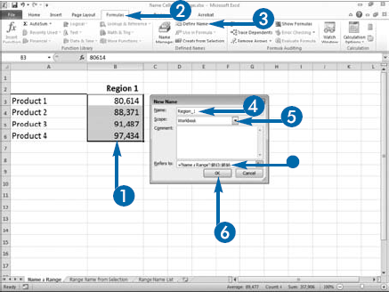
In Excel, you can name individual cells, or groups of cells called ranges. A cell named Tax_Rate or a range named Region_1 is easier to remember than the corresponding cell address or range. You can use named cells and ranges in formulas to refer to the values contained in them. When you move a named range to a new location, Excel automatically updates any formulas that refer to it.
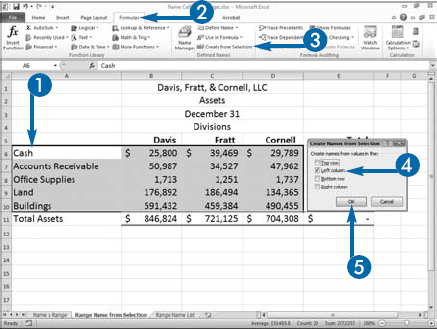
When you name a range, you determine the scope of the name by telling Excel whether it applies to a particular worksheet or the entire workbook. You can name several ranges at once by using Excel's Create from Selection option.
Excel range names must be fewer than 255 characters. The first character must be a letter, underscore (_), or backslash (). You cannot use spaces or symbols. You can use the period or underscore as a separator. It is best to create short, memorable names. Each range name must be unique within it scope. Range names are not case sensitive. Excel considers the name cash the same as the name CASH.
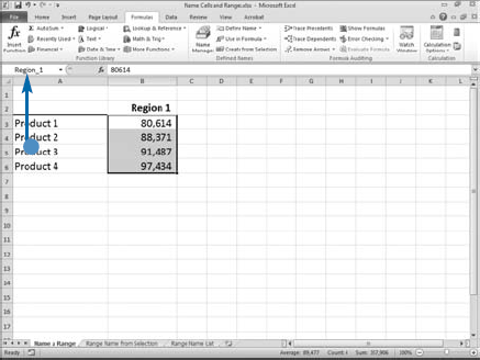
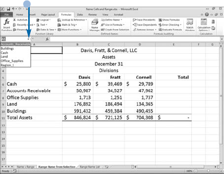
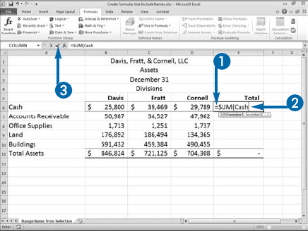
There is a down arrow located on the left side of the formula bar. When you click the down arrow, a list of named ranges appears. If you click a named range, you will move to the cells it defines. When you are creating a formula, if you click and drag to select a group of cells that have a range name, Excel automatically uses the range name instead of the cell address.
To learn how to use a named range, see the section "Create Formulas That Include Names" later in this chapter.
Use a constant whenever you want to apply the same value in different contexts. With constants, you can refer to a value by simply using the constant's name.
You can use constants in many ways. For example, the sales tax rate is a familiar constant that, when multiplied by the subtotal on an invoice, results in the tax owed. Likewise, income tax rates are the constants used to calculate tax liabilities. Although tax rates change from time to time, they tend to remain constant within a tax period.
To create a constant in Excel, you need to type its value in the New Name dialog box, the same dialog box you use to name ranges, as shown in the previous section, "Name Cells and Ranges." When you define a constant, you determine the scope of the constant by telling Excel whether it applies to the current worksheet or the entire workbook. To use the constant, simply use the name you defined.
The rules that apply to naming a range also apply to naming a constant. Excel constant names must be fewer than 255 characters. The first character must be a letter, underscore (_), or backslash (). You cannot use spaces or symbols. You can use the period or underscore as a separator. It is best to create short, memorable names. Each name must be unique within its scope. Constant names are not case sensitive. Excel considers the name tax the same as the name TAX.
To learn how to use a constant, see the next section, "Create Formulas That Include Names."
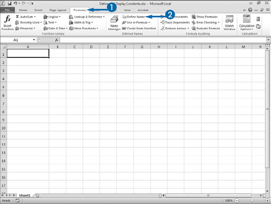
Define and Display Constants
Define a Constant
The New Name dialog box appears.
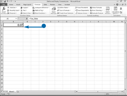
You can now use the constant.

The Autocomplete list appears.
Note: If you do not know the constant's name, click the Formulas tab and then click Use in Formula. A menu appears. Click the name.

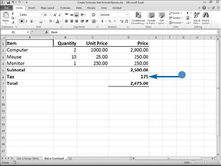
The constant's value appears in the cell.
Note: To learn how to use named constants and named ranges in formulas, see the next section, "Create Formulas That Include Names."
Constructing formulas can be complicated, especially when you use several functions in the same formula or when multiple arguments are required in a single function. Using named constants and named ranges can make creating formulas and using functions easier by enabling you to use terms you have created that clearly identify a value or range of values.
An argument is information you provide to the function so the function can do its work. A named constant is a name you create that refers to a single, frequently used value. See the previous section, "Define and Display Constants," for more information. A named range is a name you assign to a group of related cells. See the section "Name Cells and Ranges," earlier in this chapter, for more information. To insert a name into a function or use it in a formula or as a function's argument, you must type it, access it by clicking Use in Formula on the Formulas tab, or select it from the Function AutoComplete list.
When you name a range, the name must be unique within its scope. When you define the same range name globally and/or for multiple worksheets, by default Excel uses the definition you created for the active worksheet. If you want to use the global definition, you must precede the name with the workbook name followed by an exclamation point (!); for example, WorkBookName!RangeName. If you want to use a definition created for another worksheet, you must precede the name with the worksheet name followed by an exclamation point (!); for example, WorkSheetName!ConstantName.
Create Formulas that Include Names
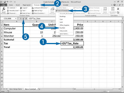
Use a Constant or Range Name in a Formula
As you type, a list of possible values appears. Double-click a value to place it in the formula.
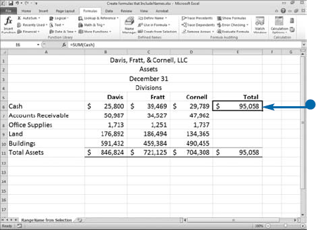
Excel calculates the result.
Use a Constant or Range Name in a Formula
Note: Use this technique if you forget the name of a constant or range.
A menu appears.
If necessary, continue typing your formula.
Excel calculates the results.
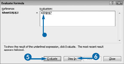
When you create formulas, you can nest one formula within another formula. Because there are so many intermediate steps when you nest formulas, determining the accuracy of your results may be difficult. You can use the Evaluate Formula dialog box to check the result of intermediate calculations to determine if your result is correct.
When you open the Evaluate Formula dialog box, you see your formula. The Evaluate Formula dialog box steps you through the calculation one expression at a time so you can see how Excel evaluates each expression. Click the Evaluate button to begin the process. When your formula includes a function, Excels solves for each argument in the function, and then solves the rest of the formula. Excel underlines individual expressions. You can click the Evaluate button to see the results of an expression. The results of expressions appear in italics.
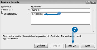
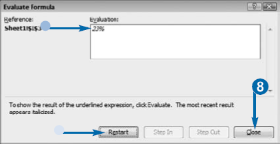
If you based the reference on another formula, you can click the Step In button to display the formula. Click the Step Out button to return to the reference. When you have stepped through the entire formula, Excel displays the result and a Restart button. Click the Restart button to evaluate your expression again.
You cannot modify your formula while you are in the Evaluate Formula dialog box. If you find an error and you want to change to your formula, close the Evaluate Formula dialog box to make the change.
If you want to examine all the formulas in your worksheet, click the Show Formulas button in the Formula Auditing group of the Formulas tab. To return to displaying results, click the Show Formulas button again.


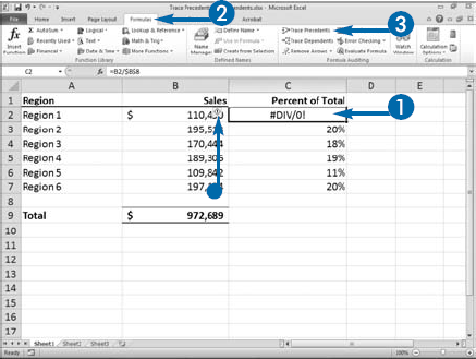
When you create a formula, Excel evaluates all the values in the formula and returns a result. If Excel cannot calculate the formula, it displays an error message in the formula cell. You can use the Excel trace features to help you locate your error.
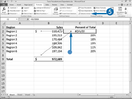
Typically, an error occurs when your formula refers to an invalid cell value. For example, if the cell contains the formula =B2/$B$8 and cell B8 contains the number 0 or is blank, Excel returns the error message #DIV/0!, which indicates that the formula attempted to divide by zero.
You can view a graphical representation of the cells a formula refers to by clicking in the cell and then clicking Trace Precedents in the Formula Auditing group on the Formulas tab. This option draws blue arrows to each cell referenced in the formula, so you can identify the exact cells used in the formula.
If you want to find out which formulas use a specific cell, you can view a graphical representation by clicking in the cell and then clicking Trace Dependents in the Formula Auditing group on the Formulas tab. This option draws blue arrows to each cell that contains a formula that uses the active cell as an argument. By displaying the dependent cells for a formula, you can visually identify the cells that require the formula. If you perform this option before deleting a value, you can quickly determine if your deletion will affect any formulas on your worksheet.
You can remove arrows Excel draws to dependents or precedents by clicking Remove Arrows in the Formula Auditing group on the Formulas tab.
Trace Precedents and Dependents
Trace Precedents
If the cell has an error, an Error icon displays next to the formula.
Excel draws arrows between the cells on which the formula is based and the formula's cell.
Excel removes the arrows.
Note: Click the

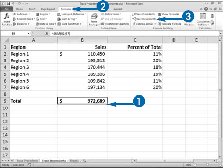
Excel draws arrows between the formula's cell and the dependent cells.
Excel removes the arrows.
Note: Click the

