10
Scoring rules

In Chapter 2 we studied coherence and explored relations between “acting rationally” and using probability to measure uncertainty about unknown events. De Finetti’s “Dutch Book” theorem guaranteed that, if one wants to avoid a sure loss (that is, be coherent), then probability calculus ought to be used to represent uncertainty. The conclusion was that, regardless of one’s beliefs, it is incoherent not to express such beliefs in the form of some probability distribution. In our discussion, the relationship between the agent’s own knowledge and expertise, empirical evidence, and the probability distribution used to set fair betting odds was left unexplored. In this chapter we will focus on two related questions. The first is how to guarantee that probability assessors reveal their knowledge and expertise about unknowns in their announced probabilities. The second is how to evaluate, after events have occurred, whether their announced probabilities are “good.”

To make our discussion concrete, we will focus on a simple situation, in which assessors have a clear interest in the quality of their announced probabilities. The prototypical example is forecasting. We will talk about weather forecasting, partly because it is intuitive, and partly because meteorologists were among the first to realize the importance of this problem. Weather forecasting is a good example to illustrate these concepts, but clearly not the only application of these ideas. In fact, any time you are trying to empirically compare different prediction algorithms or scientific theories you are in a situation similar to this.

In a landmark paper, Brier described the issue as follows:

We will study these questions formally by considering the measures used for the evaluation of forecasters. We will talk about scoring rules. In relation to our discussion this far, these can be thought of as loss functions for the decision problem of choosing a probability distribution. The process by which past data are used in reaching a prediction is not formally modeled—in contrast to previous chapters whose foci were decision functions. However, data will come into play in the evaluation of the forecasts.

Featured articles:

Brier, G. (1950). Verification of forecasts expressed in terms of probability, Monthly Weather Review 78: 1–3.

Good, I. J. (1952). Rational decisions, Journal of the Royal Statistical Society, Series B, Methodological 14: 107–114.

In the statistical literature, the earliest example we know of a scoring rule is Good (1952). Winkler (1969) discusses differences between using scoring rules for assessing probability forecasts and using them for elicitation. A general discussion of the role of scoring rules in elicitation can be found in Savage (1971) and Lind-ley (1982b). Additional references and discussion are in Bernardo and Smith (1994, Sec. 2.7).

10.1 Betting and forecasting

We begin with two simple illustrations in which announcing one’s own personal probabilities will be the best thing to do for the forecaster.

The first example brings us back to the setting of Chapter 2. Suppose you are a bookmaker posting odds q : (1 – q) on the occurrence of an event θ. Say your personal beliefs about θ are represented by π. Both π and q are points in [0, 1]. As the bookmaker, you get –(1 – q)S if θ occurs, and qS if θ does not occur, where, as before, S is the stake and it can be positive or negative. Your expected gain, which in this case could also be positive or negative, is

−(1 – q)Sπ + qS(1 – π) = S(q – π).

Suppose you have to play by de Finetti’s rules and post odds at which you are indifferent between taking bets with positive or negative stakes on θ. In order for you to be indifferent you need to set q = π. So in the betting game studied by de Finetti, a bookmaker interested in optimizing expected utility will choose betting odds that correspond to his or her personal probability. On the other hand, someone betting with you and holding beliefs π′ about θ will have an expected gain of S(π′ – q) and will have an incentive to bet a positive stake on θ whenever π′ > q.

The second example is a cartoon version of the problem of ranking forecasters. Commencement day is two days away and a departmental ceremony will be held outdoors. As one of the organizers you decide to seek the opinion of an expert about the possibility of rain. You can choose among two experts and you want to do so based on how well they predict whether it will rain tomorrow. Then you will decide on one of the experts and ignore the other, at least as far as the commencement day prediction goes. You are going to come up with a rule to rank them and you are going to tell them ahead of time which rule you will use. You are worried that if you do not specify the rule well enough, they may report to you something that is not their own best prediction, in an attempt to game the system—the same concern that was mentioned by Brier earlier.

So this is what you come up with. Let the event “rain tomorrow” be represented here by θ, and suppose that q is a forecaster’s probability of rain for tomorrow. If θ occurs, you would like q to be close to 1; if θ does not occur you would like q to be close to 0. So you decide to assign to each forecaster the score (q – θ)², and then choose the forecaster with the lowest score.

With this scoring rule, is it in a forecaster’s best interest to announce his or her own personal beliefs about θ in playing this game? Let us call a forecaster’s own probability of rain tomorrow π, and compute the expected score, which is

(q – 1)²π + q²(1 – π) = (q – π)² + π(1 – π).

To make this as small as possible a forecaster must choose q = π.

Incidentally, choosing one forecaster only and ignoring the other may not necessarily be the best approach from your point of view: there may be ways of combining the two to improve on both forecasts. A discussion of that would be too long a detour, but you can look at Genest and Zidek (1986) for a review.

10.2 Scoring rules

10.2.1 Definition

We are now ready to make these considerations more formal. Think of a situation where a forecaster needs to announce the probability of a certain event. To keep things from getting too technically complex we will assume that this event has a finite number J of possible mutually exclusive outcomes, represented by the vector θ = (θ₁, ..., θ_J) of outcome indicators. When we say that θ_j occurred we mean that θ_j = 1 and therefore θ_i = 0 for i ≠ j. The forecaster needs to announce probabilities for each of the J possibilities. The vector q = (q₁, ..., q_J) contains the announced probabilities for the corresponding indicator. Typically the action space for the choice of q will be the set Q of all probability distributions in the J –1 dimensional simplex. A scoring rule is a measure of the quality of the forecast q against the observed event outcome θ. Specifically:

Definition 10.1 (Scoring rule) A scoring rule s for the probability distribution q is a function assigning a real number s(θ, q) to each combination (θ, q).

We will often use the shorthand notation s(θ_j, q) to indicate s(θ, q) evaluated at θ_j = 1 and θ_i = 0 for i ≠ j. This does not mean that the scoring rule only depends on one of the events in the partition. Note that after θ_j is observed, the score is computed based potentially on the entire vector of forecasts, not just the probability of θ_j. In the terminology of earlier lectures, s(θ_j, q) represents the loss when choosing q as the announced probability distribution, and θ_j turns out to be the true state of the world. We will say that a scoring rule is smooth if it is continuously differentiable in each q_j. This requires that small variations in the announced probabilities would produce only small variations in the score, which is often reasonable.

Because θ is unknown when the forecast is made, so is the score. We assume that the forecaster is a utility maximizer, and will choose q to minimize the expected score. This will be done based on his or her coherent personal probabilities, denoted by π = (π₁, ..., π_J). The expected loss from the point of view of the forecaster is

Note the different role played by the announced probabilities q that enter the score function, and the forecaster’s beliefs that are weights in the computation of the expected score.

The fact that the forecaster seeks a Bayesian solution to this problem does not necessarily mean that the distribution q is based on Bayesian inference, only that the forecaster acts as a Bayesian in deciding which q will be best to report.

10.2.2 Proper scoring rules

In both of our examples in Section 10.1, the scoring rule was such that the decision maker’s expected score was minimized by π, the personal beliefs. Whenever this happens, no matter what the beliefs are, the scoring rule is called proper. More formally:

Definition 10.2 (Proper scoring rule) A scoring rule s is proper if, and only if, for each strictly positive π,

If π is the only solution that minimizes the expected score, then the scoring rule is called strictly proper.

Winkler observes that this property is useful for both probability assessment and probability evaluation:

Proper scoring rules can also be used as devices for eliciting one’s subjective probability. Elicitation of expectations is studied by Savage (1971) who mathematically developed general forms for the scoring rules that are appropriate for eliciting one’s expectation.

Other proper scoring rules are the logarithmic (Good 1952)

s(θ_j, q) = −log q_j

and the spherical rule (Savage 1971)

10.2.3 The quadratic scoring rules

Perhaps the best known proper scoring rule is the quadratic rule, already encountered in Section 10.1. The quadratic rule was introduced by Brier (1950) to provide a “verification score” for weather forecasts. A mathematical derivation of the quadratic scoring rule can be found in Savage (1971). A quadratic scoring rule is a function of the form

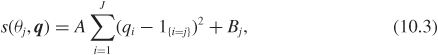
with A > 0. Here 1_{i=j} is 1 if i = j and 0 otherwise.

Take a minute to convince yourself that the rule of the commencement party example of Section 10.1 is a special case of this, occurring when J = {1, 2}. Find the values of A and B_j implied by that example, and sort out why in the example there is only one term to s while here there are J.

Now we are going to show that the quadratic scoring rule is proper; that is, that q = π is the Bayes decision. To do so, we have to minimize, with respect to q, the expected score

subject to the constraint that the elements in q sum to one. The Lagrangian for this constrained minimization is

Taking partial derivatives with respect to q_k we have

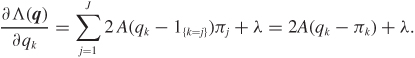
Setting q_k = π_k and λ = 0 satisfies the first-order conditions and the constraint, since ∑_j π_j = 1. We should also verify that this gives a minimum. This is not difficult, but not insightful either, and we will not go over it here.

10.2.4 Scoring rules that are not proper

It is not difficult to construct scoring rules that look reasonable but are not proper. For example, go back to the commencement example, and say you state the score |q – θ|. From the forecaster’s point of view, the expected score is

(1 – q)π + q(1 – π) = π + (1 – 2π)q.

This is linear in q and is minimized by announcing q = 1 if π > 0.5 and q = 0 if π < 0.5. If π is exactly 0.5 then the expected score is flat and any q will do. You get very little information out of the forecaster with this scoring system. Problem 10.1 gives you a chance to work out the details in the more general cases.

Another temptation you should probably resist if you want to extract honest beliefs is that of including in the score the consequences of the forecaster’s error on your own decision making. Say a company asks a geologist to forecast whether a large amount of oil is available (θ₁) or not (θ₂) in the region. Say q is the announced probability. After drilling, the geologist’s forecast is evaluated by the company according to the following (modified quadratic) scoring rule:

that is, the penalty for an error when the event is false is 10 times the penalty when the event is true. It may very well be that the losses to the company are different in the two cases, but that should affect the use the company makes of the probability obtained by the geologist, not the way the geologist’s accuracy is rewarded. To see that note that the geologist will choose q that minimizes the expected score. Because q₂ = 1 – q₁

The minimum is attained when q₁ = π/(10 – 9π). Clearly, this rule is not proper. The announced probability is always smaller than the geologist’s own probability π when π ∊ (0, 1).

One may observe at this point that as long as the announced q₁ is an invertible function of π the company is no worse off with the scoring rule above than it would be with a proper rule, as long as the forecasts are not taken at face value. This is somewhat general. Lindley (1982b) considers the case where the forecaster is scored based on the function s(θ₁, q) if θ₁ occurs, and s(θ₂, q) if θ₂ occurs. So the forecaster should minimize his or her expected score

Sq) + (1 – π)s(θ₂, q).

If the utility function has a first derivative, the forecaster should obtain q as a solution of the equation dS/dq₁ = 0 under the constraint q₂ = 1–q₁. This implies πs′(θ₁, q)+(1 – π)s′(θ₂, q) = 0. Solving, we obtain

which means that the probability π can be recovered via a transformation of the stated value q. Can any value q lead to a probability? Lindley studied this problem and verified that if q solves the first-order equation above, then its transformation obeys the laws of probability. So while a proper scoring rule guarantees that the announced probabilities are the forecaster’s own, other scoring rules may achieve the goal of extracting sufficient information to reconstruct the forecaster’s probabilities.

10.3 Local scoring rules

A further restriction that one may impose on a scoring rule is the following. When event θ_j occurs, the forecaster is scored only on the basis of what was announced about θ_j, and not on the basis of what was announced for the events that did not occur. Such a scoring rule is called local. Formally we have the following.

Definition 10.3 (Local scoring rule) A scoring rule s is local if there exist functions s_j(.), j ∊ J, such that s(θ_j, q) = s_j(q_j).

For example, the logarithmic scoring rule s(θ_j, q) = −log q_j is local. The lower the probability assigned to the observed event, the higher the score. The rest of the announced probabilities are not taken into consideration. The quadratic scoring rule is not local. Say J = 3, A = 1, and B_j = 0. Suppose we observe θ₁ = 1. The vectors q = (0.5, 0.25, 0.25) and q′ = (0.5, 0.5, 0) both assigned a probability of 0.5 to the event θ₁, but q′ gets a score of 0.5 while q gets a score of 0.375. This is because the quadratic rule penalizes a single error of size 0.5 more than it penalizes two errors of size 0.25. It can be debated whether this is appropriate or not. If you are tempted to replace the square in the quadratic rule with an absolute value, remember that it is not proper (see Problem 10.1). Another factor to consider in thinking about whether a local scoring rule is appropriate for a specific problem has to do with whether there is a natural ordering or a notion of closeness for the elements of the partition. A local rule gives no “partial credit” for near misses. If one is predicting the eye color of a newborn, who turns out to have green eyes, one may assess the prediction based only on the probability of green, and not worry about how the complement was distributed among, say, brown and blue. Things start getting trickier if we consider three events like “fair weather,” “rain,” and “snow” on a winter’s day. Another example where a local rule may not be attractive is when the events in the partitions are the outcomes of a quantitative random variable, such as a count. Then the issue of near misses may be critical.

Naturally, having a local scoring rule gives us many fewer things to worry about and makes proving theorems easier. For example, the local property leads to a nice functional characterization of the scoring rule. Specifically, every smooth, proper, and local scoring rule can be written as B_j + A log q_j for A < 0. This means that if we are interested in choosing a scoring rule for assessing probability forecasters, and we find that smooth, proper, and local are reasonable requirements, we can restrict our choice to logarithmic scoring rules. This is usually considered a very strong point in favor of logarithmic scoring rules. We will come back to it later when discussing how to measure the information provided by an experiment.

Theorem 10.1 (Proper local scoring rules) If s is a smooth, proper, and local scoring rule for probability distributions q defined over Θ, then it must be of the form s(θ_j, q) = B_j + A log q_j, where A < 0 and the B_j are arbitrary constants.

Proof: Assume that π_j > 0 for all j. Using the fact that s is local we can write

Because s is smooth, S, which is a continuous function of s, will also be smooth. Therefore, in order for π to be a minimum, it has to satisfy the first-order conditions for the Lagrangian:

Differentiating,

Because s is proper, the minimum expected score is achieved when q = π. So, if π is a minimum, it must be that

Integrating both sides of (10.7), we get that each s_j must be of the form s_j(π_j) = −λ log π_j + B_j. In order to guarantee that the extremal found is a minimum we must have λ > 0.

The logarithmic scoring rule goes back to Good, who pointed out:

We changed Good’s notation to match ours. It is interesting to see how Good specifies the constants B_j to set up a reward structure that could correspond to both a win and a loss, and what is his justification for this. It is also remarkable how Good uses the word “objective” for “true to one’s own knowledge and beliefs.” The reason for this is in what follows:

Imposing the condition that a scoring rule is local is not the only way to narrow the set of candidate proper scoring rules one may consider. Savage (1971) shows that the quadratic loss is the only proper scoring rule that satisfies the following conditions: first, the expected score S must be symmetric in π and q, so that reversing the role of beliefs and announced probabilities does not change the expected score. Second, S must depend on π and q only through their difference. The second condition highlights one of the rigidities of squared error loss: the pairs (0.5, 0.6) and (10⁻¹²,0.1 + 10⁻¹²) are considered equally, though in practice the two discrepancies may have very different implications.

We have not considered the effect of a scoring rule on how one collects and uses evidence, but it is an important topic, and we will return to this in Chapter 13, when exploring specific ways of measuring the information in a data set.

10.4 Calibration and refinement

10.4.1 The well-calibrated forecaster

In this section we discuss calibration and refinement, and their relation to scoring rules. Our discussion follows DeGroot and Fienberg (1982) and Seidenfeld (1985).

A set of probabilistic forecasts π is well calibrated if π% of all predictions reported at probability π are true. In other words, calibration looks at the agreement between relative frequency for the occurrence of an event (rain in the above context) and forecasts. Here we are using π for forecasts, and assume that π = q. To illustrate calibration, consider Table 10.1, adapted from Brier (1950). A forecaster is calibrated if the two columns in the table are close.

Requiring calibration in a forecaster is generally a reasonable idea, but calibration is not sufficient for the forecasts to be useful. DeGroot and Fienberg point out that:

If this comment sounds harsh, consider these two points: first, a calibration scoring rule based on calibration alone would, in a finite horizon, lead to forecasts whose only purpose is to game the system. Suppose a weather forecaster is scored at the end of the year based on how well calibrated he or she his. For example, we could take all days where the announced chance of rain was 10% and see whether or not the empirical frequency is close to 10%. Next we would do the same with 20% announced chance of rain and so on. The desire to be calibrated over a finite time period could induce the forecaster to make announcements that are radically at odds with his or her beliefs. Say that, towards the end of the year, the forecaster is finding that the empirical frequency for the 10% days is a bit too low—in the table it is 7%. If tomorrow promises to bring a flood of biblical proportions, it is to the forecaster’s advantage to announce that the chance of rain is 10%. The forecaster’s reputation may suffer, but the scoring rule will improve.

Table 10.1 Verification of a series of 85 forecasts expressed in terms of the probability of rain. Adapted from Brier (1950).

Forecast probability of rain	Observed proportion of rain cases
0.10	0.07
0.30	0.10
0.50	0.29
0.70	0.40
0.90	0.50

Second, even when faced with an infinite sequence of forecasts, a forecaster has no incentive to attempt at correlating the daily forecasts and the empirical observations. For example, a forecaster that invariably announces that the probability of rain is, say, 10%, because that is the likely overall average of the sequence, would likely be very well calibrated. These forecasts would not, however, be very useful.

So, suppose you have available two well-calibrated forecasters. Whose predictions would you choose? That is of course why we have scoring rules, but before we tie this discussion back to scoring rules, we describe a measure of forecasters’ accuracy called refinement. Loosely speaking, refinement looks at the dispersion of the forecasts.

Consider a series of forecasts of the same type of event over time, as would be the case if we were to announce the probability of rain on the daily forecast. Consider a well-calibrated forecaster who announces discrete probabilities, so there is only a finite number of possibilities, collected in the set Π—for example, Π could be {0, 0.1, 0.2, ...,1}. We can single out the days when the forecast is a particular π using the sequence of indicators . Consider a horizon consisting of the first n_k elements in the sequence. Let denote the number of forecasts equal to π within the horizon. The proportion of days in the horizon with forecast π is

Let x_i be the indicator of rain in the ith day. Then

is the relative frequency of rain among those days in which the forecaster’s prediction was π. The relative frequency of rainy days is

We assume that 0 < μ < 1.

To simplify notation in what follows we drop the index k, but all functions are defined considering a finite horizon of k days. Before formally introducing refinement we need the following definition:

Definition 10.4 (Stochastic transformation) A stochastic transformation h(π|p) is a function defined for all π ∊ Π and p ∊ Π such that

Definition 10.5 (Refinement) Consider two well-calibrated forecasters A and B whose predictions are characterized by ν_A and ν_B, respectively. Forecaster A is at least as refined as [or, alternatively, forecaster A is sufficient for] forecaster B if there exists a stochastic transformation h such that

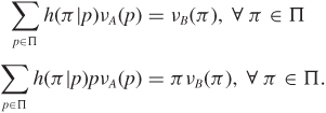
In other words, if forecaster A makes a prediction p, we can generate B’s prediction frequencies by utilizing the conditional distribution h(π|p).

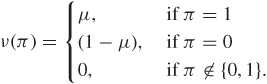
Let us go back to the forecaster that always announces the overall average, that is

We need to assume that μ ∊ Π—not so realistic if predictions are highly discrete, but convenient. This forecaster is the least refined forecaster. Alternatively, we say the forecaster exhibits zero sharpness. Any other forecaster is at least as refined as the least refined forecaster because we can set up the following stochastic transformation:

and apply Definition 10.5.

At another extreme of the spectrum of well-calibrated forecasters is the forecaster whose prediction each day is either 0 or 1:

Because this forecaster is well calibrated, his or her predictions have to also be always correct. This is the most refined forecaster is said to have has perfect sharpness. To see this, consider any other forecaster B, and use Definition 10.5 with the stochastic transformation

DeGroot and Fienberg (1982, p. 302) provide a result that simplifies the construction of useful stochastic transformations.

Theorem 10.2 Consider two well-calibrated forecasters A and B. Then A is at least as refined as B if and only if

where J is the number of elements in Π and π_(i) is the ith smallest element of Π.

DeGroot and Fienberg (1982) present a more general result that compares forecasters who are not necessarily well calibrated using the concept of sufficiency as introduced by Blackwell (1951) and Blackwell (1953).

At this point we are finally ready to explore the relationship between proper scoring rules and the concepts of calibration and refinement. Let us go back to the quadratic scoring rule, or Brier score, which in the setting of this section is

This score can be rewritten as

The first summation on the right hand side of the above equation measures the distance between the forecasts and the relative frequency of rainy days; that is, it is a measure of the calibration of the forecaster. This component is zero if the forecast is well calibrated. The second summation term is a measure of the refinement of the forecaster and it shows that the score is improved with values of close to 0 or 1. It can be approximately interpreted as a weighted average of the binspecific conditional variances, where bins are defined by the common forecast π. This decomposition illustrates how the squared error loss combines elements of calibration and forecasting, and is the counterpart of the bias/variance decomposition we have seen in equation (7.19) with regard to parameter estimation under squared error loss.

DeGroot and Fienberg (1983) generalize this beyond squared error loss: suppose that the forecaster’s subjective prediction is π and that he or she is scored on the basis of a strictly proper scoring rule specified by functions s₁ and s₂, which are, respectively, decreasing and increasing functions of π. The forecaster’s score is s₁(π) if it rains and s₂(π) otherwise. The next theorem tells us that strictly proper scoring rules can be partitioned into calibration and refinement terms.

Theorem 10.3 Suppose that the forecaster’s predictions are characterized by functions and ν(π) with a strictly proper scoring rule specified by functions s₁(π) and s₂(π). The forecaster’s overall score is S which can be decomposed as S = S₁+S₂ where

with φ(p) = ps₁(p) + (1 – p)s₂(p), 0 ≤ p ≤ 1, a strictly convex function.

Note that in the above decomposition, S₁ is a measure of the forecaster’s calibration and achieves its minimum when ; that is, when the forecaster is well calibrated. On the other hand, S₂ is a measure of the forecaster’s refinement.

Although scoring rules can be used to compare probability assessments provided by competing forecasters, or models, in practice it is more common to separately assess calibration and refinement, or calibration and discrimination. Calibration is typically assessed by the bias term in BS, or the chi-square statistic built on the same two sets of frequencies. Discrimination is generally understood as the ability of a set of forecasts to separate rainy from dry days and is commonly quantified via the receiver operating characteristics (ROC) curve (Lusted 1971, McNeil et al. 1975). A ROC curve quantifies in general the ability of a quantitative or ordinal measurement and scores (possibly a probability) to classify an associate binary measurement.

For a biological example, consider a population of individuals, some of whom have a binary genetic marker x = 1 and some of whom do not. A forecaster, or prediction algorithm, gives you a measurement π that has cumulative distribution

conditional on the true marker status x. In a specific binary decision problem we may be able to derive a cutoff point π₀ on the forecast and decide to “declare positive” all individuals for whom π > π₀. This declaration will lead to true positives but also some false positives. The fraction of true positives among the high-probability group, or sensitivity, is

while the fraction of true negatives among the low-probability group, or specificity, is

Generally a higher cutoff will decrease the sensitivity and increase the specificity, similarly to what happens to the coordinates of the risk set as we vary the cutoff on the test statistic in Section 7.5.1.

The ROC curve is a graph of β(π₀) versus 1 – α(π₀) as we vary π₀. Formally the ROC curve is given by the equation

β = 1 – F₁[1 – F₀(1 – α)].

The overall discrimination of a classifier is often summarized across all possible cutoffs by computing the area under the ROC curve, which turns out to be equal to the probability that a randomly selected person with the genetic marker has a forecast that is greater than a randomly selected person without the marker.

The literature on measuring the quality of probability assessments and the utility of predictive assays in medicine is extensive. Pepe (2003) provides a broad overview. Issues with comparing multiple predictions are explored in Pencina et al. (2008). An interesting example of evaluating probabilistic prediction in the context of specific medical decisions is given by Gail (2008).

10.4.2 Are Bayesians well calibrated?

A coherent probability forecaster expects to be calibrated in the long run. Consider a similar setting to the previous section and suppose in addition that, subsequent to each forecast π_i, the forecaster receives feedback in the form of the outcome x_i of the predicted event. Assume that π_i+1 represents the posterior probability of rain given the prior history x₁, ..., x_i, that is

π_i+1 = π(x_i+1|x₁, ..., x_i).

One complication now is that we can no longer assume that the forecasts live in a discrete set. One way to proceed is to select a subset, or subsequence, of days—for example, all days with forecast in a given interval—and compare forecasts π_i with the proportion of rainy day in the subset. To formalize, let ε_i be the indicator for whether day i is included in the set. Define

to be the number of selected days within horizon k,

to be the relative frequency of rainy days within the subset, and

as the average forecast probability within the tested subsequence. In this setting we can define long-run calibration as follows:

Definition 10.6 Given a subsequence such that ε_i = 1 infinitely often, the forecaster is calibrated in the long run if

with probability 1.

The condition that ε_i = 1 infinitely often is required so we never run out of events to compare and we can take the limit. To satisfy it we need to be careful in constructing subsets using a condition that will keep coming up.

This is a good point to remind ourselves that, from the point of view of the forecaster, the expected value of the forecaster’s posterior is his or her prior. For example, at the beginning of the series

and likewise at any stage in the process. This follows from the law of total probability, as long as m is the marginal distribution that is implied by the forecaster’s likelihood and priors. So, as a corollary

E_xi[π_i+1|x_i] – π_i = 0,

a property that makes the sequence of forecasts a so-called martingale. So if the data are generated from the very same stochastic model that is used in the updating step (that is, Bayes’ rule) then the forecasts are expected to be stable. Of course this is a big if.

In our setting, a consequence of this is that in the long run, a coherent forecaster who updates probabilities according to a Bayes rule expects to be well calibrated almost surely in the long run. This can be formalized in various ways. Details of theorems and proofs are in Pratt (1962), Dawid (1982), and Seidenfeld (1985). The good side of this result is that any coherent forecaster is not only internally consistent, but also prepared to become consistent with evidence, at least with evidence of the type he or she expects will accumulate. For example, if the forecaster’s probabilities are based on a parametric model whose parameters are unknown and are assigned a prior distribution, then, in the long run, if the data are indeed generated by the postulated model, the forecaster will learn model parameters no matter what the initial prior was, as long as a positive mass was assigned to the correct value. Also, any two coherent forecasters that agree on the model will eventually give very similar predictions.

Seidenfeld points out that this is a disappointment for those who may have hoped for calibration to provide an additional criterion for restricting the possible range of coherent probability specifications:

We are referring here to expected calibration by one’s own model. In reality different forecasters will use different models and may never agree with each other or with evidence. Dawid is concerned by the challenge this poses to the foundations of Bayesian statistics:

Whether this is indeed an irrational conclusion is a matter of debate, some of which can be enjoyed in the comments to Dawid’s paper, as well as in his rejoinder.

Just as in our discussion of Savage’s “small worlds,” here we must keep in mind that the theory of rationality needs to be circumscribed to a small enough, reasonably realistic, microcosm, within which it is humanly possible to specify probabilities. For example, specifying a model for all possible future meteorological data in a broad sense, say including all new technological advances in measurement, climate change, and so forth, is beyond human possibility. So the “small world” may need to evolve with time, at the price of some reshaping of the probability model and a modicum of temporal incoherence. Morrie DeGroot used to say that he carried in his pocket an ε of probability for complete surprises. He was coherent up to that ε! His ε would come in handy in the event that a long-held model turned out not to be correct. Without it, or the willingness to understand coherence with some flexibility, we would be stuck for life with statistical models we choose here and now because they are useful, computable, or currently supported by a dominant scientific theory, but later become obsolete. How to learn statistical models from data, and how to try to do so rationally, is the matter of the next chapter.

10.5 Exercises

Problem 10.1 A forecaster must announce probabilities q = (q₁, ..., q_J) for the events θ₁, ..., θ_J. These events form a partition: that is, one and only one of them will occur. The forecaster will be scored based on the scoring rule

Here 1_i=j is 1 if i = j and 0 otherwise. Let π = (π₁, ..., π_J) represent the forecaster’s own probability for the events θ₁, ..., θ_J. Show that this scoring rule is not proper. That is, show that there exists a vector q ≠ π such that

Because you are looking for a counterexample, it is okay to consider a simplified version of the problem, for example by picking a small J.

Problem 10.2 Show directly that the scoring rule s(θ_j, q) = q_j is not proper. See Winkler (1969) for further discussion about the implications of this fact.

Problem 10.3 Suppose that θ₁ and θ₂ are indicators of disjoint events (that is, θ₁θ₂ = 0) and consider θ₃ = θ₁ + θ₂ as the indicator of the union event. You have to announce probabilities q_θ1, q_θ2, and q_θ1+θ2 to these events, respectively. You will be scored according to the quadratic scoring rule: s(θ₁, θ₂, θ₃, q_θ1, q_θ2, q_θ3) = (q_θ1 – θ₁)² + (q_θ2 – θ₂)² + (q_θ3 – θ₃)². Prove the additive law, that is q_θ3 = q_θ1 + q_θ2.

Hint: Calculate the scores for the occurrence of θ₁(1 – θ₂), (1 – θ₁)θ₂, and (1 – θ₁)(1 – θ₂).

Problem 10.4 Show that the area under the ROC curve is equal to the probability that a randomly selected person with the genetic marker has an assay that is greater than a randomly selected person without the marker.

Problem 10.5 Prove Equation (10.8).

Problem 10.6 Consider a sequence of independent binary events with probability of success 0.4 Evaluate the two terms in equation (10.8) for the following four forecasters:

Charles:	always says 0.4.
Mary:	randomly chooses between 0.3 and 0.5.
Qing:	says either 0.2 or 0.3; when he says 0.2 it never rains, when he says 0.3 it always rains.
Ana:	follows this table:

	Rain	No rain
π = 0.3	0.15	0.35
π = 0.5	0.25	0.25

Comment on the calibration and refinement of these forecasters.