11
SHORTCUTS AND APPROXIMATIONS

So far, we’ve spent a lot of time looking at how to compute efficiently, especially with regard to memory usage. But there’s one thing that’s better than computing efficiently, and that’s not computing at all. This chapter looks at two ways to avoid computing: taking shortcuts and approximating.
We think of computers as very exact and precise. But, as we saw in “Representing Real Numbers” on page 14, they really aren’t. We can write code to be as exact as we want. For example, the UNIX bc utility is an arbitrary precision calculator that’s perfect if you need lots of accuracy, but it’s not a very efficient approach because computer hardware doesn’t support arbitrary precision. This leads to the question, how close is good enough for a particular application? Effective use of computing resources means not doing more work than necessary. Calculating all the digits of π before using it is just not rational!
Table Lookup
Many times it’s simpler and faster to look something up in a table than to do a calculation. We’ll look at a few examples of this approach in the following subsections. Table lookup is similar to the loop-invariant optimization that was discussed in Chapter 8 in that if you’re going to use something a lot, it often makes sense to calculate it once in advance.
Conversion
Suppose we need to read a temperature sensor and display the result in tenths of a degree Celsius (°C). A clever hardware designer has given us a circuit that produces a voltage based on the measured temperature that we can read using an A/D converter (see “Analog-to-Digital Conversion” on page 162). The curve looks like Figure 11-1.
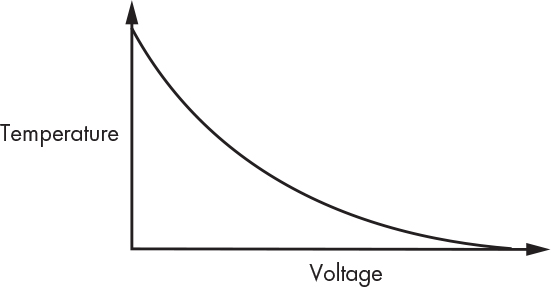
Figure 11-1: Temperature sensor curve
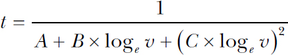
You can see that the curve is not a convenient straight line. We can calculate the temperature (t) from the voltage (v) using the following formula, where A, B, and C are constants determined by the particular model of sensor:
As you can see, a lot of floating-point arithmetic is involved, including natural logarithms, which is costly. So let’s skip it all. Instead, let’s build a table that maps voltage values into temperatures. Suppose we have a 10-bit A/D and that 8 bits is enough to hold our temperature value. That means we only need a 1,024-byte table to eliminate all the calculation, as shown in Figure 11-2.
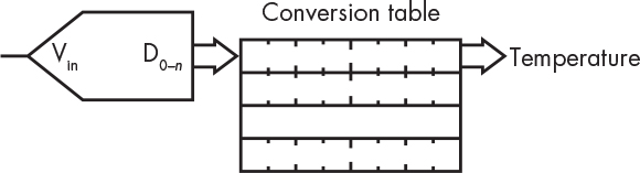
Figure 11-2: Table lookup conversion
Texture Mapping
Table lookup is a mainstay of texture mapping, a technique that helps provide realistic-looking images in video games and movies. The idea behind it is that pasting an image onto an object such as a wall takes a lot less computation than algorithmically generating all the detail. This is all well and good, but it has its own issues. Let’s say we have a brick wall texture such as the one in Figure 11-3.
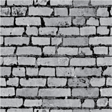
Figure 11-3: Brick wall texture
Looks pretty good. But video games aren’t static. You might be running away from a brick wall at high speed because you’re being chased by zombies. The appearance of the brick wall needs to change based on your distance from it. Figure 11-4 shows how the wall looks from a long distance away (on the left) and from very close (on the right).
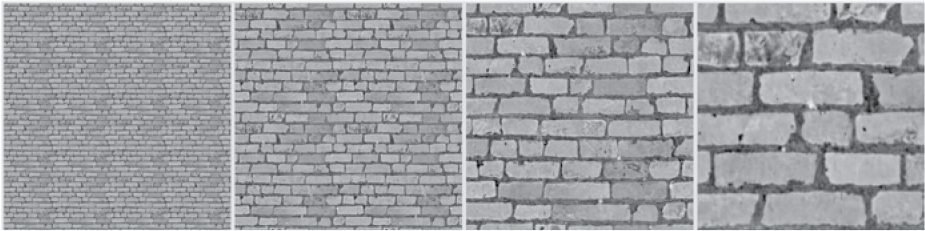
Figure 11-4: Brick wall texture at different distances
As you might expect, adjusting the texture for distance is a lot of work. As the viewpoint moves farther away from the texture, adjacent pixels must be averaged together. It’s important to be able to do this calculation quickly so that the image doesn’t jump around.
Lance Williams (1949–2017) at the New York Institute of Technology Graphics Language Laboratory devised a clever approach called MIP mapping (named from the Latin multum in parvo, meaning “many things in a small place”). His paper on this topic, entitled “Pyramidal Parametrics,” was published in the July 1983 SIGGRAPH proceedings. His method is still in use today, not only in software but also in hardware.
As we saw in “Representing Colors” on page 27, a pixel has three 8-bit components, one each for red, green, and blue. Williams noticed that on 32-bit systems, a quarter of the space was left over when these components were arranged in a rectangular fashion, as shown in Figure 11-5.
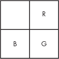
Figure 11-5: Color component arrangement with leftover space
He couldn’t just let that space go to waste, so he put it to good use in a different way than Tom Duff and Thomas Porter did (see “Adding Transparency” on page 29). Williams noticed that because it was one-fourth of the space, he could put a one-fourth-size copy of the image into that space, and then another one-fourth-size copy into that space, and so on, as shown in Figure 11-6. He called this arrangment a MIP map.
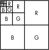
Figure 11-6: Multiple image layout
Making a MIP map out of our brick wall texture results in the image shown in Figure 11-7 (you’ll have to imagine the color components in this grayscale image).
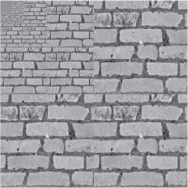
Figure 11-7: MIP mapped texture
As you can see, there’s a lot more detail in the closer-up images, where it’s important. This is interesting, but other than being a clever storage mechanism, what use is it? Take a look at Figure 11-8, which unfolds one of the colors of the MIP map into a pyramid.
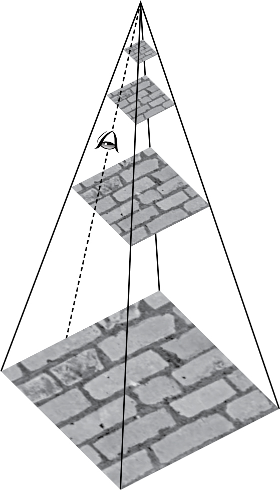
Figure 11-8: MIP map pyramid
The image at the tip of the pyramid is what things look like from far away, and there’s more detail as we head toward the base. When we need to compute the actual texture to display for the position of the eye in Figure 11-8, we don’t need to average together all the pixels in the base image; we just need to use the pixels in the nearest layer. This saves a lot of time, especially when the vantage point is far away.
Precomputing information that’s going to be used a lot—in this case, the lower-resolution versions of the texture—is equivalent to loop-invariant optimization.
Character Classification
Table lookup methods had a big influence on the addition of libraries to the programming language C. Back in Chapter 8, we saw that character classification—deciding which characters were letters, numbers, and so on—is an important part of lexical analysis. Going back to the ASCII code chart in Table 1-10, you could easily write code to implement classification, such as that shown in Listing 11-1.
int
isdigit(int c)
{
return (c >= '0' && c <= '9');
}
int
ishexdigit(int c)
{
return (c >= '0' && c <= '9' || c >= 'A' && c <= 'F' || c >= 'a' && c <= 'f');
}
int
isalpha(int c)
{
return (c >= 'A' && c <= 'Z' || c >= 'a' && c <= 'z');
}
int
isupper(int c)
{
return (c >= 'A' && c <= 'Z');
}
Listing 11-1: Character classification code
Some at Bell Labs suggested putting commonly useful functions, such as the ones in Listing 11-1, into libraries. Dennis Ritchie (1941–2011) argued that people could easily write their own. But Nils-Peter Nelson in the computer center had written an implementation of these routines that used a table instead of a collection of if statements. The table was indexed by character value, and each entry in the table had bits for aspects like uppercase, lowercase, digit, and so forth, as shown in Figure 11-9.
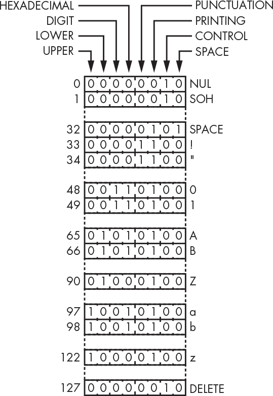
Figure 11-9: Character classification table
Classification, in this case, involved looking up the value in the table and checking the bits, as shown in Listing 11-2.
unsigned char table[128] = [ ... ];
#define isdigit(c) (table[(c) & 0x7f] & DIGIT)
#define ishexdigit(c) (table[(c) & 0x7f] & HEXADECIMAL)
#define isalpha(c) (table[(c) & 0x7f] & (UPPER | LOWER))
#define isupper(c) (table[(c) & 0x7f] & UPPER)
Listing 11-2: Table-driven character classification code
As you can see, the functions in Listing 11-2 are simpler than those in Listing 11-1. And they have another nice property, which is that they’re all essentially the same code; the only difference is the value of the constants that are ANDed with the table contents. This approach was 20 times faster than what anybody else had done, so Ritchie gave in and these functions were added as a library, setting the stage for additional libraries.
NOTE
You’ll notice that I use macros in Listing 11-2 but functions in Listing 11-1. In case you haven’t seen macros before, they’re a language construct that substitutes the code on the right for the code on the left. So, if your source code included isupper('a'), the language preprocessor would replace it with table[('a') & 0x7f] & UPPER. This is great for small chunks of code because there’s no function call overhead. But the code in Listing 11-1 couldn’t reasonably be implemented using macros because we have to handle the case where someone does isupper(*p++). If the code in Listing 11-1 were implemented as macros, then in ishexdigit, for example, p would be incremented six times, which would be a surprise to the caller. The version in Listing 11-2 references the argument only once, so that doesn’t happen.
Integer Methods
It should be obvious from the earlier discussion of hardware that some operations are cheaper to perform in terms of speed and power consumption than others. Integer addition and subtraction are inexpensive. Multiplication and division cost more, although we can multiply and divide by 2 cheaply using shift operations. Floating-point operations are considerably more expensive. Complex floating-point operations, such as the calculation of trigonometric and logarithmic functions, are much more expensive. In keeping with the theme for this chapter, it would be best if we could find ways to avoid using the more expensive operations.
Let’s look at some visual examples. Listing 11-3 modifies the web page skeleton from Listing 10-1 to have style, a script fragment, and a body.
1 <style>
2 canvas {
3 border: 5px solid black;
4 }
5 </style>
6 ...
7 <script>
8 $(function() {
9 var canvas = $('canvas')[0].getContext('2d');
10
11 // Get the canvas width and height. Force them to be numbers
12 // because attr yields strings and JavaScript often produces
13 // unexpected results when using strings as numbers.
14
15 var height = Number($('canvas').attr('height'));
16 var width = Number($('canvas').attr('width'));
17
18 canvas.translate(0, height);
19 canvas.scale(1, -1);
20 });
21 </script>
22 ...
23 <body>
24 <canvas width="500" height="500"></canvas>
25 </body>
Listing 11-3: Basic canvas
I briefly mentioned canvases back in “HTML5” on page 255. A canvas is an element on which you can do free-form drawing. You can think of it as a piece of graph paper.
The canvas “graph paper” isn’t exactly what you’re used to because it doesn’t use the standard Cartesian coordinate system by default. This is an artifact of the direction in which the raster was drawn on televisions (see “Raster Graphics” on page 180); the raster starts at the upper left. The x-coordinate behaves normally, but the y-coordinate starts at the top and increases downward. This coordinate system was kept when television monitors were repurposed for computer graphics.
Modern computer graphics systems support arbitrary coordinate systems for which graphics hardware often includes support. A transformation is applied to every (x, y) coordinate you specify and maps your coordinates to the screen coordinates (x′, y′) using the following formulas:
x′ = Ax + By + C
y′ = Dx + Ey + F
The C and F terms provide translation, which means they move things around. The A and E terms provide scaling, which means they make things bigger and smaller. The B and D terms provide rotation, which means they change the orientation. These are often represented in matrix form.
For now, we just care about translation and scaling to convert the canvas coordinate system into a familiar one. We translate downward by the height of the canvas on line 13 and then flip the direction of the y-axis on line 14. The order matters; if we did these translations in the reverse order, the origin would be above the canvas.
Graphics are effectively created from blobs of primary colors plopped on a piece of graph paper (see “Representing Colors” on page 27). But how fine a piece of graph paper do we need? And how much control do we need over the color blob composition?
The width and height attributes on line 19 set the size of the canvas in pixels (see “Digital Images” on page 173). The resolution of the display is the number of pixels per inch (or per centimeter). The size of the canvas on your screen depends on the resolution of your screen. Unless it’s a real antique, you probably can’t see the individual pixels. (Note that the resolution of the human eye isn’t a constant across the field of vision; see “A Photon Accurate Model of the Human Eye,” Michael Deering, SIGGRAPH 2005.) Even though current UHD monitors are awesome, techniques such as supersampling are still needed to make things look really good.
We’ll start by drawing things at a very low resolution so we can see the details. Let’s make some graph paper by adding a JavaScript function that clears the canvas and draws a grid, as shown in Listing 11-4. We’ll also use a scaling transformation to get integer value grid intersections. The scale applies to everything drawn on the canvas, so we have to make the line width smaller.
1 var grid = 25; // 25 pixel grid spacing
2
3 canvas.scale(grid, grid);
4 width = width / grid;
5 height = height / grid;
6 canvas.lineWidth = canvas.lineWidth / grid;
7 canvas.strokeStyle = "rgb(0, 0, 0)"; // black
8
9 function
10 clear_and_draw_grid()
11 {
12 canvas.clearRect(0, 0, width, height); // erase canvas
13 canvas.save(); // save canvas settings
14 canvas.setLineDash([0.1, 0.1]); // dashed line
15 canvas.strokeStyle = "rgb(128, 128, 128)"; // gray
16 canvas.beginPath();
17
18 for (var i = 1; i < height; i++) { // horizontal lines
19 canvas.moveTo(0, i);
20 canvas.lineTo(height, i);
21 }
22
23 for (var i = 1; i < width; i++) { // vertical lines
24 canvas.moveTo(i, 0);
25 canvas.lineTo(i, width);
26 }
27
28 canvas.stroke();
29 canvas.restore(); // restore canvas settings
30 }
31
32 clear_and_draw_grid(); // call on start-up
Listing 11-4: Drawing a grid
Straight Lines
Now let’s draw a couple of lines by placing colored circles on the grid in Listing 11-5. One line is horizontal, and the other has a slope of 45 degrees. The diagonal line blobs are slightly bigger so we can see both lines at the point where they intersect.
1 for (var i = 0; i <= width; i++) {
2 canvas.beginPath();
3 canvas.fillStyle = "rgb(255, 255, 0)"; // yellow
4 canvas.arc(i, i, 0.25, 0, 2 * Math.PI, 0);
5 canvas.fill();
6
7 canvas.beginPath();
8 canvas.fillStyle = "rgb(255, 0, 0)"; // red
9 canvas.arc(i, 10, 0.2, 0, 2 * Math.PI, 0);
10 canvas.fill();
11 }
Listing 11-5: Horizontal and diagonal lines
As you can see in Figure 11-10 and by running the program, the pixels are farther apart on the diagonal line than they are on the horizontal line (![]() farther apart, according to Pythagoras). Why does this matter? Because both lines have the same number of pixels emitting light, but when the pixels are farther apart on the diagonal line, the light density is less, making it appear dimmer than the horizontal line. There’s not much you can do about it; designers of displays adjust the shape of the pixels to minimize this effect. It’s more of an issue on cheaper displays than on desktop monitors and phones.
farther apart, according to Pythagoras). Why does this matter? Because both lines have the same number of pixels emitting light, but when the pixels are farther apart on the diagonal line, the light density is less, making it appear dimmer than the horizontal line. There’s not much you can do about it; designers of displays adjust the shape of the pixels to minimize this effect. It’s more of an issue on cheaper displays than on desktop monitors and phones.
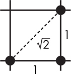
Figure 11-10: Pixel spacing
The horizontal, vertical, and diagonal lines are the easy cases. How do we decide what pixels to illuminate for other lines? Let’s make a line-drawing program. We’ll start by adding some controls after the canvas element in the body, as shown in Listing 11-6.
1 <div>
2 <label for="y">Y Coordinate: </label>
3 <input type="text" size="3" id="y"/>
4 <button id="draw">Draw</button>
5 <button id="erase">Erase</button>
6 </div>
Listing 11-6: Basic line-drawing program body
Then, in Listing 11-7, we’ll replace the code from Listing 11-5 with event handlers for the draw and erase buttons. The draw function uses the dreaded y = mx + b, with b always being 0 in our case. Surprise! Some stuff from math is actually used.
1 $('#draw').click(function() {
2 if ($('#y').val() < 0 || $('#y').val() > height) {
3 alert('y value must be between 0 and ' + height);
4 }
5 else if (parseInt($('#y').val()) != $('#y').val()) {
6 alert('y value must be an integer');
7 }
8 else {
9 canvas.beginPath(); // draw ideal line
10 canvas.moveTo(0, 0);
11 canvas.setLineDash([0.2, 0.2]); // dashed line
12 canvas.lineTo(width, $('#y').val());
13 canvas.stroke();
14
15 var m = $('#y').val() / width; // slope
16
17 canvas.fillStyle = "rgb(0, 0, 0)";
18
19 for (var x = 0; x <= width; x++) { // draw dots on grid
20 canvas.beginPath();
21 canvas.arc(x, Math.round(x * m), 0.15, 0, 2 * Math.PI, 0);
22 canvas.fill();
23 }
24
25 $('#y').val(''); // clear y value field
26 }
27 });
28
29 $('#erase').click(function() {
30 clear_and_draw_grid();
31 });
Listing 11-7: Floating-point line-drawing and erase functions
Let’s try this with a y-coordinate of 15. The result should look like Figure 11-11.
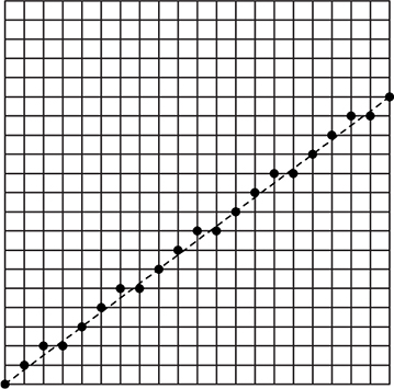
Figure 11-11: Line drawn using floating-point arithmetic
This looks pretty bad, but if you stand way back, it looks like a line. It’s as close as we can get. This is not just a computer graphics problem, as anyone who does cross-stitching can tell you.
Although the program we just wrote works fine, it’s not very efficient. It’s performing floating-point multiplication and rounding at every point. That’s at least an order of magnitude slower than integer arithmetic, even on modern machines. We do get some performance from computing the slope once in advance (line 15). It’s a loop invariant, so there’s a good chance that an optimizer (see “Optimization” on page 234) would do this for you automatically.
Way back in 1962, when floating-point was cost-prohibitive, Jack Bresenham at IBM came up with a clever way to draw lines without using floating-point arithmetic. Bresenham brought his innovation to the IBM patent office, which didn’t see the value in it and declined to pursue a patent. Good thing, since it turned out to be a fundamental computer graphics algorithm, and the lack of a patent meant that everybody could use it. Bresenham recognized that the line-drawing problem could be approached incrementally. Because we’re calculating y at each successive x, we can just add the slope (line 9 in Listing 11-8) each time through, which eliminates the multiplication. That’s not something an optimizer is likely to catch; it’s essentially a complex strength-reduction.
1 var y = 0;
2
3 canvas.fillStyle = "rgb(0, 0, 0)";
4
5 for (var x = 0; x <= width; x++) { // draw dots on grid
6 canvas.beginPath();
7 canvas.arc(x, Math.round(y), 0.15, 0, 2 * Math.PI, 0);
8 canvas.fill();
9 y = y + m;
10 }
Listing 11-8: Incrementally calculating y
We need floating-point arithmetic because the slope ![]() is a fraction. But the division can be replaced with addition and subtraction. We can have a decision variable d and add Δy on each iteration. The y value is incremented whenever d ≥ Δx, and then we subtract Δx from d.
is a fraction. But the division can be replaced with addition and subtraction. We can have a decision variable d and add Δy on each iteration. The y value is incremented whenever d ≥ Δx, and then we subtract Δx from d.
There is one last issue: rounding. We want to choose points in the middle of pixels, not at the bottom of them. That’s easy to handle by setting the initial value of d to ½m instead of 0. But we don’t want to introduce a fraction. No problem: we’ll just get rid of the ½ by multiplying it and everything else by 2 using 2Δy and 2Δx instead.
Replace the code that draws the dots on the grid with Listing 11-9’s “integer-only” version (we have no control over whether JavaScript uses integers internally, unlike in a language like C). Note that this code works only for lines with slopes in the range of 0 to 1. I’ll leave making it work for all slopes as an exercise for you.
1 var dx = width;
2 var dy = $('#y').val();
3 var d = 2 * dy - dx;
4 var y = 0;
5
6 dx *= 2;
7 dy *= 2;
8
9 canvas.fillStyle = "rgb(255, 255, 0)";
10 canvas.setLineDash([0,0]);
11
12 for (var x = 0; x <= width; x++) {
13 canvas.beginPath();
14 canvas.arc(x, y, 0.4, 0, 2 * Math.PI, 0);
15 canvas.stroke();
16
17 if (d >= 0) {
18 y++;
19 d -= dx;
20 }
21 d += dy;
22 }
Listing 11-9: Integer line drawing
One interesting question that arises from Listing 11-9 is, why isn’t the decision arithmetic written as shown in Listing 11-10?
1 var dy_minus_dx = dy - dx;
2
3 if (d >= 0) {
4 y++;
5 d -= dy_minus_dx;
6 }
7 else {
8 d += dy;
9 }
Listing 11-10: Alternate decision code
At first glance, this approach seems better because there’s only one addition to the decision variable per iteration. Listing 11-11 shows how this might appear in some hypothetical assembly language such as the one from Chapter 4.
load d load d
cmp #0 cmp #0
blt a blt a
load y load y
add #1 add #1
store y store y
load d load d
sub dx_plus_dy sub dx
bra b
a: add dy a: add dy
store d store d
b: ... ...
Listing 11-11: Alternate decision code assembly language
Notice that the alternate version is one instruction longer than the original. And in most machines, integer addition takes the same amount of time as a branch. Thus, the code we thought would be better is actually one instruction time slower whenever we need to increment y.
The technique used in Bresenham’s line algorithm can be applied to a large variety of other problems. For example, you can produce a smoothly changing color gradient, such as that shown in Figure 11-12, by replacing y with a color value.
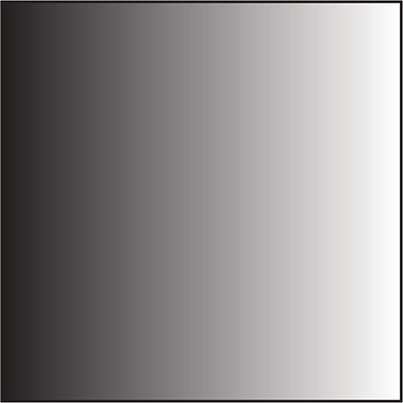
Figure 11-12: Color gradient
The gradient in Figure 11-12 was generated using the code shown in Listing 11-12 in the document ready function.
1 var canvas = $('canvas')[0].getContext('2d');
2 var width = $('canvas').attr('width');
3 var height = $('canvas').attr('height');
4
5 canvas.translate(0, height);
6 canvas.scale(1, -1);
7
8 var m = $('#y').val() / width;
9
10 var dx = width;
11 var dc = 255;
12 var d = 2 * dc - dx;
13 var color = 0;
14
15 for (var x = 0; x <= width; x++) {
16 canvas.beginPath();
17 canvas.strokeStyle = "rgb(" + color + "," + color + "," + color + ")";
18 canvas.moveTo(x, 0)
19 canvas.lineTo(x, height);
20 canvas.stroke();
21
22 if (d >= 0) {
23 color++;
24 d -= 2 * dx;
25 }
26 d += 2 * dc;
27 }
Listing 11-12: Color gradient code
Curves Ahead
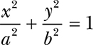
Integer methods aren’t limited to straight lines. Let’s draw an ellipse. We’ll stick to the simple case of ellipses whose axes are aligned with the coordinate axes and whose center is at the origin. They’re defined by the following equation, where a is one-half the width and b is one-half the height:
Assuming that we’re at the solid black point in Figure 11-13, we need to decide which of the three possible next points is closest to the ideal ellipse.
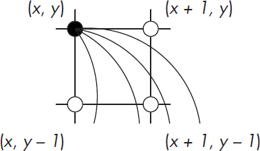
Figure 11-13: Ellipse decision points
Defining A = b2 and B = a2, we can rearrange the ellipse equation as Ax2 + By2 – AB = 0. We won’t be able to satisfy this equation most of the time because the points we need to draw on the integer grid aren’t likely to be the same as those on the ideal ellipse. When we’re at (x, y), we want to choose our next point to be the one in which Ax2 + By2 – AB is closest to 0. And we’d like to be able to do it without the seven multiplications in that equation.
Our approach is to calculate the value of the equation at each of the three possible points and then choose the point where the equation value is closest to 0. In other words, we’ll calculate a distance variable d at each of the three points using d = Ax2 + By2 – AB.
Let’s start by figuring out how to calculate d at the point (x + 1, y) without the multiplications. We can plug (x + 1) into the equation for x, as follows:
dx+1 = A(x + 1)2 + By2 – AB
Of course, squaring something is just multiplying it by itself:
dx+1 = A(x + 1)(x + 1) + By2 – AB
Multiplying it all out, we get:
dx+1 = x2 + 2Ax + A + By2 – AB
Now, if we subtract that from the original equation, we see that the difference between the equation at x and x + 1 is:
dx = 2Ax + A
We can add dx to d to get dx + 1. That doesn’t quite get us where we want to be, though, because there’s still a multiplication. So let’s evaluate dx at x + 1:
dxx+1 = 2A(x + 1) + A
dxx+1 = 2Ax + 2A + A
Just like before, subtraction gives us:
d2x = 2A
This yields a constant, which makes it easy to calculate d at (x + 1, y) without multiplication by using the intermediates dx and d2x:
2Ax+1 = 2Ax + d2x
That gets us the horizontal direction—the vertical is almost identical, except there’s a sign difference since we’re going in the –y direction:
dy = –2By + B
d2y = 2B
Now that we have all these terms, deciding which of the three points is closest to the ideal curve is simple. We calculate the horizontal difference dh to point (x + 1, y), the vertical difference dv to the point (x, y – 1), and the diagonal difference dd to the point (x + 1, y – 1) and choose the smallest. Note that although dx is always positive, dv and dd can be negative, so we need to take their absolute value before comparing, as shown in Figure 11-14.
Our ellipse-drawing algorithm draws the ellipse only in the first quadrant. That’s okay because there’s another trick that we can use: symmetry. We know that each quadrant of the ellipse looks the same as the first; it’s just flipped horizontally, vertically, or both. We could draw the whole ellipse by drawing (–x, y), (–x, –y), and (x, –y) in addition to drawing (x, y). Note that we could use eight-way symmetry if we were drawing circles.
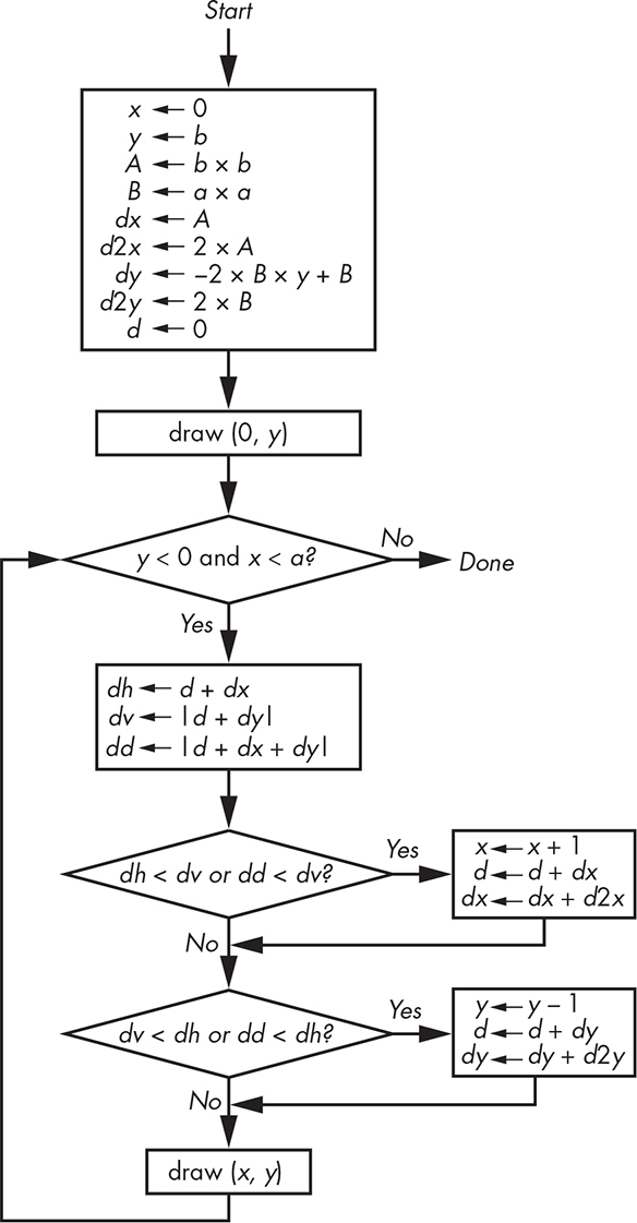
Figure 11-14: Ellipse-drawing algorithm
This algorithm includes some comparisons that could be simplified, which result from drawing one-quarter of the ellipse. The one-quarter ellipse could be partitioned into two sections at the point where the slope of the curve is 1. By doing so, we’d have one piece of code that only had to decide between horizontal and diagonal movements and another that had to decide between vertical and diagonal movements. Which one got executed first would depend on the values of a and b. But a lot more time is spent inside the loop making decisions than in the setup, so it’s a good trade-off.
The preceding algorithm has one serious deficiency: because it starts from the half-width (a) and half-height (b), it can draw only ellipses that are odd numbers of pixels in width and height, since the result is 2a wide and 2b high plus 1 for the axes.
Polynomials
The method we used to draw ellipses by incrementally calculating differences doesn’t scale well beyond conic sections (squared things). That’s because higher-order equations can do strange things, such as change direction several times within the space of a single pixel—which is pretty hard to test for efficiently.
But incrementally calculating differences can be generalized to any polynomials of the form y = Ax0 + Bx1 + Cx2 + . . . Dxn. All we have to do is generate n sets of differences so that we start our accumulated additions with a constant. This works because, unlike with the ellipse-drawing code, the polynomials have only a single independent variable. You may remember Charles Babbage’s difference engine from “The Case for Digital Computers” on page 34. It was designed to do just this: evaluate equations using incremental differences.
Recursive Subdivision
We touched briefly on recursive subdivision back in “Stacks” on page 122. It’s a technique with many uses. In this section, we’ll examine how to use it to get by with the minimum amount of work.
Spirals
Our line-drawing code can be leveraged for more complicated curves. We can calculate some points and connect them together using lines.
Your math class has probably covered the measurement of angles in degrees, so you know that there are 360 degrees in a circle. You may not be aware that there are other systems of measurement. A commonly used one is radians. There are 2π radians in a circle. So 360 degrees is 2π radians, 180 degrees is π radians, 90 degrees is π/2 radians, 45 degrees is π/4 radians, and so on. You need to know this because many trigonometric functions available in math libraries, such as the ones in JavaScript, expect angles in radians instead of degrees.
We’ll use curves drawn in polar coordinates for our examples because they’re pretty. Just in case you haven’t learned this yet, polar coordinates use radius r and angle θ instead of x and y. Conversion to Cartesian coordinates is easy: x = rcosθ and y = rsinθ. Our first example draws a spiral using r = θ × 10; the point that we draw gets farther away from the center as we sweep through the angles. We’ll make the input in degrees because it’s not as intuitive for many people to think in radians. Listing 11-13 shows the body for the controls.
<canvas width="500" height="500"></canvas>
<div>
<label for="degrees">Degrees: </label>
<input type="text" size="3" id="degrees"/>
<button id="draw">Draw</button>
<button id="erase">Erase</button>
</div>
Listing 11-13: Spiral body
We’ll skip the grid here because we need to draw more detail. Because we’re doing polar coordinates, Listing 11-14 puts (0, 0) at the center.
canvas.scale(1, -1);
canvas.translate(width / 2, -height / 2);
$('#erase').click(function() {
canvas.clearRect(-width, -height, width * 2, height * 2);
});
$('#draw').click(function() {
if (parseFloat($('#degrees').val()) == 0)
alert('Degrees must be greater than 0');
else {
for (var angle = 0; angle < 4 * 360; angle += parseFloat($('#degrees').val())) {
var theta = 2 * Math.PI * angle / 360;
var r = theta * 10;
canvas.beginPath();
canvas.arc(r * Math.cos(theta), r * Math.sin(theta), 3, 0, 2 * Math.PI, 0);
canvas.fill();
}
}
});
Listing 11-14: Dotted spiral JavaScript
Enter a value of 10 for degrees and click Draw. You should see something like Figure 11-15.
Notice that the dots get farther apart as we get farther from the origin, even though they overlap near the center. We could make the value of degrees small enough that we’d get a good-looking curve, but that means we’d have a lot of points that overlap, which is a lot slower, and it’s difficult to guess the value needed for an arbitrary function.
Let’s try drawing lines between the points. Swap in Listing 11-15 for the drawing code.
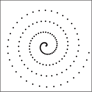
Figure 11-15: Dotted spiral
canvas.beginPath();
canvas.moveTo(0, 0);
for (var angle = 0; angle < 4 * 360; angle += parseFloat($('#degrees').val())) {
var theta = 2 * Math.PI * angle / 360;
var r = theta * 10;
canvas.lineTo(r * Math.cos(theta), r * Math.sin(theta));
}
canvas.stroke();
Listing 11-15: Spiral line JavaScript
Enter a value of 20 for degrees and click Draw. Figure 11-16 shows what you should see.
Not very pretty. Again, it looks good near the center but gets worse as we progress outward. We need some way to compute more points as needed—which is where our old friend recursive subdivision comes into play. We’re drawing lines using the spiral function between two angles, θ1 and θ2. What we’ll do is have some close enough criterion, and if a pair of points is not close enough, we’ll halve the difference in the angles and try again until we do get close enough. We’ll use the distance formula ![]() to find the distance between points, as shown in Listing 11-16.
to find the distance between points, as shown in Listing 11-16.
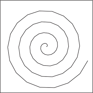
Figure 11-16: Spiral line
var close_enough = 10;
function
plot(theta_1, theta_2)
{
var r;
r = theta_1 * 10;
var x1 = r * Math.cos(theta_1);
var y1 = r * Math.sin(theta_1);
r = theta_2 * 10;
var x2 = r * Math.cos(theta_2);
var y2 = r * Math.sin(theta_2);
if (Math.sqrt(((x2 - x1) * (x2 - x1) + (y2 - y1) * (y2 - y1))) < close_enough) {
canvas.moveTo(x1, y1);
canvas.lineTo(x2, y2);
}
else {
plot(theta_1, theta_1 + (theta_2 - theta_1) / 2);
plot(theta_1 + (theta_2 - theta_1) / 2, theta_2);
}
}
$('#draw').click(function() {
if (parseFloat($('#degrees').val()) == 0)
alert('Degrees must be greater than 0');
else {
canvas.beginPath();
for (var angle = 0; angle < 4 * 360; angle += parseFloat($('#degrees').val())) {
var old_theta;
var theta = 2 * Math.PI * angle / 360;
if (angle > 0)
plot(old_theta, theta);
old_theta = theta;
}
}
canvas.stroke();
});
Listing 11-16: Recursive spiral line JavaScript
You’ll notice that as long as close_enough is small enough, the size of the increment in degrees doesn’t matter because the code automatically generates as many intermediate angles as needed. Play around with different values for close_enough; maybe add an input field so that it’s easy to do.
The determination of close enough is very important for certain applications. Though it’s beyond the scope of this book, think about curved objects that you’ve seen in movies. Shining light on them makes them look more realistic. Now imagine a mirrored sphere approximated by some number of flat faces just like the spiral was approximated by line segments. If the flat faces aren’t small enough, it turns into a disco ball (a set of flat surfaces approximating a sphere), which reflects light in a completely different manner.
Constructive Geometry
Chapter 5 briefly mentioned quadtrees and showed how they could represent shapes. They’re an obvious use of recursion because they’re a hierarchical mechanism for dividing up space.
We can perform Boolean operations on quadtrees. Let’s say we want to design something like the engine gasket in Figure 11-17.
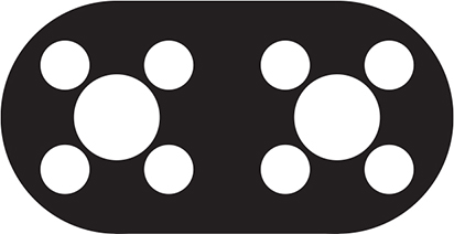
Figure 11-17: Engine gasket
We’ll need a data structure for a quadtree node, plus two special leaf values—one for 0, which we’re coloring white, and one for 1, which we’re coloring black. Figure 11-18 shows a structure and the data it represents. Each node can reference four other nodes, which is a good use for pointers in languages such as C.
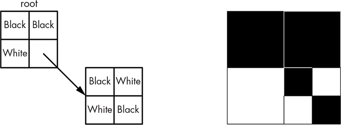
Figure 11-18: Quadtree node
We don’t need to keep track of the size of a node. All operations start from the root, the size of which is known, and each child node is one-quarter the size of its parent. Figure 11-19 shows us how to get the value at a location in the tree.
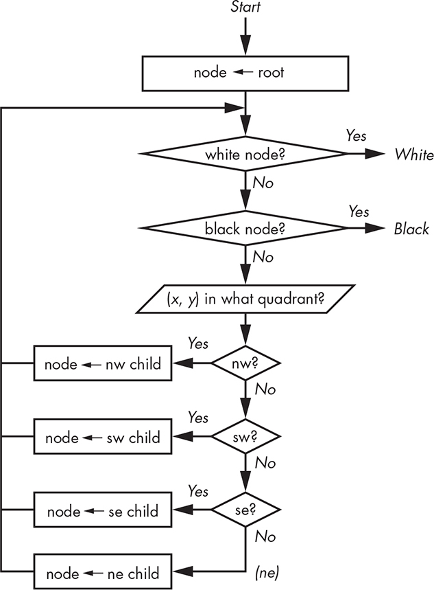
Figure 11-19: Get value of (x, y) coordinate in quadtree
Figure 11-20 shows how we would set the value of (that is, make black) an (x, y) coordinate in a quadtree. Note that “done” means “return from the function” since it’s recursive.
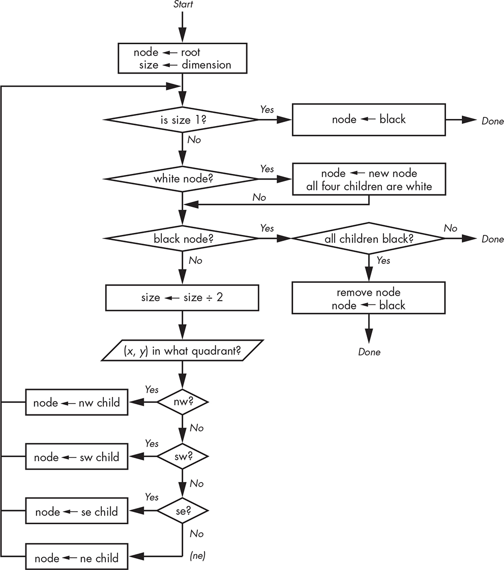
Figure 11-20: Set value of (x, y) coordinate in quadtree
This is similar to the value-getting code in Figure 11-19. At a high level, it descends the tree, subdividing as it goes, until it reaches the 1×1 square for the (x, y) coordinate and sets it to black. Any time it hits a white node, it replaces it with a new node having four white children so there’s a tree to keep descending. On the way back up, any nodes having all black children are replaced by a black node. This happens any time a node with three black children has the fourth set to black, as shown in Figure 11-21.
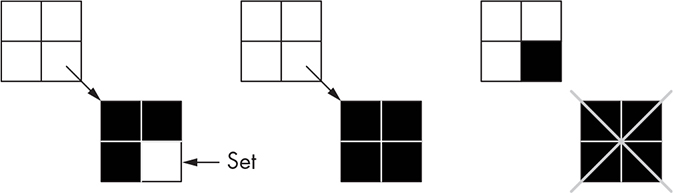
Figure 11-21: Coalescing a node
Coalescing nodes not only makes the tree take less memory, but it also makes many operations on the tree faster because it’s not as deep.
We need a way to clear (that is, make white) the value of an (x, y) coordinate in a quadtree. The answer is fairly similar to the setting algorithm. The differences are that we partition black nodes instead of white ones and we coalesce white nodes instead of black ones.
We can build some more complicated drawing functions on top of our value-setting function. It’s easy to draw rectangles by invoking the set function for each coordinate. We can do the same for ellipses using the algorithm from “Curves Ahead” on page 298 and symmetry.
Now for the fun stuff. Let’s create quadtree versions for some of our Boolean logic functions from Chapter 1. The NOT function is simple: just descend the tree and replace any black nodes with white ones and vice versa. The AND and OR functions in Figure 11-22 are more interesting. These algorithms aren’t designed to perform the equivalents of C = a AND b and C = a OR b. Instead, they implement dst &= src and dst |= src, as in the assignment operators found in many languages. The dst operand is the one modified.
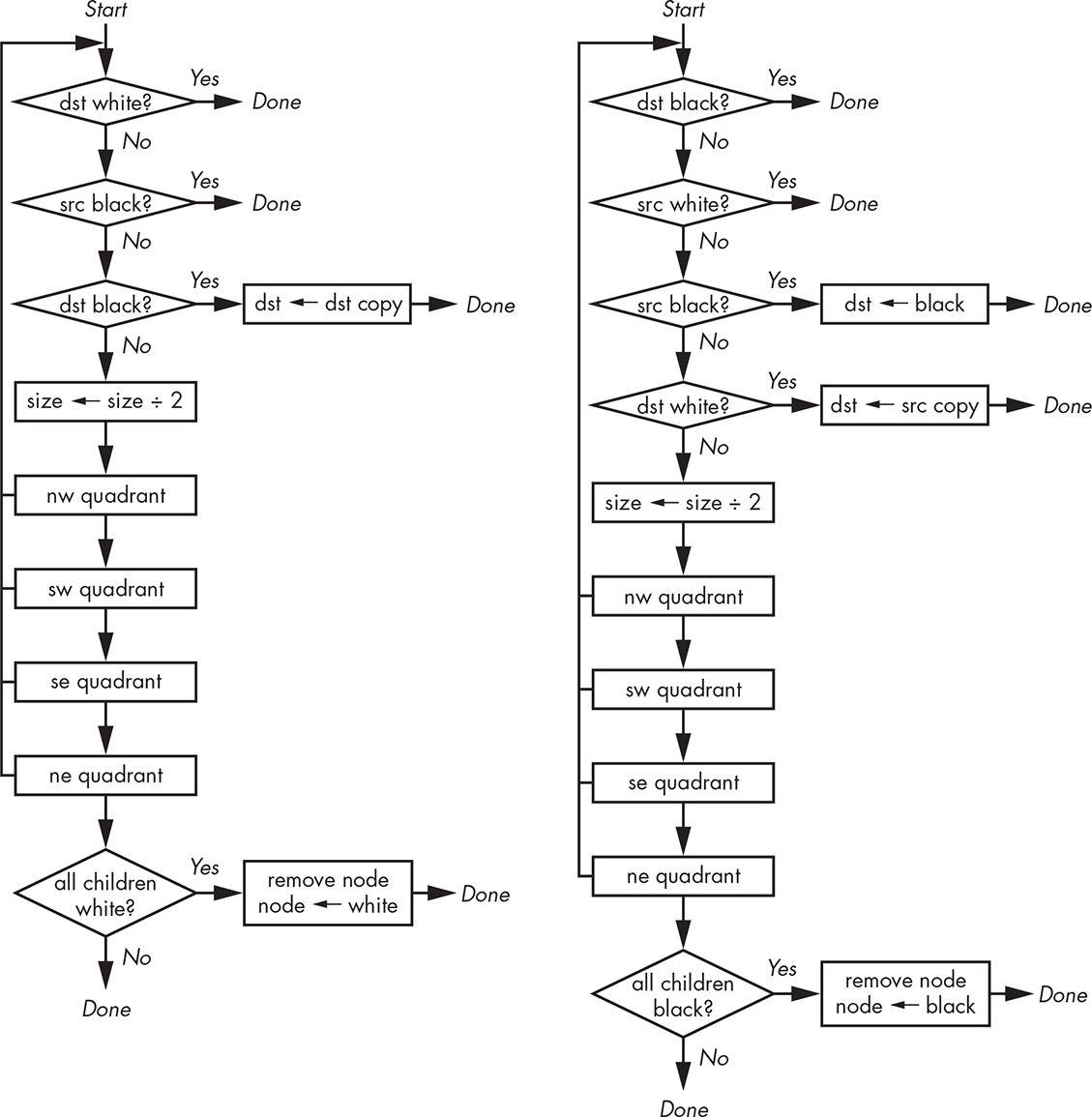
Figure 11-22: Quadtree AND and OR functions
Now that we have all these tools, let’s build our gasket. We’ll do it at low resolution so the details are visible. We’ll start with an empty gasket quadtree on the left and a scratch quadtree in the center in which we draw a big circle. The scratch quadtree is OR’d with the gasket, producing the result on the right as shown in Figure 11-23. Note how the coalescing keeps the number of subdivisions to a minimum.

Figure 11-23: Gasket, circle, circle OR gasket
Next we’ll make another circle in a different position and combine it with the partially completed gasket, as shown in Figure 11-24.
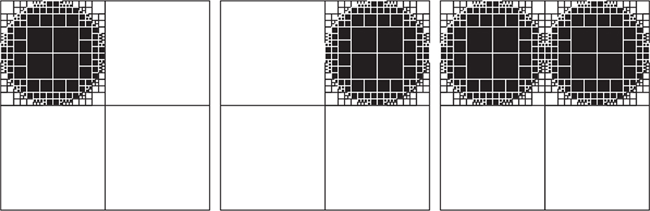
Figure 11-24: Adding to the gasket
Continuing on, we’ll make a black rectangle and combine it with the gasket, as shown in Figure 11-25.
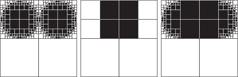
Figure 11-25: Adding the rectangle
The next step is to make a hole. This is accomplished by making a black circle and then inverting it using the NOT operation to make it white. The result is then ANDed with the partially completed gasket, resulting in the hole as seen in Figure 11-26.
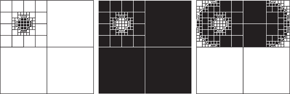
Figure 11-26: ANDing a NOT-hole
It’s getting boring at this point. We need to combine another hole, in the same way as shown in Figure 11-26, and then eight smaller holes in a similar fashion. You can see the result in Figure 11-27.

Figure 11-27: Completed gasket
As you can see, we can use Boolean functions on quadtrees to construct objects with complicated shapes out of simple geometric pieces. Although we used a two-dimensional gasket as our example, this is more commonly done in three dimensions. Twice as many nodes are needed for three dimensions, so the quadtree is extended into an octree, an example of which is shown in Figure 11-28.
Building complex objects in three dimensions using the preceding techniques is called constructive solid geometry. The three-dimensional counterpart to a two-dimensional pixel is called a voxel, which sort of means “volume pixel.”
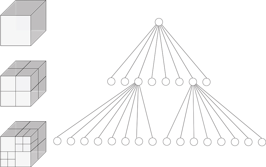
Figure 11-28: Octree
Octrees are a common storage method for CAT scan and MRI data. These machines generate a stack of 2D slices. It’s a simple matter to peel away layers to obtain cutaway views.
Shifting and Masking
One of the downsides of quadtrees is that the data is scattered around memory; they have terrible locality of reference. Just because two squares are next to each other in the tree doesn’t mean they’re anywhere near each other in memory. This becomes a problem when we have to convert data from one memory organization to another. We could always move data 1 bit at a time, but that would involve a large number of memory accesses—which we want to minimize, because they’re slow.
One task where this situation arises is displaying data. That’s because the display memory organization is determined by the hardware. As mentioned back in “Raster Graphics” on page 180, each row of the raster is painted one at a time in a particular order. A raster row is called a scan line. The whole collection of scan lines is called a frame buffer.
Let’s say we want to paint our completed gasket from Figure 11-27 on a display. For simplicity, we’ll use a monochrome display that has 1 bit for each pixel and uses 16-bit-wide memory. That means the upper-leftmost 16 pixels are in the first word, the next 16 are in the second, and so on.
The upper-left square in Figure 11-27 is 4×4 pixels in size and is white, which means we need to be clearing bits in the frame buffer. We’ll use the coordinates and size of the quadtree square to construct a mask, as shown in Figure 11-29.
Figure 11-29: AND mask
We can then AND this mask with all the affected rows, costing only two memory accesses per row: one for read and one for write. We would do something similar to set bits in the frame buffer; the mask would have 1s in the area to set, and we would OR instead of AND.
Another place where this comes into play is when drawing text characters. Most text characters are stored as bitmaps, two-dimensional arrays of bits, as shown in Figure 11-30. Character bitmaps are packed together to minimize memory use. That’s how text characters used to be provided; now they come as geometric descriptions. But for performance reasons, they’re often converted into bitmaps before use, and those bitmaps are usually cached on the assumption that characters get reused.
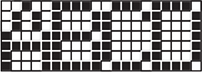
Figure 11-30: Bitmap text characters
Let’s replace the character B on the display shown in Figure 11-31 with a C.
Figure 11-31: Bitmap text characters
The C is located in bits 10 through 14 and needs to go into bits 6 through 10. For each row, we need to grab the C and then mask off everything else in the word. Then we need to shift it into the destination position. The destination must be read and the locations that we want to overwrite masked off before combining with the shifted C and being written, as shown in Figure 11-32.

Figure 11-32: Painting a character
This example uses three memory accesses per row: one to fetch the source, one to fetch the destination, and one to write the result. Doing this bit by bit would take five times that amount.
Keep in mind that there are often additional complications when the source or destination spans word boundaries.
More Math Avoidance
We discussed some simple ways to avoid expensive math in “Integer Methods” on page 290. Now that we have the background, let’s talk about a couple of more complicated math-avoidance techniques.
Power Series Approximations
Here’s another take on getting close enough. Let’s say we need to generate the sine function because we don’t have hardware that does it for us. One way to do this is with a Taylor series:
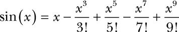
Figure 11-33 shows a sine wave and the Taylor series approximations for different numbers of terms. As you can see, the more terms, the closer the result is to an ideal sine.
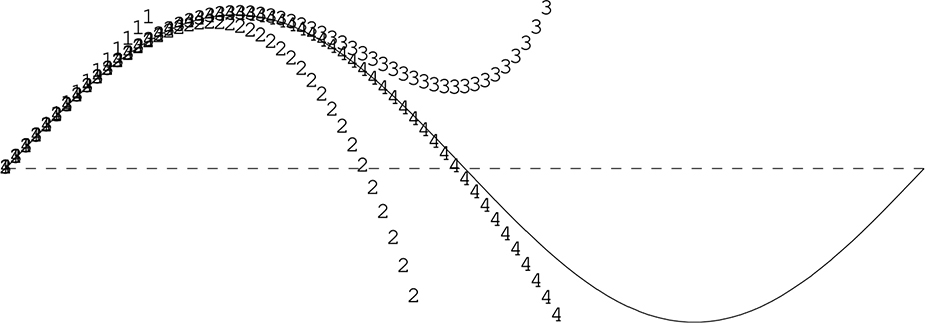
Figure 11-33: Taylor series for sine
It’s a simple matter to add terms until you get the desired degree of accuracy. It’s also worth noting that fewer terms are needed for angles more acute than 90 degrees, so you can be more efficient by using symmetry for other angles.
Note that we can reduce the number of multiplications required by initializing a product to x, precomputing –x2, and multiplying the product by –x2 to get each term. All the denominators are constants that could reside in a small table indexed by the exponent. Also, we don’t have to compute all of the terms. If we need only two digits of accuracy, we can stop when computing more terms doesn’t change those digits.
The CORDIC Algorithm
Jack Volder at Convair invented the Coordinate Rotation Digital Computer (CORDIC) algorithm in 1956. CORDIC was invented to replace an analog part of the B-58 bomber navigation system with something more accurate. CORDIC can be used to generate trigonometric and logarithmic functions using integer arithmetic. It was used in the HP-35, the first portable scientific calculator, released in 1972. It was also used in the Intel 80x87 family of floating-point coprocessors.
The basic idea of CORDIC is illustrated in Figure 11-34. Because it’s a unit circle (radius of 1) the x- and y-coordinates of the arrow ends are the cosine and sine of the angle. We want to rotate the arrow from its original position along the x-axis in smaller and smaller steps until we get to the desired angle and then grab the coordinates.
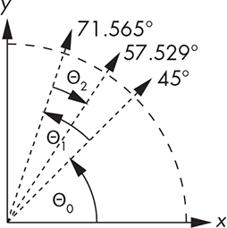
Figure 11-34: CORDIC algorithm overview
Let’s say we want sin(57.529°). As you can see, we first try 45 degrees, which isn’t enough, so we take another step of 25.565 degrees, getting us to 71.565 degrees, which is too much. We then go backward by 14.036 degrees, which gets us to our desired 57.529 degrees. We’re clearly performing some sort of subdivision but with weird values for the angles.
We saw the equations for transformation earlier in “Integer Methods,” where we cared only about translation and scaling. The CORDIC algorithm is based on rotation. The following equations, the general form of which you’ve seen, show us how (x, y) is rotated by angle θ to get a new set of coordinates (x′, y′):
x′ = x × cos(θ) – y × sin(θ)
y′ = x × sin(θ) + y × cos(θ)
Although this is mathematically correct, it seems useless because we wouldn’t be discussing an algorithm that generates sines and cosines if they were already available.
Let’s make it worse before making it better by rewriting the equations in terms of tangents using the trigonometric identity:
Because we’re dividing by cos(θ), we need to multiply the result by the same:
That looks pretty ugly. We’re making a bad situation worse, but that’s because we haven’t talked about the trick, which goes back to the weird angles. It turns out that tan(45°) = 1, tan(26.565°) = ½, and tan(14.036°) = ¼. That sure looks like some simple integer division by 2, or as Maxwell Smart might have said, “the old right shift trick.” It’s a binary search of the tangents of the angles.
Let’s see how this plays out for the example in Figure 11-34. There are three rotations that get us from the original coordinates to the final ones. Keep in mind that, per Figure 11-34, x0 = 1 and y0 = 0:

Note the sign change in the last set of equations that result from going the other (clockwise) direction; when we’re going clockwise, the sign of the tangent is negative. Plugging the equations for (x1, y1) into the equations for (x2, y2) and plugging that into the equations for (x3, y3) and then factoring out the cosines (and cleaning out the multiplications by 1) gives us the following:
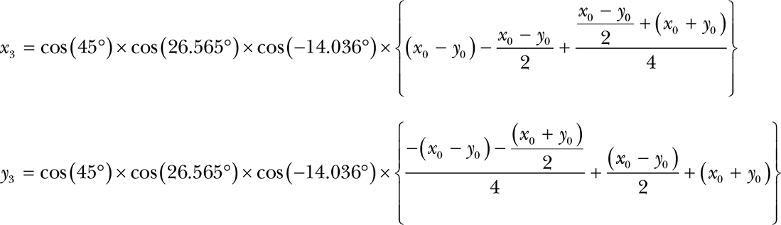
So what about those cosines? Skipping the mathematical proof, it turns out that as long as we have enough terms:
cos(45°) × cos(26.565°) × cos(–14.036°) × . . . = 0.607252935008881
That’s a constant, and we like constants. Let’s call it C. We could multiply it at the end like this:
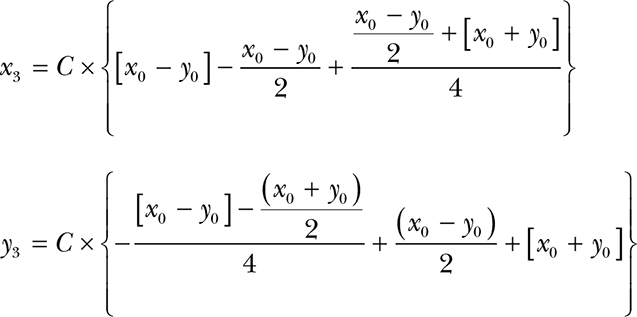
But we could save that multiplication by just using the constant for x0, as shown next. We’ll also eliminate y0, since it’s 0. It ends up looking like this:
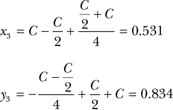
If you check, you’ll discover that the values for x3 and y3 are pretty close to the values of the cosine and sine of 57.529 degrees. And that’s with only three terms; more terms gets us closer. Notice that this is all accomplished with addition, subtraction, and division by 2.
Let’s turn this into a program that gives us a chance to introduce several additional tricks. First, we’ll use a slightly different version of CORDIC called vectoring mode; so far, we’ve been discussing rotation mode because it’s a little easier to understand. We’ve seen that in rotation mode we start with a vector (arrow) along the x-axis and rotate it until it’s at the desired angle. Vectoring mode is sort of the opposite; we start at our desired angle and rotate it until we end up with a vector along the x-axis (angle of 0). Doing it this way means we can just test the sign of the angle to determine the direction of rotation for a step; it saves a comparison between two numbers.
Second, we’re going to use table lookup. We’ll precompute a table of angles with tangents of 1, ½, ¼, and so on. We only need to do this once. The final algorithm is shown in Figure 11-35.
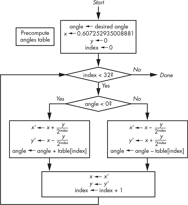
Figure 11-35: CORDIC flowchart
Now let’s write a C program that implements this algorithm using even more tricks. First, we’re going to express our angles in radians instead of in degrees.
The second trick is related to the first. You may have noticed that we haven’t encountered any numbers greater than 1. We can design our program to work in the first quadrant (between 0 and 90 degrees) and get the others using symmetry. An angle of 90 degrees is π/2, which is ≈ 1.57. Because we don’t have a wide range of numbers, we can use a fixed-point integer system instead of floating-point.
We’re going to base our sample implementation on 32-bit integers. Because we need a range of ≈ ±1.6, we can make bit 30 be the ones, bit 29 the halves, bit 28 the quarters, bit 27 the eighths, and so on. We’ll use the MSB (bit 31) as the sign bit. We can convert floating-point numbers (as long as they’re in range) to our fixed-point notation by multiplying by our version of 1, which is 0x40000000, and casting (converting) that into integers. Likewise, we can convert our results into floating-point by casting them as such and dividing by 0x40000000.
Listing 11-17 shows the code, which is quite simple.
1 const int angles[] = {
2 0x3243f6a8, 0x1dac6705, 0x0fadbafc, 0x07f56ea6, 0x03feab76, 0x01ffd55b, 0x00fffaaa, 0x007fff55,
3 0x003fffea, 0x001ffffd, 0x000fffff, 0x0007ffff, 0x0003ffff, 0x0001ffff, 0x0000ffff, 0x00007fff,
4 0x00003fff, 0x00001fff, 0x00000fff, 0x000007ff, 0x000003ff, 0x000001ff, 0x000000ff, 0x0000007f,
5 0x0000003f, 0x0000001f, 0x0000000f, 0x00000008, 0x00000004, 0x00000002, 0x00000001, 0x00000000
6 };
7
8 int angle = (desired_angle_in_degrees / 360 * 2 * 3.14159265358979323846) * 0x40000000;
9
10 int x = (int)(0.6072529350088812561694 * 0x40000000);
11 int y = 0;
12
13 for (int index = 0; index < 32; index++) {
14 int x_prime;
15 int y_prime;
16
17 if (angle < 0) {
18 x_prime = x + (y >> index);
19 y_prime = y - (x >> index);
20 angle += angles[index];
21 }
22 else {
23 x_prime = x - (y >> index);
24 y_prime = y + (x >> index);
25 angle -= angles[index];
26 }
27
28 x = x_prime;
29 y = y_prime;
30 }
Listing 11-17: CORDIC implementation in C
Implementing CORDIC uses many of the goodies in our growing bag of tricks: recursive subdivision, precomputation, table lookup, shifting for power-of-two division, integer fixed-point arithmetic, and symmetry.
Somewhat Random Things
It’s very difficult to do completely random things on computers because they have to generate random numbers based on some formula, and that makes it repeatable. That kind of “random” is good enough for most computing tasks though, except for cryptography, which we’ll discuss in Chapter 13. In this section, we’ll explore some approximations based on pseudorandomness. We’re choosing visual examples because they’re interesting and printable.
Space-Filling Curves
Italian mathematician Giuseppe Peano (1858–1932) came up with the first example of a space-filling curve in 1890. Three iterations of it are shown in Figure 11-36.
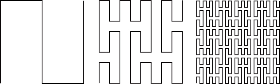
Figure 11-36: Peano curve
As you can see, the curve is a simple shape that is shrunk and repeated at different orientations. Each time that’s done, it fills more of the space.
Space-filling curves exhibit self-similarity, which means they look about the same both up close and far away. They’re a subset of something called fractals, which were popularized when Benoit Mandelbrot (1924–2010) published The Fractal Geometry of Nature (W. H. Freeman and Company, 1977). Many natural phenomena are self-similar; for example, a coastline has the same jaggedness when observed from a satellite and from a microscope.
The term fractal comes from fraction. Geometry includes numerous integer relationships. For example, doubling the length of the sides of a square quadruples its area. But an integer change in lengths in a fractal can change the area by a fractional amount, hence the name.
The Koch snowflake is an easy-to-generate curve first described in 1904 by Swedish mathematician Helge von Koch (1870–1924). It starts with an equilateral triangle. Each side is divided into thirds, and the center third is replaced by a triangle one-third of the size, with the edge in line with the original side omitted, as shown in Figure 11-37.
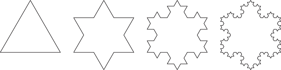
Figure 11-37: Four iterations of the Koch snowflake
You can see that complex and interesting shapes can be generated with a tiny amount of code and recursion. Let’s look at slightly more complex example: the Hilbert curve, first described in 1891 by German mathematician David Hilbert (1862–1943), as shown in Figure 11-38.
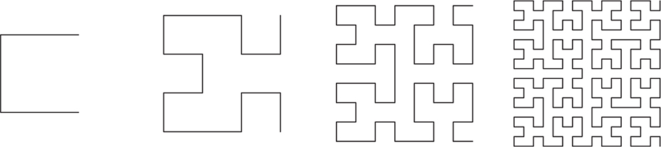
Figure 11-38: Four iterations of the Hilbert curve
The rules for the next iteration of the Hilbert curve are more complicated than for the Koch snowflake, because we don’t do the same thing everywhere. There are four different orientations of the “cup” shape that are replaced by smaller versions, as shown in Figure 11-39. There’s both a graphical representation and one using letters for right, up, left, and down. For each iteration, each corner of the shape on the left is replaced with the four shapes on the right (in order) at one-quarter the size of the shape on the left and then connected by straight lines.
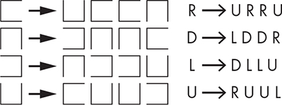
Figure 11-39: Hilbert curve rules
L-Systems
The rules in Figure 11-39 are similar to the regular expressions we saw back in “Regular Expressions” on page 224, but backward. Instead of defining what patterns are matched, these rules define what patterns can be produced. They’re called L-systems or Lindenmayer systems, after Hungarian botanist Aristid Lindenmayer (1925–1989), who developed them in 1968. Because they define what can be produced, they’re also called production grammars.
You can see from Figure 11-39 that replacing an R with the sequence U R R U transforms the leftmost curve in Figure 11-38 into the one next to it.
The nice thing about production grammars is that they’re compact and easy to both specify and implement. They can be used to model a lot of phenomena. This became quite the rage when Alvy Ray Smith at Lucasfilm published “Plants, Fractals, and Formal Languages” (SIGGRAPH, 1984); you couldn’t go outside without bumping into L-System-generated shrubbery. Lindenmayer’s work became the basis for much of the computer graphics now seen in movies.
Let’s make some trees so this book will be carbon-neutral. We have four symbols in our grammar, as shown in Listing 11-18.
E draw a line ending at a leaf
B draw a branch line
L save position and angle, turn left 45°
R restore position and angle, turn right 45°
Listing 11-18: Symbols for tree grammar
In Listing 11-19, we create a grammar that contains two rules.
B → B B
E → B L E R E
Listing 11-19: Tree grammar rules
You can think of the symbols and rules as a genetic code. Figure 11-40 shows several iterations of the grammar starting from E. Note that we’re not bothering to draw leaves on the ends of the branches. Also, beyond the first three, the set of symbols that define the tree are too long to show.
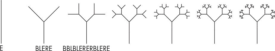
Figure 11-40: Simple L-system tree
As you can see, we get pretty good-looking trees without much work. L-systems are a great way to generate natural-looking objects.
Production grammars have been used to generate objects since long before computers. Knitting instructions are production grammars, for example, as shown in Listing 11-20.
k = knit
p = purl
s = slip first stitch purl wise
row1 → s p k k p p k k p p k p p k k p p k k p k k p p k k p p k p p k k p p k k p k
row2 → s k p p k k p p k k p k k p p k k p p k p p k k p p k k p k k p p k k p p k k
row5 → s p p k k p p k k p p p k k p p k k p p p k k p p k k p p p k k p p k k p p k
row6 → s k k p p k k p p k k k p p k k p p k k k p p k k p p k k k p p k k p p k k k
section → row1 row2 row1 row2 row5 row6 row5 row6 row2 row2 row2 row2 row6 row5 row6 row5
scarf → section ...
Listing 11-20: Production grammar for scarf in Figure 11-41
Executing the grammar in Listing 11-20 using the knitting needle I/O device for some number of sections yields a scarf, as shown in Figure 11-41.
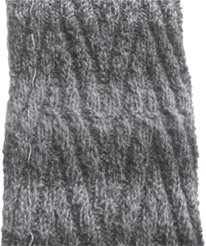
Figure 11-41: Scarf produced by production grammar
Going Stochastic
Stochastic is a good word to use when you want to sound sophisticated and random just won’t do. Alan Fournier and Don Fussell at the University of Texas at Dallas introduced the notion of adding randomness to computer graphics in 1980. A certain amount of randomness adds variety. For example, Figure 11-42 shows a stochastic modification of the L-system trees from the last section.
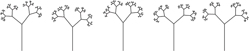
Figure 11-42: Stochastic L-system trees
As you can see, it generates a nice set of similar-looking trees. A forest looks more realistic when the trees aren’t all identical.
Loren Carpenter at Boeing published a paper that pioneered a simple way to generate fractals (“Computer Rendering of Fractal Curves and Surfaces,” SIGGRAPH, 1980). At SIGGRAPH 1983, Carpenter and Mandelbrot engaged in a very heated discussion about whether Carpenter’s results were actually fractals.
Carpenter left Boeing and continued his work at Lucasfilm. His fractal mountains produced the planet in Star Trek II: The Wrath of Khan. An interesting factoid is that the planet took about six months of computer time to generate. Because it was generated using random numbers, Spock’s coffin ended up flying through the side of the mountain for several frames. Artists had to manually cut a notch in the mountain to fix this.
Carpenter’s technique was simple. He randomly selected a point on a line and then moved that point a random amount. He recursively repeated this for the two line segments until things were close enough. It’s a bit like adding randomness to the Koch curve generator. Figure 11-43 shows a few random peaks.
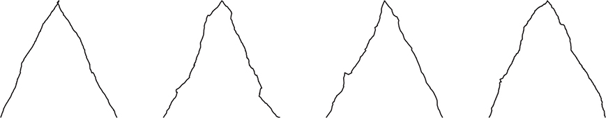
Figure 11-43: Fractal mountains
Once again, pretty good for not much work.
Quantization
Sometimes we don’t have a choice about approximating and must do the best we can. For example, we may have a color photograph that needs to be printed in a black-and-white newspaper. Let’s look at how we might make this transformation. We’ll use the grayscale image in Figure 11-44, since this book isn’t printed in color. Because it’s grayscale, each of the three color components is identical and in the range of 0 to 255.
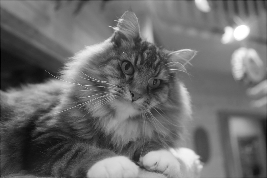
Figure 11-44: Tony Cat
We need to perform a process called quantization, which means taking the colors that we have available in the original image and assigning them to colors in the transformed image. It’s yet another sampling problem, as we have to take an analog (or more analog, in our case) signal and divide it among a fixed set of buckets. How do we map 256 values into 2?
Let’s start with a simple approach called thresholding. As you might guess from the name, we pick a threshold and assign anything brighter than that to white, and anything darker to black. Listing 11-21 makes anything greater than 127 white, and anything not white is black.
for (y = 0; y < height; y++)
for (x = 0; x < width; x++)
if (value_of_pixel_at(x, y) > 127)
draw_white_pixel_at(x, y);
else
draw_black_pixel_at(x, y);
Listing 11-21: Threshold pseudocode
Running this pseudocode on the image in Figure 11-44 produces the image in Figure 11-45.
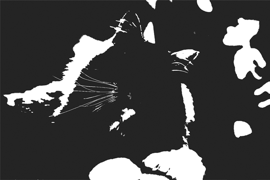
Figure 11-45: Threshold algorithm
That doesn’t look very good. But there’s not a lot we can do; we could monkey around with the threshold, but that would just give us different bad results. We’ll try to get better results using optical illusions.
British scientist Henry Talbot (1800–1877) invented halftone printing in the 1850s for just this reason; photography at the time was grayscale, and printing was black and white. Halftone printing broke the image up into dots of varying sizes, as shown in the magnified image on the left in Figure 11-46. As you can see on the right, your eye interprets this as shades of gray.
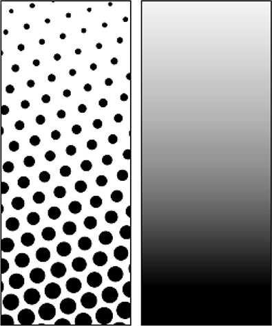
Figure 11-46: Halftone pattern
We can’t vary the dot size on a computer screen, but we want the same type of effect. Let’s explore some different ways to accomplish this. We can’t change the characteristics of a single dot that can be either black or white, so we need to adjust the surrounding dots somehow to come up with something that your eye will see as shades of gray. We’re effectively trading off image resolution for the perception of more shades or colors.
The name for this process is dithering, and it has an amusing origin going back once again to World War II analog computers. Someone noticed that the computers worked better aboard flying airplanes than on the ground. It turns out that the random vibration from the plane engines kept the gears, wheels, cogs, and such from sticking. Vibrating motors were subsequently added to the computers on the ground to make them work better by trembling them. This random vibration was called dither, based on the Middle English verb didderen, meaning “to tremble.” There are many dithering algorithms; we’ll examine only a few here.
The basic idea is to use a pattern of different thresholds for different pixels. In the mid-1970s, American scientist Bryce Bayer (1929–2012) at Eastman Kodak invented a key technology for digital cameras, the eponymous Bayer filter. The Bayer matrix is a variation that we can use for our purposes. Some examples are shown in Figure 11-47.
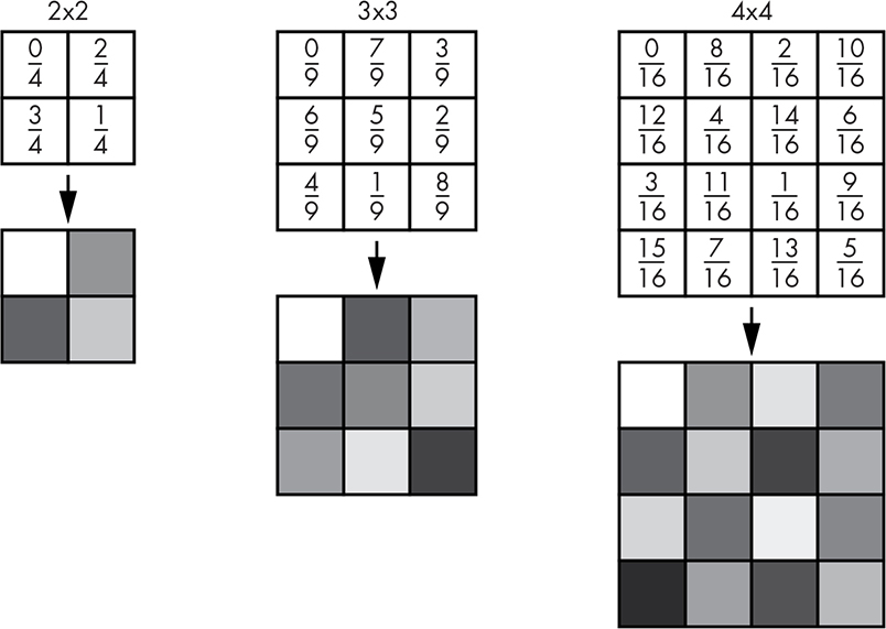
Figure 11-47: Bayer matrices
These matrices are tiled over the image, meaning they repeat in both the x and y directions, as shown in Figure 11-48. Dithering using tiled patterns is called ordered dithering, as there’s a predictable pattern based on position in the image.
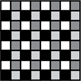
Figure 11-48: 2×2 Bayer matrix tiling pattern
Listing 11-22 shows the pseudocode for the Bayer matrices from Figure 11-47.
for (y = 0; y < height; y++)
for (x = 0; x < width; x++)
if (value_of_pixel_at(x, y) > bayer_matrix[y % matrix_size][x % matrix_size])
draw_white_pixel_at(x, y);
else
draw_black_pixel_at(x, y);
Listing 11-22: Bayer ordered dithering pseudocode
On to the important question: what does Tony Cat think of this? Figures 11-49 through 11-51 show him dithered using the three matrices just shown.
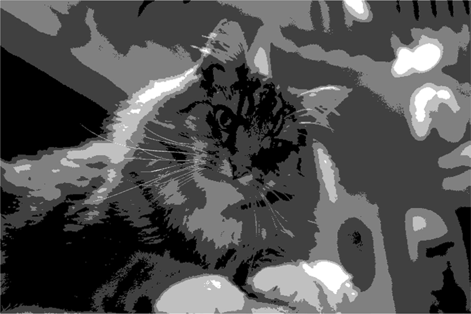
Figure 11-49: Tony dithered using the 2×2 Bayer matrix

Figure 11-50: Tony dithered using the 3×3 Bayer matrix

Figure 11-51: Tony dithered using the 4×4 Bayer matrix
As you can see, these are somewhat acceptable if you squint, and they improve with larger matrices. Not exactly the cat’s meow, but a lot better than thresholding. Doing more work by using larger matrices yields better results. But the tiling pattern shows through. Plus it can produce really trippy artifacts called moiré patterns for certain images. You might have seen these if you’ve ever grabbed a stack of window screens.
How can we eliminate some of these screening artifacts? Instead of using a pattern, let’s just compare each pixel to a random number using the pseudocode in Listing 11-23. The result is shown in Figure 11-52.
for (y = 0; y < height; y++)
for (x = 0; x < width; x++)
if (value_of_pixel_at(x, y) > random_number_between_0_and_255())
draw_white_pixel_at(x, y);
else
draw_black_pixel_at(x, y);
Listing 11-23: Random-number dithering pseudocode
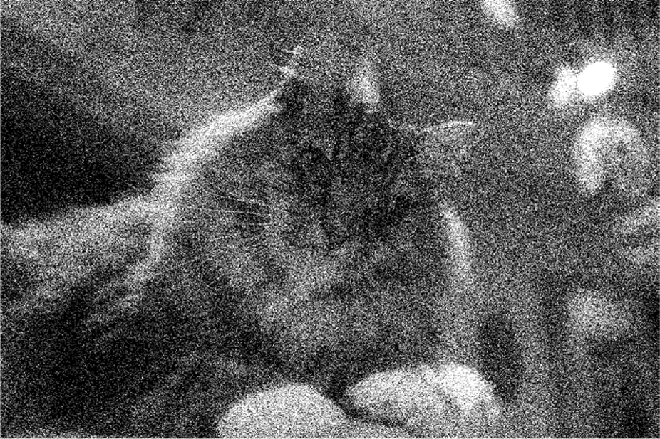
Figure 11-52: Tony dithered using random numbers
This eliminates the patterning artifacts but is pretty fuzzy, which is not unusual for cats. It’s not as good as the ordered dither.
The fundamental problem behind all these approaches is that we can only do so much making decisions on a pixel-by-pixel basis. Think about the difference between the original pixel values and the processed ones. There’s a certain amount of error for any pixel that wasn’t black or white in the original. Instead of discarding this error as we’ve done so far, let’s try spreading it around to other pixels in the neighborhood.
Let’s start with something really simple. We’ll take the error for the current pixel and apply it to the next horizontal pixel. The pseudocode is in Listing 11-24, and the result is shown in Figure 11-53.
for (y = 0; y < height; y++)
for (error = x = 0; x < width; x++)
if (value_of_pixel_at(x, y) + error > 127)
draw_white_pixel_at(x, y);
error = -(value_of_pixel_at(x, y) + error);
else
draw_black_pixel_at(x, y);
error = value_of_pixel_at(x, y) + error;
Listing 11-24: One-dimensional error propagation pseudocode
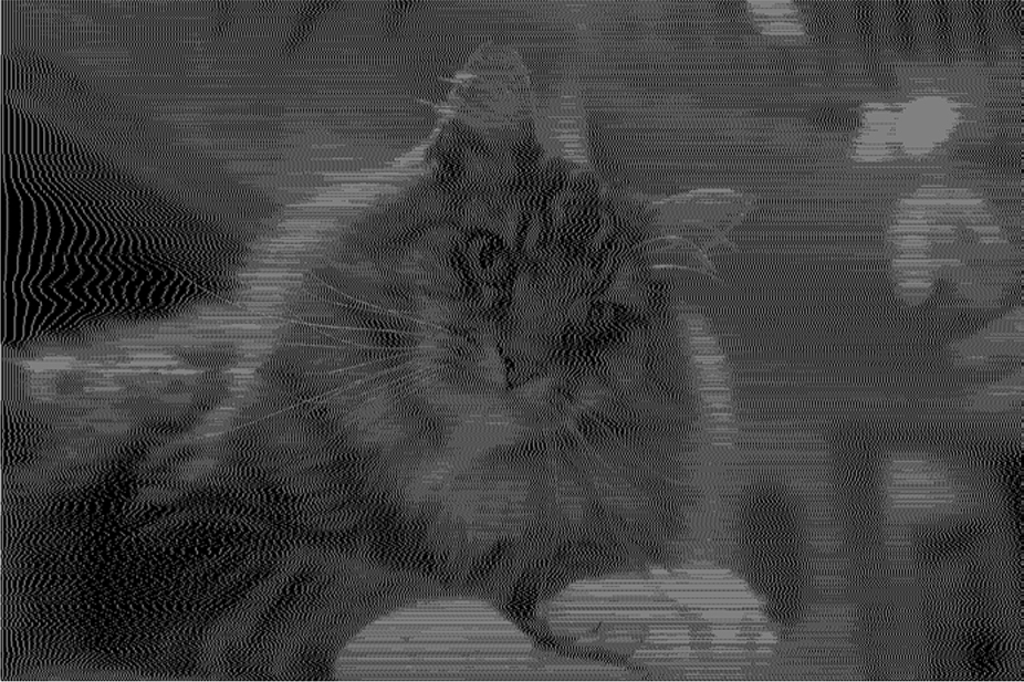
Figure 11-53: Tony dithered using one-dimensional error propagation
Not great, but not horrible—easily beats thresholding and random numbers and is somewhat comparable to the 2×2 matrix; they each have different types of artifacts. If you think about it, you’ll realize that error propagation is the same decision variable trick that we used earlier for drawing lines and curves.
American computer scientists Robert Floyd (1936–2001) and Louis Steinberg came up with an approach in the mid-1970s that you can think of as a cross between this error propagation and a Bayer matrix. The idea is to spread the error from a pixel to some surrounding pixels using a set of weights, as shown in Figure 11-54.
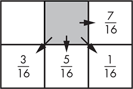
Figure 11-54: Floyd-Steinberg error distribution weights
Listing 11-25 shows the Floyd-Steinberg pseudocode. Note that we have to keep two rows’ worth of error values. We make each of those rows 2 longer than needed and offset the index by 1 so that we don’t have to worry about running off the end when handling the first or last columns.
for (y = 0; y < height; y++)
errors_a = errors_b;
errors_b = 0;
this_error = 0;
for (x = 0; x < width; x++)
if (value_of_pixel_at(x, y) > bayer_matrix[y % matrix_size][x % matrix_size])
draw_white_pixel_at(x, y);
this_error = -(value_of_pixel_at(x, y) + this_error + errors_a[x + 1]);
else
draw_black_pixel_at(x, y);
this_error = value_of_pixel_at(x, y) + this_error + errors_a[x + 1];
this_error = this_error * 7 / 16;
errors_b[x] += this_error * 3 / 16;
errors_b[x + 1] += this_error * 5 / 16;
errors_b[x + 2] += this_error * 1 / 16;
Listing 11-25: Floyd-Steinberg error propagation code
This is a lot more work, but the results, as shown in Figure 11-55, look pretty good. (Note that this is unrelated to the Pink Floyd–Steinberg algorithm that was used to make album covers in the 1970s.)
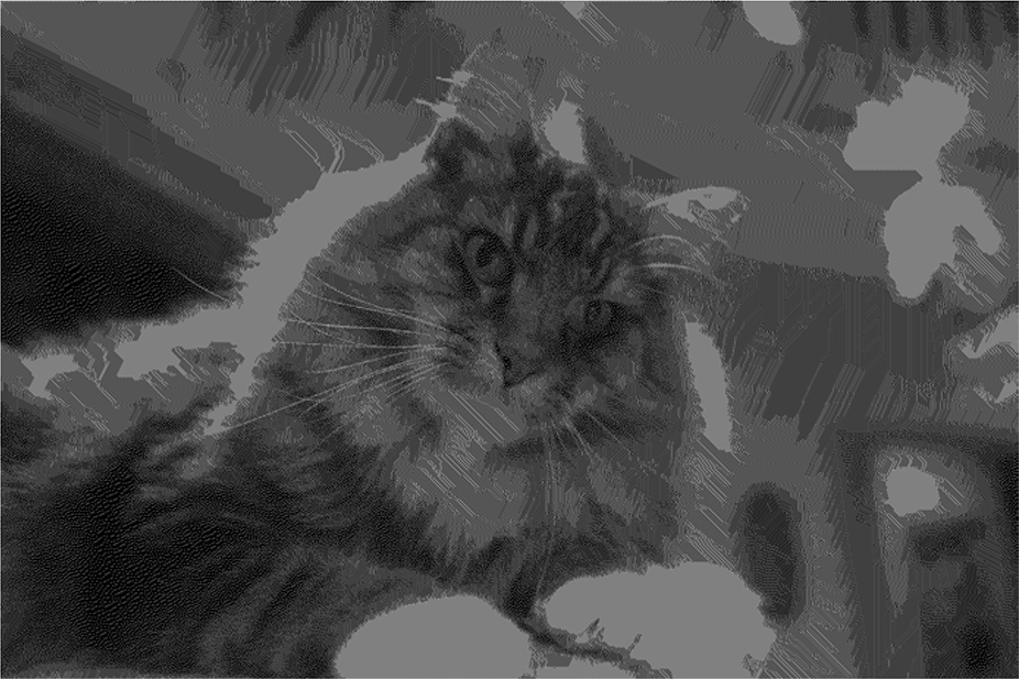
Figure 11-55: Tony dithered using the Floyd-Steinberg algorithm
Post–Floyd-Steinberg, numerous other distribution schemes have been proposed, most of which do more work and distribute the error among more neighboring pixels.
Let’s try one more approach, this one published by Dutch software engineer Thiadmer Riemersma in 1998. His algorithm does several interesting things. First, it goes back to the approach of affecting only one adjacent pixel. But it keeps track of 16 pixels’ worth of error. It calculates a weighted average so that the most recently visited pixel has more effect than the least recently visited one. Figure 11-56 shows the weighting curve.
Figure 11-56: Riemersma pixel weights
The Riemersma algorithm doesn’t use the typical adjacent pixels grid that we’ve seen before (see Listing 11-26). Instead, it follows the path of a Hilbert curve, which we saw in Figure 11-38.
for (each pixel along the Hilbert curve)
error = weighted average of last 16 pixels
if (value_of_pixel_at(x, y) + error > 127)
draw_white_pixel_at(x, y);
else
draw_black_pixel_at(x, y);
remove the oldest weighted error value
add the error value from the current pixel
Listing 11-26: Riemersma error propagation pseudocode
The result is shown in Figure 11-57. Still not purr-fect, but at this point we’ve seen enough cats. Try the example code on a gradient such as the one in Figure 11-12. You’ve learned that there are many different ways to deal with approximation required by real-life circumstances.
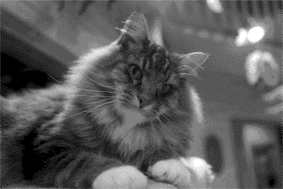
Figure 11-57: Tony dithered using the Riemersma algorithm
Summary
In this chapter, we’ve examined a number of tricks you can use to increase performance and efficiency by avoiding or minimizing computation. As Jim Blinn, one of the giants in the field of computer graphics, said, “A technique is just a trick that you use more than once.” And just as you saw with hardware building blocks, these tricks can be combined to solve complex problems.