CHAPTER 2

FUNDAMENTALS OF PATTERN ANALYSIS: A BRIEF OVERVIEW

BASABI CHAKRABORTY

2.1 INTRODUCTION

With the rapid proliferation of the use of computers, a vast amount of data are generated in every area of engineering and scientific disciplines (biology, psychology, medicine, marketing, finance, etc.). This vast amount of data with potentially useful information needs to be analyzed automatically for extraction of hidden knowledge. Pattern analysis is the process of automatically detecting patterns characterizing the inherent information in data. A pattern is defined in [1] as opposite of chaos; It is an entity, vaguely defined, that could be given a name. The objective of pattern analysis is to identify the patterns into some known categories–classes or to group the patterns in different categories that are then assigned some tags–class names. The former is known as supervised pattern classification and the later is known as unsupervised pattern classification or clustering.

The area of pattern analysis or pattern classification is not a new one, the research began during the 1950s and varieties of techniques [2–4] have been developed over the years. The survey papers of Unger [5], Wee [6], and Nagy [7] represent an account of the earlier works done in this area. Classical data analysis techniques for pattern discovery are based mainly on statistics and mathematics [8–10]. An excellent overview of statistical pattern recognition techniques is available in [11]. Though statistical techniques are well developed, they seem to be no longer adequate for analyzing an increasingly huge collection of complex data in a variety of domains (e.g., the worldwide web, bioinformatics, healthcare, or scientific research). Recently, new intelligent data analysis technologies are emerging based on soft computing tools (e.g., artificial neural network, fuzzy logic, and rough sets), evolutionary techniques, and genetic algorithm to deal with imprecision and uncertainty in complex data [12–18].

This chapter represents an introduction to the fundamental concept behind pattern recognition techniques and a brief overview of the methodologies developed to date. Section 2.2 introduces the basic concepts behind pattern analysis and different approaches for designing a pattern recognition system. The following sections deal with the key processes of pattern analysis and a brief overview of the presently available techniques. Emphasis has been given to statistical techniques, the pioneering contributor in the field of pattern analysis. Section 2.7 concludes with a discussion of future issues.

2.2 PATTERN ANALYSIS: BASIC CONCEPTS AND APPROACHES

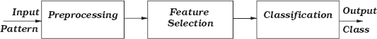
The basic steps of an automatic pattern analysis system are shown in Figure 2.1. The numerical representation of the pattern constitutes the measurement space. The lower dimensional representation of the measurement space constitutes the feature space and the categorization of the pattern represents the decision space. The role of the preprocessing step is to separate the pattern of interest from noisy background, and other necessary operations for suitable processing in the next step. Feature selection or feature extraction is to select–extract discriminatory features for representing the input pattern in a compact way for correct classification in the next stage, while discarding redundant information. The final step classifies input patterns to one of the possible classes or groups the patterns into some categories according to similarities among them. The accuracy of an automatic pattern recognition system depends jointly on the performance of the feature selector and the classifier. The degradation at any stage affect the efficiency of the other stage resulting in an overall inefficient system.

The different approaches for pattern analysis developed so far can be categorized into four areas: which are (1) template matching, (2) statistical approach, (3) syntactic approach, and (4) the soft computing approach. Some attempts also have been made to design hybrid systems with combinations of different approaches. A brief description of the different approaches are presented below.

2.2.1 Template Matching

The simplest and earliest approach to pattern recognition is based on template matching. The input pattern to be classified is matched against the reference patterns called the templates of the available classes. The reference patterns are learned from the training samples and matching is done by using a similarity measure, mostly correlation measures. This approach is used mostly in the application of text or string matching. Dynamic programming based techniques [19] are the popular example of template matching [20,21]. The rigid template matching approach is not suitable for pattern analysis problems where the intraclass variation is large.

2.2.2 Syntactic Approach

For hierarchical patterns, where a pattern is composed of simple subpatterns that are themselves composed of simpler subpatterns, the syntactic approach is efficient for analysis [22]. In syntactic approach, a formal analogy is drawn between the structure of patterns with a syntax of a language. The simplest patterns are called primitives and the complex patterns are formed by interconnecting primitives according to some defined rules (e.g., rules of grammar in a language). Thus the patterns are described by primitives and grammatical rules. The grammatical rules for each class are assessed from the training samples. This approach is useful for the non-numeric patterns having definite structure.

2.2.3 Statistical Approach

Among all the approaches, statistical pattern recognition has gained the widest acceptance. In classical statistical pattern analysis [9], a pattern is represented by a set of n features, or attributes, viewed as an n-dimensional feature vector (the points in n-dimensional measurement space Rn) are represented as x = (x1, x2, … xn)T. Feature selection process transforms the pattern vector from n-dimensional measurement space to a d-dimensional feature space, where d ≤ n. Recognition or classification process classifies or groups the patterns into one of the m possible classes. The statistical techniques for pattern analysis are represented in brief in the following sections.

2.2.4 Soft Computing Approach

Different computing tools (e.g., artificial neural network, fuzzy logic, rough set, genetic algorithm and evolutionary computation, and their integration to deal with impreciseness and uncertainty in real-world pattern analysis problems are collectively known as soft computing tools. Recently, these tools are increasingly used for pattern analysis. A brief presentation of soft computing approaches is presented in the later section.

2.3 FEATURE SELECTION

Feature selection or extraction is one of the major steps in an automatic pattern analysis system. The main objective of feature selection is to retain the optimum discriminatory information and to reduce the dimensionality of the measurement space from n to d (d ≤ n) to facilitate classification or recognition processes. The pioneering works on feature selection deals mostly with statistical tools and the major techniques developed so far can be broadly classified into two categories:

2.3.1 Feature Selection in Measurement Space

Feature selection in measurement space or feature subset selection selects a subset of d features from a set of n features on the basis of their quality in discriminating classes. Feature subset selection techniques are based on the design of a criterion function and the selection of a search strategy. The criterion function evaluates the goodness of a feature and ranks them. The best two features may not be the best feature subset of two features when used in combination [23]. So, we need a search strategy to decide the best possible feature subset among a number of candidates.

2.3.1.1 Feature Evaluation Measures. There are several approaches to evaluate the goodness of a feature subset. Some of the popular measures are listed here. The details can be found in [8].

2.3.1.1.1 Measures Based On Error Probability. Pattern classification is a decision-making process in which an input pattern in an n-dimensional feature space, defined by f = [f1,f2,…, fn], is assigned to one of a number of possible classes wi, where i = 1,2, …, m, depending on the value of the feature vector. Let the a priori probability of occurrence of a class wi be P(wi), and let the multivariate class-conditional probability density function of class wi be p(f| wi). The mixture density function p(f) is given by

According to Bayes’ rule [2], the a posteriori probability for the ith class is

and according to Bayes’ decision procedure, an unknown input pattern is assigned to class wi if

The objective of any pattern recognition process is to classify unknown patterns with the lowest possible probability of misrecognition. The objective for designing the feature selection criterion should be such that the error probability pe is minimized. In an n-dimensional feature space f, the error probability pe is given by

Although the error probability is, from the theoretical viewpoint, the ideal measure for designing the feature selection criterion, it is not easy to evaluate from the practical computational point of view. Therefore a number of alternative criteria for feature evaluation have been suggested so far. Most of the indirect measures have been developed based on the concept of distance, separability, overlap, or dependence between the probability distributions characterizing the pattern classes.

2.3.1.1.2 Measures Based On Class Separability. The discriminatory power of any feature is associated with the concept of class separability. The interclass distance between two classes w1 and w2 is the simplest concept of class separability and can easily be used to assess the discriminatory potential of a feature in pattern representation. This measure is not defined explicitly by class-conditional probability density functions. Its estimate based on elements of the training set can be computed directly without prior determination of the probabilistic structure of the classes. Thus, separability measures based on this concept cannot serve as true indicators of the mutual overlap of the classes,though it is very simple to evaluate. The measures derived from the concept of class separability that are normally used in practice are divided into the following three groups:

Now, pe is maximum when the integrand is zero (i.e., the density functions are completely overlapping, and pe is zero when the functions do not overlap. The integral in Eq. (2.5) can be considered to quantify the “probabilistic distance” between the two density functions. The greater the distance, the smaller the error, and vice versa. Any other measure of “distance” between the two density functions, such as

satisfying J ≥ 0 can be used as a feature evaluation criterion. Here J = 0 when p(f|wi), i=1,2 are overlapping and J is maximum when p(f|wi), i=1,2 are nonoverlapping.

The most commonly used probabilistic distance measure are given below:

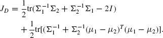
Bhattacharya Distance. Bhattacharya distance function is defined as follows:

For multivariate Gaussian distributions where

μi and Σi represent a mean vector and covariance matrix for the probability distribution of the feature for the ith class, respectively.

The Jeffreys–Matsusita Distance Measure. The Jeffreys–Matushita distance measure JM is defined to be

Note that the Jeffreys–Matushita and Bhattacharya distance are two different variations of the same measure and the relationship between them is given by

Divergence Function. The divergence function was first introduced by Jeffreys and is defined by

Later it was developed by Toussaint and for the multivariate Gaussian distribution, the divergence function becomes

Mahalanobis Distance. For two multivariate distributions with common dispersion matrix, the Mahalanobis distance is given as

This distance function is very easy to compute though it is difficult to make theoretical assessment of the accuracy in a distribution-free case.

Kolmogorov Variational Distance. The Kolmogorov variational distance is defined to be

From this measure, the probability of error pe can be determined directly by the equation

but the computational difficulty associated with this measure is the same as that for pe.

There are several other measures, developed from time to time, by the researchers. A complete discussion on their relative merits and demerits in evaluating feature quality is available in [24].

Bhattacharyya

Matushita Distance

Patric–Fisher Distance

where α is a real, positive parameter. For α = 1, the measure becomes

which is the separability measure based on the well-known Shannon entropy. The optimal feature set can be obtained by minimizing the above criterion.

Entropy can also be used without the knowledge of densities as in decision tree algorithm [26], where the information gain with the inclusion–deletion of features are independently computed.

2.3.1.2 Search Strategies. The selection of an optimal feature subset of d features from a set of n features on the basis of a feature evaluation measure becomes a difficult search problem when n is large.

The two main approaches by which suboptimal solutions to the problem can be achieved are forward and backward selection [8]. A lot of search algorithms of different variants (sequential search, random search [27] of the two main approaches and their combinations have been developed for feature subset selection process. One of the popular techniques is branch and bound developed by Narendra and Fukunaga [28] and its variants [29]. A good survey of search strategies for feature subset selection can be found in [2,30,31].

2.3.1.3 Feature Selection Algorithms. The existing approaches of a feature subset selection can also be viewed as broadly classified into two categories: filter and wrapper approaches. Filter approaches [32, 33] are based on a criterion function that is classifier independent, while wrapper approaches [34] use the classifier accuracy as the criterion function and depends on the learning algorithm of the specific classifier. The two approaches have basic merits and demerits. While classifier dependant methods produce good results, especially when the classifier is designed to solve the particular problem, it is not computationally attractive when the number of input features are large. The computational burden is more heavy when a nonlinear classifier with complex learning algorithms are used.

2.3.2 Feature Selection in Transformed Space

The feature selection in transformed space is commonly known as a feature extraction method that uses all the information contained in a pattern vector and maps the higher dimensional pattern vector to a lower dimensional one. The objective of transformation, linear or nonlinear, is also to make original features uncorrelated to remove redundancy. The mathematical mapping techniques are computationally simpler than the probabilistic criteria and produce satisfactory results in practical situations, but unlike the probabilistic criteria they do not have any relationship with the error probability.

Linear transformation (e.g., principal component analysis, PCA), factor analysis, linear discriminant analysis, independent component analysis, and projection pursuit [2] are widely used in pattern analysis. The PCA or K-L transform is the most popular one in which d largest eigenvectors of the covariance matrix of the n-dimensional patterns are used for representation of the pattern. A lot of transforms [e.g., Fourier transform (FT) and its variants DFT, FFT, Harr transform, direct cosine transform (DCT)] are popular in spatial pattern analysis. Kernel PCA [35], multidimemsional scaling (MDS) [36], and artificial neural network-based [37, 38] methods are examples of nonlinear transformation. A comparative study of feature selection algorithms can be found in [39].

2.3.3 Soft Computing Approaches for Feature Selection

Recently, many feature selection algorithms based on soft computing approaches [40, 41], mainly artificial neural network, fuzzy set, genetic algorithm, and evolutionary computation and their hybrids [17], have been developed for solving real-world problems, where statistical methods are difficult to apply. Artificial neural network-based approaches are found in [38,42–44]. In [45], a fractal neural network architecture is proposed and is used as a feature selector. The self-organization map (SOM) [46] or autoassociative networks [47] can be used as a nonlinear feature extractor. A comparative review of neural network feature extractor is found in [48].

In [49], fuzzy set theoretic measure based on the index of fuzziness and fuzzy entropy is developed for feature evaluation and ranking. Some hybrid neuro-fuzzy approaches are reported in [50–52]. Feature selection algorithm based on rough set theory and hybrid approaches are reported in [53–56]. Genetic algorithm (GA, widely used in optimization problems, is also a good candidate for feature subset selection and a number of GA based and hybrid algorithms are developed in this different application area. Some of them are reported in [57–63]. Other evolutionary computational techniques, like particle swarm optimization (PSO) and their hybrids with other soft computing tools, recently have been used for feature selection problems [64–69].

2.4 PATTERN CLASSIFICATION

The final and ultimate goal of pattern analysis is to classify the input patterns to known classes or to group them in different categories depending on their similarity. When the class information is available, the pattern analysis system learns from the training samples. The unknown input pattern, when presented to the learned system, is identified as a member of one of the known classes. This paradigm, known as supervised classification, is represented in this section.

2.4.1 Statistical Classifier

In supervised classification, a set of patterns having known class information are used as training samples by which the classifier learns the decision rule with some suitable algorithm. The learned classifier then categorizes the unknown input pattern to one of the classes with the help of the learned decision rule. Lots of learning algorithms using statistical concepts have been developed and are based on them and a variety of classifiers now have been designed. Statistical classification methods can be broadly classified into three groups [11]. The simplest and most intuitive approach is based on similarities measured by some distance function [70]. Here the proximity of a pattern to a class serves as the measure for its classification. Minimum distance classifier, nearest-neighbor algorithm [8], and its variants are the popular techniques in this category. The most advanced techniques for computing prototypes are vector and learning vector quantization [46].

2.4.1.1 k-NN Classifier. The k nearest-neighbor (k-NN) classifier is one of the earliest, simpliest, and most popular classifier. The algorithm known as the k-NN decision rule, can be stated as follows: Given an unknown pattern vector x and a distance measure,

For k = 1 the algorithm is simply known as the nearest-neighbor rule. Various distance measures can be used including the simplest Euclidean and Mahalanobis. For large values of n, this simple classifier can show quite a good performance.

2.4.1.2 Bayes Classifier and Discriminant Analysis. The main approachs of statistical methods are the probabilistic approach and the famous Bayes classfier [2,8], based on Bayes decision rule, which has been developed for a known class of conditional probability densities p(x|wi). A number of well-known decision rules, including Bayes decision rule, the maximum likelihood rule, and the Neyman–Pearson rule are available to generate the decision boundary. First, according to the Bayes decision rule, an input pattern x is assigned to class wi for minimum error or minimum risk of classification if,

P(wi| x) is the a posteriori probability for class wi.

Using Bayes rule of probability, the above rule can be effectively expressed using class conditional probability densities.

In practice, the estimates of densities are used in place of true densities. The density estimates are either parametric, where the distribution of the feature vectors are known, nonparametric, or distribution free methods. Commonly used parametric models are Gaussian distributions given as

where i = 1,2,…, m, μi = E[x] denotes the mean value of class wi, Σi denotes the n× n covariance matrix defined as

A variety of density estimators for the nonparametric approach from simple histogram estimators, followed by window estimators and kernel estimators, are available in the literature [2,8].

The equation for the decision surface of the two regions containing the ith and jth class is given by

Now gi(x), a monotonically increasing function representing f(P(wi| x)), is known as discriminant function. Thus the decision rule can be stated as follows in Eqs. (2.25) and (2.26).

Classify the pattern x in class wi if

and the equation of decision surface separating two regions becomes

Linear discriminant analysis is another category of approaches to construct decision boundaries or decision surface by optimizing certain error criterion. When the estimate of densities are difficult, it is preferable to compute decision surfaces directly by alternative costs. Such approaches gives rise to linear discriminant analysis and design of many linear classifiers. Linear discriminant analysis (LDA) approximates boundaries between classes by placing hyperplanes optimally assuming the classes to be linearly separable. The limitations of linear classifiers for nonlinearly separable classes prompted the development of nonlinear classifiers. A comparative study of various statistical classifiers can be found in [71].

2.4.1.3 Decision Tree Classifier. Decision tree classifiers [26] are a special type of nonlinear classifier. They are multistage decision systems that iteratively select an individual feature to partition the feature space generating a tree structure. The leaf nodes represent the final classification. Selection of a feature at each node is done according to some criterion function (e.g., information content). Though these classifiers are suboptimal, they are popular due to the fast classification ability and the rule generation with individual features making the classification process transparent to users.

2.5 UNSUPERVISED CLASSIFICATION OR CLUSTERING

When class information is not available, the input patterns are grouped into some classes or clusters according to their similarity. This paradigm of classification is known as unsupervised classification or cluster analysis in the context of pattern analysis. Clustering is one of the primitive mental activities of humans to deal with huge amounts of information they receive every day. Remembering every piece of information is difficult and humans tend to categorize entities into clusters. Cluster analysis is applied to different areas and has a long history of research. The early works can be found in [72,73]. More recent algorithms can be found in [74]. Like the case of supervised classification, a pattern here is also represented in terms of n-dimensional vectors. The basic steps of the clustering task are as follows:

2.5.1 Definition of Clustering and Proximity Measure

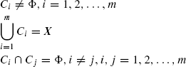
Let X be a set of N pattern vectors, that is, X = (x1,x2, …, xN). An m clustering of X partitions the pattern space into m sets C1, C2, …, Cm, such that

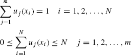
As there is an overlapping of categories for real-world data, crisp clustering defined above cannot handle them. Fuzzy clustering [81] of X into m clusters in which all the patterns can belong to several clusters with a varying degree of membership functions uj can be defined below as:

and

A proximity measure can be defined in terms of either a dissimilarity measure (DM) or a similarity measure (SM). A similarity measure is intuitively opposite to a DM. Now, a DM d on X is a function

where R is the set of real numbers, such that

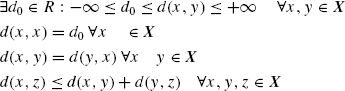
The simplest dissimilarity metric is the Euclidean distance and is widely used as DM in clustering applications. There are also other DMs (Manhattan distance, point symmetric metric etc.).

The most common SM is an inner product

The Hamming distance, Tanimoto measure, and so on, are other examples of SMs.

2.5.2 Clustering Algorithms

Clustering algorithms available in the literature can be divided into the following major categories:

2.6 NEURAL NETWORK CLASSIFIER

Artificial neural networks, the most widely used soft computing paradigm, have recently emerged as an important tool for data analysis and pattern classification. Their effectiveness in both supervised and unsupervised classification has been tested empirically and many applications in a variety of real-world classification tasks have been developed [12, 14, 86]. A survey of neural network classifiers can also be found in [87]. Links between neural and other conventional classifiers are discussed in [47, 88]. Performance comparisons of neural network classifiers and conventional statistical classifiers also have been studied in a number of works. Some of them are reported in [89, 90]. Riplay [91] compared neural networks with various classifiers (e.g., classification tree, projection pursuit, linear vector quantization, and nearest-neighbor methods).

Although many types of neural networks are used in classification problem, the most widely studied neural network for classification purposes is the feedforward multilayer perceptrons (MLP). One of the pioneer works on the use of MLP for pattern classification is studied in [92]. In [93], fractal neural network architecture is proposed and its performance as a classifier has been studied in comparison to MLP. It was found that it is well suited for classification of fractal patterns. Other architectures (e.g., radial basis function, RBF, networks [46], support vector machines (SVM) [96] and are also developed for supervised classification. Self-organizing map (SOM) or a Kohonen Network [46] is applied to unsupervised classification.

Although significant progress has been made in neural network-based classification for real-world problems, there are still some unresolved issues. Though neural networks do not require explicit knowledge of underlying distribution of patterns like statistical classifiers, their classification process in most of the cases is not transparent. This blackbox characteristics of neural architecture poses problem for generating explicit decision rules. To avoid this, some hybrid approaches combining neural network with a rough set or fuzzy logic have also been studied recently [17].

2.7 CONCLUSION

This chapter presents a brief overview of the fundamental techniques of pattern analysis. Pattern analysis is an important process for knowledge extraction from raw data generated everyday in different areas of human interest. With the progress of computing technologies, large amounts of data in recently discovered areas (e.g., molecular biology or genomic research), is now becoming available daily. This huge amount of data needs to be processed in order to extracting hidden information. Though the techniques of pattern analysis have grown for a long time and well-known tools are available, the demand for development of newer and more powerful techniques is also increasing due to the generation of newer and newer varieties of data.

Thus, the importance of research for improving pattern analysis techniques is ever increasing. For the development of new techniques, one should be fully aware of the basic concepts of fundamental pattern analysis techniques. This chapter attempts to represent the basic concepts and approaches behind pattern analysis techniques. A brief overview of the important and most popular statistical tools are explained. Recent approaches based on the soft computing paradigm are also introduced with a brief representation of the promising neural network classifiers as a new direction toward dealing with imprecise and uncertain patterns generated in newer fields.

REFERENCES

1. S. Watanabe (1985), Pattern Recognition: Human and Mechanical, New York, Jonh Wiley & Sons, Inc., NY.

2. R. O. Duda and P. E. Hart (1973), Pattern Classification and Scene Analysis, Wiley, NY.

3. R.O. Duda, P. E. Hart, and D. G. Stork (2001), Pattern Classification, 2nd ed., John Wiley & Sons, Inc., NY.

4. S. Theodoridis and K. Koutroumbas (1999), Pattern Recognition, Academic Press, San Diego.

5. S. H. Unger (1959), Pattern detection and recognition, Proc. IR, 47: 1737–1752.

6. W. G. Wee (1968), A survey of pattern recognition, IEEE Proc. Seventh Symp. Adaptive Proc., 2.e.1–2.e.1.

7. G. Nagy (1968), State of the art in pattern recognition, Proc. IEEE, 56: 836–862.

8. P. A. Devijver and J. Kittler (1982), Pattern Recognition: A Statistical Approach, Prentice-Hall, London.

9. K. Fukunaga (1990), Introduction to Statistical Pattern Recognition, Academic Press, NY.

10. L. Devroye, L. Gyorfi and G. Lugosi (1996), A Probabilistic Theory of Pattern Recognition, Springer, NY.

11. A. K. Jain, R. P. W. Duin, and J. Mao (2000), Statistical Pattern Recognition : A Review, IEEE Trans. PAMI, 22(1): 4–37.

12. C. M. Bishop (1995), Neural Networks for Pattern Recognition, Oxford University Press, NY.

13. C. M. Bishop (2006), Pattern Recognition and Machine Learning, Springer Science+ Business Media, NY.

14. B. D. Ripley (1996), Pattern Recognition and Neural Networks, Cambridge University Press, NY.

15. Y. H. Pao (1989), Adaptive Pattern Recognition and Neural Networks, Addison-Wesley, NY.

16. S. K. Pal and D. Dutta Majumder (1986), Fuzzy Mathematical Approach to Pattern Recognition, Wiley (Halsted Press), NY.

17. S. K. Pal and S. Mitra (1999), Neuro-Fuzzy Pattern Recognition: Methods in Soft Computing, John Wiley & Sons, Inc., NY.

18. S. K. Pal and A. Pal (eds.) (2001), Pattern Recognition: From Classical to Modern Approaches, World Scientific, NY.

19. R. E. Bellman (1957), Dynamic Programming, Princeton University Press, Princeton, NY.

20. H. Sakoe and S. Chiba (1978), ‘Dynamic programming algorithm optimization for spoken word recognition’, IEEE Trans. Acous, Speech Signal Proc., 26:(2): 43–49.

21. H. Silverman and D. P. Morgan (1990), The application of the dynamic programming to connected speech recognition, IEEE Signal Proc. Mag., Vol. 7(3): 7–25.

22. K. S. Fu (1982), Syntactic Pattern Recognition and Applications, Prentice-Hall, NJ.

23. T. M. Cover (1974), The Best Two Independent Measurements are not the Two Best, IEEE Trans. SMC, 4: 116–117.

24. C. B. Chittineni (1980), Efficient feature subset selection with probabilistic distance criteria, Infor Sci., 22: 19–35.

25. M. Ben-Bassat (1982), Use of Distance Measures, Information Measures and Error bounds in Feature Evaluation, Handbook of Statistics, 2: 773–791, North-Holland.

26. J. R. Quinlan (1993), Programs for Machine Learning, Morgan Kaufman, CA.

27. H. Liu and H. Motoda (1998), Feature Selection for Knowledge Discovery and Data Mining, Kluwer Academic Publishers, London.

28. P. Narendra and K. Fukunaga (1977), A Branch and Bound Algorithm for Feature Subset Selection, IEE Trans. Computer, C-26(9): 917–922.

29. I. Foroutan and and J. Sklansky (1987), Feature selection for automatic classification of non-gaussian data, IEEE Trans. SMC, 17(2): 187–198.

30. W. Siedlecki and J. Sklansky (1988), On Automatic Feature Selection, Inter. J. Pattern Recogn. Art. Intell., 2: 197–220.

31. M. Dash and H. Liu (1997), Feature Selection for Classification, Intelligent Data Analysis, 1: 131–156.

32. H. Almuallim and T. G. Dietterich (1994), Learning boolean concepts in the presence of many irrelevant features, Arti. Intell., 69: 279–305.

33. K. Kira and L. A. Rendell (1992), The feature selection problem: Traditional methods and a new algorithm, Proceedings of Ninth National Conference on Artificial Intelligence, MIT Press, Cambridge, MH, pp. 129–134.

34. G. H. John, R. Kohavi, and K. Pfleeger (1994), Irrelevant feature and the subset selection problem, Machine Learning: Proceedings of the Eleventh International Conference, pp. 121–129.

35. B. Scholkopf, A. Smola, and K. R. Muller (1998), Nonlinear Component analysis as a Kernel Eigenvalue Problem, Neural Comput., 10(5): 1299–1319.

36. I. Borg and P. Groenen (1977), Mordern Multidimensional Scaling, Springer-Verlag, Berlin.

37. S. Haykin (1999), Neural Networks, A Comprehensive Foundation, Prentice-Hall, NJ.

38. R. Setiono and H. Liu (1997), Neural Network Feature Selector, IEEE Trans. NN, 8(3): 654–662.

39. M. Kudo and J. Sklansky (2000), Comparison of Algorithms that Select Features for Pattern Recognition, Pattern Recog., 33(1): 25–41.

40. N. R. Pal (1999), Soft computing for feature analysis. Fuzzy Sets Systems, 103: 201–221.

41. B. Chakraborty (2002), Integration of Soft Computing Approaches for Feature Selection in Pattern Recognition Problems, J. IETE, 48(5): 403–413.

42. D. W. Ruck, S. K. Rogers, and M. Kabrisky (1990), Feature selection using a multilayer perceptron, Neural Network Comput., 20: 40–48.

43. A. Verikas and M. Bacauskiene (2002), Feature selection with neural networks, Pattern Recog. Lett., 23(11): 1323–1335.

44. N. Kwak and C.-H. Choi (2002), Input feature selection for classification problems, IEEE Trans. Neural Networks, 13(1): 143–159.

45. B. Chakraborty and Y. Sawada (1999), Fractal Neural Network Feature Selector for Automatic Pattern Recognition System, IEICE Trans. Fund. Elect. Commun. Comput. Sci., E82-A(9): 1845–1850.

46. T. Kohonen (2001), Self Organizing Maps, Springer, NY.

47. E. Oja (1997), The Nonlinear PCA Learning Rule in Independent Component Analysis, Neurocomputing, 17(1): 25–45.

48. B. Lerner, H. Guterman, M. Aladjem, and I. Dinstein (1999), A comparative Study of Neural Network based Feature Extraction, Pattern Recogn. Lett., 20(1): 7–14.

49. S. K. Pal and Basabi Chakraborty (1986), Fuzzy set Theoretic Measure for Automatic Feature Selection, IEEE Trans. Sys, Man Cybernetics, SMC-16(5): 754–760.

50. S. K. Pal, R. K. De, and J. Basak (2000), Unsupervised feature evaluation: a neuro-fuzzy approach, IEEE Trans. Neural Networks, 11(2): 366–376.

51. B. Chakraborty and G. Chakraborty (2001), A Neuro Fuzzy Algorithm for Feature Subset Selection, IEICE Trans. Fund. Elect. Commun. Comput. Sci., E84-A(9): 2182–2188.

52. B. Chakraborty (2000), Feature Selection by Artificial Neural Network for Pattern Classification, Pattern Recognition in Soft Computing Paradigm, Vol. 2 of FLSI Soft Computing Series, World Scientific, NY. pp. 95–109.

53. M. Quafafou and M. Boussouf (2000), Generalized rough set based feature selection, Intelligent Data Anal., 4(1) 3–17.

54. M. Zhang and J. T. Yao, (2004), A rough set based approach to feature selection, Proc. NAFIPS, 1: 434–439.

55. R. Jensen and Q. Shen (2007), Rough set based feature selection: A review, Rough Computing: Theories, Technologies and Applications, IGI Global, pp. 70–107.

56. R. B. Bhatt and M. Gopal (2005), On fuzzy-rough set approach to feature selection, Pattern Recog. Lett., 26(7): 965–975.

57. W. Siedlecki and J. Sklansky (1989), A note on genetic algorithms for large-scale feature selection, Pattern Recog. Lett., 10(5): 335–347.

58. M. L. Raymer, W. F. Punch, E. D. Goodman, L. A. Kuhn, and A. K. Jain (2000), Dimensionality reduction using genetic algorithms, IEEE Trans. EC, 4(2): 164–171.

59. J. S. Lee, I. S. Oh, and B. R. Moon (2004), Hybrid Genetic Algorithm for Feature Selection, IEEE Trans. PAMI, 26(11): 1424–1437.

60. F. Hussein, N. Kharma, and R. Ward (2001), Genetic algorithms for feature selection and weighting, a review and study, Proccedings of Sixth International Conference on Document Analysis and Recognition, pp. 1240–1244.

61. B. Chakraborty (2002), Genetic Algorithm with Fuzzy Operators for Feature Subset Selection, IEICE Trans. Fund. Electr. Commun. Comput. Sci., E85-A(9): 2089–2092.

62. J. Huang, Y. Cai, and X. Xu (2007), A hybrid genetic algorithm for feature selection wrapper based on mutual information, Pattern Recog. Lett., 28(13): 1825–1844.

63. J. Lu, T. Zhang, and Y. Zhang (2008), Feature selection based-on genetic algorithm for image annotation, Knowledge Based Systems, 21(8): 887–891.

64. Y. Liu et al. (2005), Feature Selection with Particle Swarms, LNCS, 3314: 425–430.

65. B. Chakraborty (2009), Binary Particle Swarm Optimization based Algorithm for Feature Subset Selection, Proceedings ICAPR09 (International Conference on Advances in Pattern Recognition 2009), pp. 145–148.

66. C. J. Tu, L. Y. Chuang, J. Y. Chang, and C. H. Yang (2006), Feature Selection using PSO-SVM, Proceedings of International Multiconference Engineers and Computer scientist, Association of Engineers, Hong Kong, pp. 138–143.

67. T. F. Lee, M. Y. Cho, and F. M. Fang (2007), Feature Selection of SVM and ANN using Particle Swarm Optimization for Power Transformers Incipient Fault Symptom Diagnosis, Intern. J. Comput. Intel. Res., 3(1): 50–65.

68. M. Shoorehdeli, M. Teshnehlab, and H. A. Moqhaddam (2006), Feature Subset Selection for face detection using genetic algorithms and particle swarm optimization, Proceedings of International Conference on Networking Sensing and Control, IEEE Internaltional Conference Networking, Sensing and Control, Ft. Louderdale, FL, pp. 686–690.

69. X. Wang, J. Yang, X. Teng, W. Xia, and R. Jensen (2007), Feature Selection based on Rough Sets and Particle Swarm Optimization, Pattern Recog. Lett., 28(4): 459–471.

70. J. T. Tou and R. C. Gonzalez (1974), Pattern Recognition Principles, Addison-Wesley, London.

71. S. Aeberhand, D. Coomas, and O. Devel (1994), Comparative analysis of statistical pattern recognition methods in high dimensional setting, Pattern Recog., 27(8): 1065–1077.

72. M. R. Anderberg (1973), Cluster Analysis for Applications, Academic Press, NY.

73. J. A. Hartigan (1975), Clustering Algorithms, Wiley, New York.

74. B. S. Everitt, S. Landau, and M. Leese (2001), Cluster Analysis, Arnold, London.

75. J. G. Dy and C. E. Brodly (2004), Feature Selection for Unsupervised Learning, J. Machine Learning Res., 5: 845–889.

76. J. Handl and J. Knowles (2006), Feature Subset Selection in Unsupervised Learning via Multiobjective Optimization, Inter. J. Comput. Intel. Res., 2(3): 217–238.

77. P. Mitra, C. A. Murthy, and S. K. Pal (2002), Unsupervised feature selection using feature similarity, IEEE Trans. PAMI, 24(3): 301–312.

78. M. Halkidi, Y. Batistatikis, and M. Vazirgiannis (2002), Cluster validity methods: part I, SIGMODD Rec., 31(2): 264–323.

79. M. Halkidi, Y. Batistatikis, and M. Vazirgiannis (2002), Cluster validity methods: part II, SIGMODD Rec., 31(3): 19–27.

80. X. L. Xie and G. Beni (2001), A validity measure for fuzzy clustering, IEEE Trans. PAMI, 23(6): 674–680.

81. J. C. Bezdek (1981), Pattern Recognition with Fuzzy Objective Function Algorithm, Plenum Press, New York.

82. J. C. Dunn (1973), A fuzzy relative of the ISODATA process and its use in detecting compact well separated clusters, J. Cybernetics, 3: 32–57.

83. U. Maulik and S. Bandyopadhyay (2000), Genetic Algorithm based Clustering Technique, Pattern Recog., 33(9): 1455–1465.

84. S. Saha and S. Bandyopadhyay (2007), A fuzzy genetic clustering technique using a new symmetry based distance for automatic evolution of clusters, Proceedings of ICCTA, IEEE Computer Society, pp. 309–314.

85. U. Maulik and S. Bandyopadhyay (2002), Performance evaluation of some clustering algorithms and validity indices, IEEE Trans. PAMI, 24(12): 1650–1654.

86. C. G. Loony (1997), Pattern Recognition using Neural Networks, Oxford University Press, NY.

87. G. P. Zhang (2000), Neural Networks for Classification: A Survey, IEEE Trans. SMC Part C, 30(4): 451–462.

88. B. Cheng and D. Titterington (1994), Neural networks: A review from statistical perspectives, Stat. Sci., 9(1): 2–54.

89. W. Y. Huang and R. P. Lippmann (1987), Comparisons between neural net and conventional classifiers, Proc. IEEE 1st. Int. Conf. NN, 485–493.

90. D. Michie et al. (1994), Machine Learning, Neural and Statistical Classification, Ellis Horwood, London.

91. A. Riplay (1994), Neural networks and related methods for classification, J. R. Statis. Soc B, 56(3): 409–456.

92. R. P. Lippmann (1989), Pattern classification using neural networks, IEEE Commun. Mag., 47–64.

93. B. Chakraborty, Y. Sawada, and G. Chakraborty (1997), Layered Fractal Neural Net: Computational Performance as a Classifier, Knowledge-Based Systems, 10(3): 177–182.

94. M. J. D. Powell (1985), Radial basis functions for multivariable interpolation: A review, IMA Conference on Algorithms for the Approximations of Functions and Data, IEEE Communication Sociaty, pp. 143–167.

95. W. A. Light (1992), Some aspects of radial basis function approximation, Approximations Theory, Spline Functions and Applications, Boston, Kluwer Academic Publishers, Boston, pp. 163–190.

96. V. N. Vapnik (1998), Statistical Learning Theory, Jonh Wiley & Sons, Inc., NY.