
CHAPTER 11
INTEGRATED DIFFERENTIAL FUZZY CLUSTERING FOR ANALYSIS OF MICROARRAY DATA
11.1 INTRODUCTION
In recent years, DNA microarrays has been developed as a popular technique for gathering a substantial amount of gene expression data that is necessary to examine complex regulatory behavior of a cell [1]. Microarray gene expression data, consisting of G genes and T time points, is typically organized in a two-dimensional (2D) matrix E = [eij] of size G × T. Each element eij gives the expression level of the it h gene at the jt h time point. Clustering [2–4], an important microarray analysis tool, is used to identify the sets of genes with similar expression profiles. Clustering methods partition the input space into K regions, depending on some similarity–dissimilarity metric, where the value of K may or may not be known a priori. The main objective of any clustering technique is to produce a K × n partition matrix U(X) of the given data set X, consisting of n patterns, ![]() . The partition matrix may be represented as
. The partition matrix may be represented as ![]() and j = 1, 2,…, n, where uk,j is the membership of pattern xj to the kt h cluster.
and j = 1, 2,…, n, where uk,j is the membership of pattern xj to the kt h cluster.
In 1995, Storn and Price proposed a new floating point encoded evolutionary algorithm for global optimization [5] and named it differential evolution [6,7], owing to a special kind of differential operator, which they invoked to create new offspring from parent vectors instead of classical mutation. The DE algorithm is a stochastic optimization [8] method minimizing an objective function that can model the problem’s objectives while incorporating constraints. The DE has been used in different fields of engineering and science including unsupervized image classification [[9].
This chapter develops a differential evolution-based fuzzy clustering algorithm (DEFC). The superiority of the developed method over genetic algorithm-based fuzzy clustering (GAFC) [10],, simulated annealing-based fuzzy clustering (SAFC) [11], and Fuzzy C-Means (FCM) [12], has been demonstrated on four publicly available benchmark microarray data sets, namely, yeast sporulation, yeast cell cycle, arabidopsis thaliana, and human fibroblasts serum. To improve the clustering result further, an SVM is trained with a fraction of the datapoints selected from different clusters based on their proximity to the respective centers. The clustering assignments of the remaining points are thereafter determined using the trained classifier. Finally, a biological significance test has been conducted on yeast sporulation microarray data to establish that the developed integrated technique produces functionally enriched clusters.
11.2 CLUSTERING ALGORITHMS AND VALIDITY MEASURE
This section describes some well-known clustering methods and cluster validity measures.
11.1.1 Clustering Algorithms
11.2.1.1 Fuzzy C-Means Fuzzy C-Means [12] is a widely used technique that uses the principles of fuzzy sets to evolve a partition matrix U(X) while minimizing the measure
where n is the number of datapoints, K represents the number of clusters, u is the fuzzy membership matrix (partition matrix), and m denotes the fuzzy exponent. Here, xj is the jt h datapoint and zk is the center of kt h cluster, and D(zk, xj) denotes the distance of datapoint xj from the center of the kt h cluster.
The FCM algorithm starts with random initial K cluster centers, and then at every iteration it finds the fuzzy membership of each datapoint to every cluster using Eq. (11.2)

for 1 ≤ k ≤ K; 1 ≤ i ≤ n, where D(zk, xi) and D(zj, xi) are the distances between xi and zk, and xi and zj, respectively. The value of m, the fuzzy exponent, is taken as 2. Note that while computing uk,i using Eq. (11.2), if D(zj, xi) is equal to 0 for some j, then uk,i is set to zero for all k = 1,…,K, k ot = j, while uk,i is set equal to 1. Based on the membership values, the cluster centers are recomputed using Eq. (11.3)
The algorithm terminates when there is no further change in the cluster centers. Finally, each datapoint is assigned to the cluster to which it has maximum membership. The main disadvantages of the Fuzzy C-Means clustering algorithms are (1) it depends on the initial choice of the center and (2) it often gets trapped into some local optimum.
11.2.1.2 Genetic Algorithm based Fuzzy Clustering Here we briefly discuss the use of genetic algorithms (GAs) [13] for fuzzy clustering. In GA based fuzzy clustering, the chromosomes are made up of real numbers that represent the coordinates of the centers of the partitions [14]. If chromosome i encodes the centers of K clusters in N− dimensional space, then its length l is N × K. For initializing a chromosome, the K centers are randomly selected points from the data set while ensuring that they are distinct. The fitness of a chromosome indicates the degree of goodness of the solution it represents. In this chapter, Jm is used for this purpose. Therefore, the objective is to minimize Jm for achieving proper clustering. Given a chromosome, the centers encoded in it are first extracted. Let the chromosome encode K centers, and let these be denoted as z1, z2,…,zK. The membership values uk,i, k = 1, 2,…,K and i = 1, 2,…, n are computed as in Eq. (11.2). The corresponding Jm is computed as in Eq. (11.3). The centers encoded in a chromosome are updated using Eq. (11.3). Conventional proportional selection implemented by the roulette wheel strategy is applied on the population of strings. The standard single-point crossover is applied stochastically with probability μc. The cluster centers are considered to be indivisible, (i.e., the crossover points can only lie in between two clusters centers). In [14], each gene position of a chromosome is subjected to mutation with a fixed probability μm, resulting in the overall perturbation of the chromosome. A number ± in the range [0, 1] is generated with uniform distribution. If the value at a gene position is v, after mutation it becomes (1±2 × δ) × v, when v ≠ 0, and ±2 × δ, when v = 0. The + or − signs occurs with equal probability. Note that because of mutation more than one cluster center may be perturbed in a chromosome. The algorithm terminates after a fixed number of generations. The elitist model of GAs has been used, where the best chromosome seen so far are stored in a location within the population. The best chromosome of the last generation provides the solution to the clustering problem.
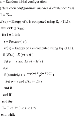
11.2.1.3 Simulated Annealing-Based Fuzzy Clustering Simulated annealing (SA) [15] is an optimization tool that has successful applications in a wide range of combinatorial optimization problems. This fact motivated researchers to use a SA to optimize the clustering problem, where it provides near optimal solutions of an objective or fitness function in the complex, large, and multimodal landscapes. In SA based fuzzy clustering [11], a string or configuration encodes K cluster centers. The fuzzy membership of all the points that are encoded in the configuration is computed by using Eq. (11.2). configuration. Subsequently, the string is updated using the new centers [Eq. (11.3)]. Thereafter, the energy function, Jm, is computed as per Eq. (11.1). The current string is perturbed using the mutation operation, as discussed for GAFC. This way, perturbation of a string yields a new string. It’s energy is also computed in a similar fashion. If the energy of the new string (E(s)) is less than that of the current string (E(p)), the new string is accepted. Otherwise, the new string is accepted based on a probability ![]() , where T is the current temperature of the SA process. Figure 11.1 demonstrates the SAFC algorithm.
, where T is the current temperature of the SA process. Figure 11.1 demonstrates the SAFC algorithm.
FIGURE 11.1 The SAFC algorithm.
11.2.2 Cluster Validity Indices
11.2.2.1I index A cluster validity index I, proposed in [16] is defined as follows:
where K is the number of clusters. Here,
and
The index I is a composition of three factors, namely, 1/K; E1/EK, and DK. The first factor will try to reduce index I as K is increased. The second factor consists of the ratio of E1, which is constant for a given data set, to EK, which decreases with an increase in K. To compute E1, the value of K in Eq. (11. ef{ek}) is taken as 1 (i.e., all the datapoints are considered to be in the same cluster). Hence, because of this term, index I increases as EK decreases. This, in turn, indicates that formation of more clusters, which are compact in nature, would be encouraged. Finally, the third factor, DK, which measures the maximum separation between two clusters over all possible pairs of clusters, will increase with the value of K. However, note that this value is upper bounded by the maximum separation between two datapoints in the data set. Thus, the three factors are found to compete with and balance each other critically. The power p is used to control the contrast between the different cluster configurations. In this chapter, p = 2.
11.2.2.2 Silhouette Index The silhouette index [17] is a cluster validity index that is used to judge the quality of any clustering solution C. Suppose a represents the average distance of a datapoint from the other datapoints of the cluster to which the datapoint is assigned, and b represents the minimum of the average distances of the datapoint from the datapoints of the other clusters. Now, the silhouette width s of the datapoint is defined as
Silhouette index s(C) is the average silhouette width of all the datapoints and reflects the compactness and separation of clusters. The value of the silhouette index varies from −1 to 1, and higher values indicate a better clustering result.
11.3 DIFFERENTIAL EVOLUTION BASED FUZZY CLUSTERING
11.3.1 Vector Representation and Population Initialization
Each vector is a sequence of real numbers representing the K cluster centers. For an N− dimensional space, the length of a vector is l = N × K, where the first N positions represent the first cluster center. The next N positions represent those of the second cluster center, and so on. The K cluster centers encoded in each vector are initialized to K randomly chosen points from the data set. This process is repeated for each of the P vectors in the population, where P is the size of the population.
11.3.2 Fitness Computation
The fitness of each vector (Jm) is computed using Eq. (11.1). Subsequently, the centers encoded in a vector are updated using Eq. (11.3).
11.3.3 Mutation
The it h individual vector of the population at time-step (generation) t has l components, that is,
For each target vector Gi,l(t) that belongs to the current population, DE samples three other individuals, like Gx,l(t), Gy,l(t), and Gz,l(t) (as describe earlier) from the same generation. Then, the (componentwise) difference is calculated, scale by a scalar F (usually ![]() [0, 1]), and creates a mutant offspring ϑi,l(t + 1).
[0, 1]), and creates a mutant offspring ϑi,l(t + 1).
11.3.4 Crossover
In order to increase the diversity of the perturbed parameter vectors, crossover is introduced. To this end, the trial vector:
is formed, where

In Eq. (11.11), randl(0,1) is the lt h evaluation of a uniform random number generator with outcome ![]() [0, 1], CR is the crossover constant
[0, 1], CR is the crossover constant ![]() [0, 1] that has to be determined by the user. rand(i) is a randomly chosen index
[0, 1] that has to be determined by the user. rand(i) is a randomly chosen index ![]() 1, 2,…,l that ensures that Ui,l(t+1) gets at least one parameter from ϑi,l(t+1).
1, 2,…,l that ensures that Ui,l(t+1) gets at least one parameter from ϑi,l(t+1).
11.3.5 Selection
To decide whether or not it should become a member of generation G+1, the trial vector Ui,l(t+1) is compared to the target vector Gi,l(t) using the greedy criterion. If vector Ui,l(t+1) yields a smaller cost function value than Gi,l(t), then Ui,l(t+1) is set to Gi,l(t); otherwise, the old value Gi,l(t) is retained.
11.3.6 Termination Criterion
The processes of mutation, crossover, and selection are executed for a fixed number of iterations. The best vector seen up to the last generation provides the solution to the clustering problem.
11.4 EXPERIMENTAL RESULTS
11.4.1 Gene Expression Data Sets
11.4.1.1 Yeast Sporulation This data set [18] consists of 6118 genes measured across seven time points (0, 0.5, 2, 5, 7, 9, and 11.5 h) during the sporulation process of budding yeast. The data are then log-transformed. The sporulation data set is publicly available at the website http://cmgm.stanford.edu/pbrown/sporulation. Among the 6118 genes, the genes whose expression levels did not change significantly during the harvesting have been ignored from further analysis. This is determined with a threshold level of 1.6 for the root mean squares of the log2-transformed ratios. The resulting set consists of 474 genes.
11.4.1.2 Yeast Cell Cycle The yeast cell cycle data set was extracted from a data set that shows the fluctuation of expression levels of ∼6 000 genes over two cell cycles (17 time points). Out of these 6000 genes, 384 genes have been selected to be cell-cycle regulated [19]. This data set is publicly available at http://faculty.washington.edu/kayee/cluster.
11.4.1.3 Arabidopsis Thaliana This data set consists of expression levels of 138 genes of Arabidopsis Thaliana. It contains expression levels of the genes over eight time points, namely, 15, 30, 60, 90 min, 3, 6, 9, and 24 h [20]. It is available at http://homes.esat.kuleuven.be/thijs/Work/Clustering.html.
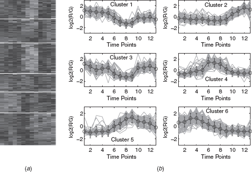
11.4.1.4 Human Fibroblasts Serum This data set [21] contains the expression levels of 8613 human genes. This data set has 13 dimensions corresponding to 12 time points (0, 0.25, 0.5, 1, 2, 4, 6, 8, 12, 16, 20, and 24 h) and one unsynchronized sample. A subset of 517 genes whose expression levels changed substantially across the time points have been chosen. The data is then log2-transformed. This data set is available at http://www.sciencemag.org/feature/data/984559.shl.
All the data sets are normalized so that each row has mean 0 and variance 1.
11.4.2 Performance Metrics
For evaluating the performance of the clustering algorithms, Jm [12], I [16], and the silhouette index s(C) [17] are used for four real-life gene expression data sets, respectively. Also, two cluster visualization tools, namely, Eisen plot and cluster profile plot, have been utilized.
11.4.2.1 Eisen Plot In Eisen plot [22] [e.g., Fig. 11.2(a) ], the expression value of a gene at a specific time point is represented by coloring the corresponding cell of the data matrix with a color similar to the original color of its spot on the microarray. The shades of red represent higher expression levels, the shades of green represent lower expression levels, and the colors toward black represent absence of differential expression. In our representation, the genes are ordered before plotting so that the genes that belong to the same cluster are placed one after another. The cluster boundaries are identified by white colored blank rows.
FIGURE 11.2 Yeast sporulation data clustered using the DEFC–SVM clustering method. (a) Eisen plot and (b) cluster profile plots.

11.4.2.2 Cluster Profile Plot The cluster profile plot [e.g., Fig. 11.2(b) ] shows the normalized gene expression values (light green) for each cluster of the genes of that cluster with respect to the time points. Also, the average expression values of the genes of a cluster over different time points are plotted as a black line together with the standard deviation within the cluster at each time point.
11.4.3 Input Parameters
The population size and number of generation used for DEFC, GAFC, SAFC algorithms are 20 and 100, respectively. The crossover probability (CR) and mutation factors (F) used for DEFC is taken to be 0.7 and 0.8, respectively. The crossover and mutation probabilities used for GAFC are taken to be 0.8 and 0.3, respectively. The parameters of the SA based fuzzy clustering algorithm are as follows: Tmax = 100, Tmin = 0.01, r = 0.9, and k = 100. The FCM algorithm is executed till it converges to the final solution. Note that the input parameters used here are fixed either following the literature or experimentally. For example, the value of fuzzy exponent (m), the scheduling of simulated annealing follows the literature, whereas the crossover, mutation probability, population size, and number of generation is fixed experimentally. The number of clusters for the sporulation, cell cycle, arabidopsis, and serum data sets are taken as 6, 5, 4, and 6, respectively. This conforms to the findings in the literature [18–2].
11.4.4 Results
Table 11.1 reports the average values of Jm, I, and s(C) indices provided by DEFC, GAFC, SAFC, and FCM clustering of > 5 0 runs of the algorithms for the four real-life data sets considered here. The values reported in the tables show that for all the data sets, DEFC provides the best Jm, I, and s(C) index score. For example, for the yeast sporulation data set, the average value of s(C) produces by the DEFC algorithm is 0.5591. The s(C) value produced by GAFC, SAFC and FCM are 0.5421, 0.5372, and 0.5163, respectively. Figures 11.3 and 11.4 demonstrate the boxplot as well as the convergence plot of different algorithms. However, the performance of the proposed DEFC is best for all the data sets.
TABLE 11.1 Average Jm, I, and s(C) Index Values of > 50 Runs of Different Algorithms for the Four Gene Expression Data Sets
FIGURE 11.3 Boxplot of s(C) for different clustering algorithms on (a) yeast sporulation, (b) yeast cell cycle, (c) Arabidopsis Thaliana, and (d) human fibroblasts serum.
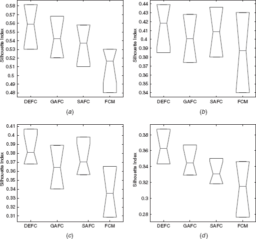
FIGURE 11.4 Convergence plot of different clustering algorithms on (a) yeast sporulation, (b) yeast cell cycle, (c) Arabidopsis Thaliana, and (d) human fibroblasts serum.

11.5 INTEGRATED FUZZY CLUSTERING WITH SUPPORT VECTOR MACHINES
11.5.1 Support Vector Machines
Support vector machines (SVM) is a learning algorithm originally developed by Vapnik (1995). The SVM classifier is inspired by statistical learning theory and they perform structural risk minimization on a nested set structure of separating hyperplanes cite{eisen98}. Viewing the input data as two sets of vectors in d− dimensional space, an SVM constructs a separating hyperplane in that space, one that maximizes the margin between the two classes of points. To compute the margin, two parallel hyperplanes are constructed on each side of the separating one, which are “pushed up against”’ the two classes of points. Intuitively, a good separation is achieved by the hyperplane that has the largest distance to the neighboring datapoints of both classes. The larger margins or distances between these parallel hyperplanes indicate a better generalization error of the classifier. Fundamentally, the SVM classifier is designed for two-class problems. It can be extended to handle multiclass problems by designing a number of one-against-all or one-against-one two-class SVMs. For example, a K− class problem is handled with K two-class SVMs.
For linearly nonseparable problems, SVM transforms the input data into a very high-dimensional feature space, and then employs a linear hyperplane for classification. Introduction of a feature space creates a computationally intractable problem. The SVM handle this by defining appropriate kernels so that the problem can be solved in the input space itself. The problem of maximizing the margin can be reduced to the solution of a convex quadratic optimization problem, which has a unique global minimum.
We consider a binary classification training data problem. Suppose a data set consists of n feature vectors < xi, yi >, where yi ![]() {+1,−1} denotes the class label for the datapoint xi. The problem of finding the weight vector w can be formulated as minimizing the following function:
{+1,−1} denotes the class label for the datapoint xi. The problem of finding the weight vector w can be formulated as minimizing the following function:
subject to
Here, b is the bias and the function Ф(x) maps the input vector to the feature vector. The SVM classifier for the case on linearly inseparable data is given by
Where, K is the kernel matrix and n is the number of input patterns having nonzero values of the Langrangian multipliers(βi). In case of categorical data, xi is the it h sample, and yi is the class label. These n input patterns are called support vectors, and hence the name support vector machines. The Langrangian multipliers(βi) can be obtained by maximizing the following:
subject to
Where, C is the cost parameter, which controls the number of nonseparable points. Increasing C will increase the number of support vectors, thus allowing fewer errors, but making the boundary separating the two classes more complex. On the other hand, a low value of C allows more nonseparable points, and therefore, has a simpler boundary. Only a small fraction of the βi coefficients are nonzero. The corresponding pairs of xi entries are known as support vectors and they fully define the decision function. Geometrically, the support vectors are the points lying near the separating hyperplane, where K(xi, xj) = Ф(xi).Ф(xj) is called the kernel function. The kernel function may be linear or nonlinear, like polynomial, sigmoidal, radial basis functions (RBF), and soon. The RBF kernels are of the following form:
where xi denotes the it h datapoint and w is the weight. In this chapter, the above mentioned RBF kernel is used. Also, the extended version of the two-class SVM that deals with the multiclass classification problem by designing a number of one-against-all two-class SVMs, is used here.
11.5.2 Improving Fuzzy Clustering with SVM
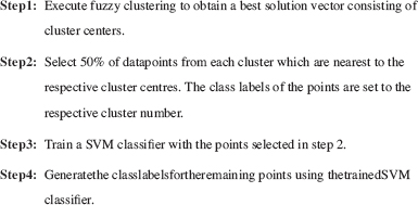
This section describes the developed scheme for combining the fuzzy clustering algorithm (DEFC, GAFC, SAFC, or FCM) described in Sections 11.2 and 11.3 with the SVM classifier. This is motivated due to the fact that the presence of training points, supervised classification usually performs better than the unsupervised classification or clustering. In this chapter, we have exploited this advantage while selecting some training points using the differential evolution-based fuzzy clustering technique and the concept of proximity of the points from the respective cluster centers. The basic steps are described in Figure 11.5.
FIGURE 11.5 Algorithm of integrated fuzzy clusteing with SVM.
11.5.3 Results
Table 11.2 show the results in terms of s(C) obtained by the integrated clustering algorithm for the four gene expression data sets, respectively. It can be seen from this table that irrespective of the clustering method used in the developed algorithm, the performance gets improved after the application of SVM. For example, in the case of yeast sporulation, the s(C) values produced by DEAFC is 0.5591 while this gets improved to 0.5797 when SVM is used. A similar result is found for another data set also. The results demonstrate the utility of adopting the approach presented in this paper, irrespective of the clustering method used.
TABLE 11.2 Average Values of s(C) for the Integrated Fuzzy Clustering Algorithm Over 50 runs
To demonstrate visually the result of DEFC–SVM clustering, Figures 11.2, 11.6–11.8 show the Eisen plot and cluster profile plots provided by DEFC–SVM on the two data sets, respectively. For example, the six clusters of the yeast sporulation data are very prominent, as shown in the Eisen plot [Fig. 11.2(a) ]. It is evident from this figure that the expression profiles of the genes of a cluster are similar to each other and produce similar color patterns. The cluster profile plots [Fig. 11.2(b) ] also demonstrate how the expression profiles for the different groups of genes differ from each other, while the profiles within a group are reasonably similar. A similar result is obtained for the other data set.
FIGURE 11.6 Yeast cell cycle data clustered using the DEFC–SVM clustering method. (a) Eisen plot and (b) cluster profile plots.
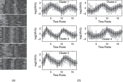
FIGURE 11.7 Arabidopsis Thaliana data clustered using the DEFC–SVM clustering method. (a) Eisen plot and (b) Cluster profile plots.
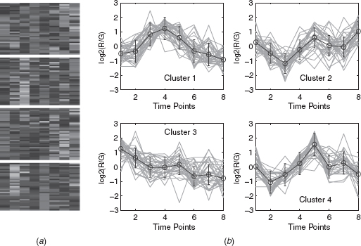
FIGURE 11.8 Human fibroblasts serum data clustered using the DEFC–SVM clustering method. (a) Eisen plot and (b) Cluster profile plots.
11.5.4 Biological Significance
The biological relevance of a cluster can be verified based on the statistically significant gene ontology (GO) annotation database (http://db.yeastgenome.org/cgi-bin/GO/goTermFinder). This is used to test the functional enrichment of a group of genes in terms of three structured, controlled vocabularies (ontologies), namely, associated biological processes, molecular functions, and biological components. The degree of functional enrichment (p-value) is computed using a cumulative hypergeometric distribution. This measures the probability of finding the number of genes involved in a given GO term (i.e., process, function, and component) within a cluster. From a given GO category, the probability p of getting k or more genes within a cluster of size n, can be defined as [23]:
where f and g denote the total number of genes within a category and within the genome, respectively. Statistical significance is evaluated for the genes in a cluster by computing the p-value for each GO category. This signifies how well the genes in the cluster match with the different GO categories. If the majority of genes in a cluster have the same biological function, then it is unlikely that this takes place by chance and the p-value of the category will be close to 0.
The biological significance test for yeast sporulation data has been conducted at the 1% significance level. For different algorithms, the number of clusters for which the most significant GO terms have a p-value < 0.01 (1% significance level) are as follows: DEFC - 6, GAFC - 6, SAFC - 6, and FCM - 6. Table 11.3 reports the three most significant GO terms (along with the corresponding p-values) shared by the genes of each of the six clusters identified by the DEFC technique (Fig. 11.2). As is evident from the table, all the clusters produced by DEFC clustering scheme are significantly enriched with some GO categories, since all the p-values are < 0.01 (1% significance level). This establishes that the developed DEFC clustering scheme is able to produce biologically relevant and functionally enriched clusters.
TABLE 11.3 The Three Most Significant GO Terms and the Corresponding p-Values for Each of the Six Clusters of Yeast Sporulation Data as Found by the IDEFC Clustering Technique

11.6 CONCLUSION
In this chapter, a differential evolution-based fuzzy clustering technique has been described for the analysis of microarry gene expression data sets. The problem of fuzzy clustering has been modeled as one of optimization of a cluster validity measure. Results on different gene expression date sets indicate that DEFC consistently performs better than GAFC, SAFC, and FCM clustering techniques. To improve the performance of clustering further, a SVM classifier is trained with a fraction of gene expression datapoints selected from each cluster based on the proximity to the respective cluster centers. Subsequently, the remaining gene expression datapoints are reassigned using the trained SVM classifier. Experimental results indicate that this approach is likely to yield better results irrespective of the actual clustering technique adopted.
As a scope of further research, the use of kernel functions other than RBF may be studied. A sensitivity analysis of the developed technique with respect to different setting of the parameters, including the fraction of the points to be used for training the SVM, needs to be carried out. Moreover, the DE based algorithm can be extended in the multiobject framework and the results need to be compared with other related techniques [12,20].
REFERENCES
1. S. Bandyopadhyay, U. Maulik, and J. T. Wang (2007), Analysis of Biological Data: A Soft Computing Approach. World Scientific, NY.
2. B. S. Everitt (1993), Cluster Analysis, 3rd ed., Halsted Press, NY.
3. J. A. Hartigan (1975), Clustering Algorithms, Wiley, NY.
4. A. K. Jain and R. C. Dubes (1988), Algorithms for Clustering Data, Prentice-Hall, Englewood Cliffs, NJ.
5. R. Storn and K. Price (1995), Differential evolution—{A} simple and efficient adaptive scheme for global optimization over continuous spaces, Tech. Rep. TR-95-012, International Computer Science Institute, Berkley.
6. K. Price, R. Storn, and J. Lampinen (2005), Differential Evolution—{A} Practical Approach to Global Optimization, Springer, Berlin.
7. R. Storn and K. Price (1997), Differential evolution—{A} simple and efficient heuristic strategy for global optimization over continuous spaces, J. Global Opt., 11:341–359.
8. A. Zilinska and A. Zhigljavsky (2008), Stochastic global optimization, Springer, NY.
9. M. Omran, A. Engelbrecht, and A. Salman (2005), Differential evolution methods for unsupervised image classification, Proc. IEEE Int. Conf. Evol. Comput., 2:966–973.
10. M. K. Pakhira, S. Bandyopadhyay, and U. Maulik (2005), A study of some fuzzy cluster validity indices, genetic clustering and application to pixel classification, Fuzzy Sets Systems, 155:191–214.
11. S. Bandyopadhyay (2005), Simulated annealing using a reversible jump markov chain monte carlo algorithm for fuzzy clustering, IEEE Trans. Knowledge Data Eng., 17(4):479–490.
12. J. C. Bezdek (1981), Pattern Recognition with Fuzzy Objective Function Algorithms, Plenum, New York.
13. D. E. Goldberg (1989), Genetic Algorithms in {S}earch, Optimization and Machine Learning, Addison-Wesley, NY.
14. U. Maulik and S. Bandyopadhyay (2000), Genetic algorithm based clustering technique, Pattern Recognition, 33:1455–1465.
15. S. Kirkpatrik, C. D. Gelatt, and M. P. Vecchi (1983), Optimization by simulated annealing, Science, 220:671–680.
16. U. Maulik and S. Bandyopadhyay (2002), Performance evaluation of some clustering algorithms and validity indices, IEEE Trans. Pattern Anal. Machine Intelligence, 24(12):1650–1654.
17. P. J. Rousseeuw (1987), Silhouettes: a graphical aid to the interpretation and validation of cluster analysis, J. Compt. App. Math, 20:53–65.
18. S. Chu, J. DeRisi, M. Eisen, J. Mulholland, D. Botstein, P. O. Brown, and I. Herskowitz (1998), The transcriptional program of sporulation in budding yeast, Science, 282:699–705.
19. R. J. Cho et al. (1998), A genome-wide transcriptional analysis of mitotic cell cycle, Mol. Cell., 2:65–73.
20. P. Reymonda, H. Webera, M. Damonda, and E. E. Farmera (2000), Differential gene expression in response to mechanical wounding and insect feeding in arabidopsis, Plant Cell., 12:707–720.
21. V. R. Iyer, M. B. Eisen, D. T. Ross, G. Schuler, T. Moore, J. Lee, J. M. Trent, L. M. Staudt, J. J. Hudson, M. S. Boguski, D. Lashkari, D. Shalon, D. Botstein, and P. O. Brown (1999), The transcriptional program in the response of the human fibroblasts to serum, Science, 283:83–87.
22. M. B. Eisen, P. T. Spellman, P. O. Brown, and D. Botstein (1998), Cluster analysis and display og genome-wide expression patterns. Proc. Nato. Acad. Scie. USA, pp. 14863–14868.
23. S. Tavazoie, J. Hughes, M. Campbell, R. Cho, and G. Church (1999), Systematic determination of genetic network architecture, Nature Genet., 22:281–285.
24. V. Vapnik (1998), Statistical Learning Theory, John Wiley & Sons, Inc., NY.