CHAPTER 16

ANALYZING TOPOLOGICAL PROPERTIES OF PROTEIN–PROTEIN INTERACTION NETWORKS: A PERSPECTIVE TOWARD SYSTEMS BIOLOGY

MALAY BHATTACHARYYA AND SANGHAMITRA BANDYOPADHYAY

16.1 INTRODUCTION

Biological systems are too complex to be represented with a stand-alone computational model [1,2]. The intricacies involved in the genomic or proteomic level of an organism, even in one of the simplest (e.g., amoeba), is hard to replicate. In spite of the complexities involved in the biological systems, they abide by a set of protocols [3]. The systematic study of such complex protocols in biological systems is the main concern in systems biology. In an analytical view, systems biology cares about the emergence of phenotypic characteristics from the genotypes and figures out the protocols behind the response to alterations of these characteristics in the environment or in the system components.

Many high-throughput technologies evolved in recent decades have enabled the analysis of various properties of the transcriptome and proteome of several organisms. These properties are occasionally mapped to an interaction network structure [4]. The identification of significant modules of genes and proteins, which have a high degree of association with each other in these networks, can add potentials to this direction of research. Individual or combined mining of gene and protein cointeraction networks is a nascent area of research that has seen promise through such module-specific studies [5–7]. A set of genes has a high chance of participating in a common biological pathway if they form a module in both the gene–gene and protein–protein interaction networks (PPINs). Sometimes, these networks are constructed by combining multiple sources of information by way of investigating associations between them [8–10]. Thus, we can obtain a robust and integrated view of the underlying biology. However, one of the most notable properties of these biological networks explored very recently is the whimsical dynamic behavior they exhibit corresponding to the network parameters [11]. Surprisingly, the dynamics produced by these networks are in some way more reliant on the network topology. Therefore, biological network analysis at the topological level is undeniably an important direction of research in systems biology.

In the perspective of systems biology, a biological organization has several levels of abstraction, namely, genomic, proteomic, and cellular level, and so on. Unveiling the interdependencies and intradependencies of the components in these levels is a major challenge in systems biology. Of these levels of abstraction in a biological system, the proteomic level acts as the dominant functional bridge between the others. Proteins are essential components in a living being. What a protein does and how it works defines the comprehensive activity within an organism. With the availability of a large volume of protein level interaction information of various organisms from multiple sources, a new challenge has been brought into the postgenomic era of elucidating the cellular level protein functions. Unveiling the comprehensive protein interactome of an organism provides a framework for understanding biology as an integrated system [12]. Protein–protein interaction (PPI) information provides a local as well as a global view of the interaction modules of proteins participating in significant similar activities. Essentially, such PPI information can be obtained via biological studies (X-ray crystallography, yeast two-hybrid, mass spectrometry, etc.) [13] or can be predicted in silico (hidden Marcov model, neural network, random forest, etc.) [14]. This chapter focuses exclusively on the topological properties of interaction networks of proteins and their significance in the systems level. Instead of pursuing a piecemeal study of the single components, we pay attention to the more global analyzes of the structure, function, and dynamics of the networks in which macromolecules work [12].

This chapter is organized as follows: In Section 16.2, we discuss various topological properties and structures of interaction networks. In Section 16.3, the details on state-of-the-art knowledge on the topology-based analysis of PPINs are provided. The problem is presented formally with necessary precursory details are in Section 16.4. Sections 16.5–16.6 include the algorithmic approach to the problem and its theoretical background. In Section 16.7, the empirical analysis along with the concern of system level study is provided on the structures explored from the studied PPIN. Finally, Section 16.8 concludes this chapter.

16.2 TOPOLOGY OF PPI NETWORKS

A network N = (V,A) is defined with a set of nodes and a set of arcs connecting these nodes. Generally, we discard self-loops or parallel arcs from a simple network and consider it to be undirected. Whenever a network is called directed, we distinguish between the two arcs . A subnetwork N′ = (V′,A′) is a part of the network N = (V,A), such that V′ V and A′ A. Again, by the term induced subnetwork we restrict A′ to include only the comprehensive set of arcs existing within the nodes of V′ in N. A weighted network, N = (V,A,W), is defined with a set of nodes V, a set of arcs A, and a weight function W defined over the set of arcs, such that W : A → .

A PPIN is a symbolization of PPIs in the form of a network. A PPIN is defined by a doublet , where P denotes the set of proteins and denotes the set of interactions. So, the set P is equivalent to V, and I is equivalent to A. Frequently, a PPIN is generalized using a triplet representation is a weight function mapping each interaction to a positive real value. These weights are used to rank the significance of the interactions between protein pairs [9]. A PPIN is called weighted or unweighted (sometimes termed as binary), depending on the inclusion or exclusion of the weight function W. In the course of study presented in this chapter, undirected and weighted PPINs will be studied throughout. Let us suppose that |S| represents the cardinality of a set S and the other notations are customary, unless specified otherwise.

The physical or logical organization of the components (nodes, arcs, etc.) in a network is known to be its topology. Topology of a particular type of network is preserved through the contraction or expansion in its size. This section describes some of the important topological properties and structures useful for the study of biological interaction networks.

16.2.1 Topological Properties

Definition 16.2.2 (Degree [15]): The degree of a node defines the cardinality of its first-order neighborhood set (i.e., the number of arcs connected to it).

In a directed network, the degree of a node can be separated into two distinct categories, namely, the in and the out degrees. The in and out degrees of a node defines the number of arcs directed to and directed from the node itself, respectively. For such networks, the total degree of a node equals the sum of its in and out degrees.

Definition 16.2.2 (Degree distribution [16]): Given a network N = (V,A), its degree distribution is defined as the probability distribution of the degree values of its nodes.

For a directed network, there could be two types of degree distributions, namely, the in degree and the out degree distributions.

Definition 16.2.3 (Clustering coefficient [17]): Given a network N = (V,A), the clustering coefficient of a node in N is defined as the frequency of arcs within the subnetwork induced by its first-order neighborhood.

By the term frequency, we mean the fraction of the existing number arcs to that of the maximum possible number of arcs. The clustering coefficient can also be defined for a subnetwork as the frequency of arcs within the subnetwork itself. The clustering coefficient of a subnetwork is sometimes defined as its density.

Definition 16.2.4 (Core clustering coefficient [18]): Given a network N = (V,A) and a parameter k, the core clustering coefficient of a node in N is defined as the clustering coefficient of the largest subnetwork of its first-order neighborhood with minimal degree k.

The core clustering coefficient, in contrast to the standard clustering coefficient, increases the weights of highly dense subnetworks while giving less weights to the small degree nodes 18].

Definition 16.2.5 (Betweenness centrality [19]): Given a network N = (V,A), the betweenness centrality of a node in N is defined by the fraction of all-pair shortest paths in N that includes the specific node.

Definition 16.2.6 (Czekanowski–Dice (CD) distance [20]): In a network N = (V,A), the CD distance between two nodes u, v V, is computed as

where N(u) denotes the first-order neighbors of u and denotes the non-neighbors of u.

The set of CD distances of all the node pairs provide important topological information about the distribution of sharing of neighborhood within a network.

Definition 16.2.7 (Scale-free property [16]): A network N = (V,A) is said to follow the scale-free property if its nodes follow a power law degree distribution [i.e, the probability P(k) that a node in N is adjacent to k other nodes, decays as a power law following P(k)∼ k-γ (γ > 0)].

Now, we describe some of the topological structures used commonly in biological network analysis in Section 16.2.2.

16.2.2 Topological Structures

Definition 16.2.8 (Clique [21]): Given a network N = (V,A), a clique is defined as a complete subnetwork of is said to be a clique if the degree of all the nodes in the subnetwork induced by K from N is (K-1)].

Clique is one of the most exercised topological structures of a biological network. It essentially represents the all-to-all association of the nodes within it, and thus, is very useful to characterize cofunctional modules. Sometimes, the stringent all-to-all association of a clique does not prove to be useful for real-life analyzes. Thus, the concept of quasi-completeness has emerged in network analysis.

Definition 16.2.9 (γ-quasi-complete network [6]): A network N = (V,A) is a γ-quasi-complete network (0 < γ ≤ 1) if every node in the network has at least degree

Definition 16.2.10 (γ-quasi-clique [6]): In a network N = (V,A), a subset of nodes V′ V forms a γ-quasi-clique (0 < γ ≤ 1) if the subnetwork induced by V′ is a γ-quasi-complete network.

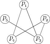
Figure 16.1 shows a 2/3–quasi-clique in a1/4-quasi-complete network. The node corresponding to the protein p5 attains the minimum degree value 1 in the network, whereas the maximum degree value was possible up to 4. So, the complete network is only 1/4-quasi-complete. But in the subnetwork induced by the proteins p1, p2, p3, p4, the minimum degree value is 2 (as the degree value is the same for all the nodes), and therefore, it is 2/3-quasicomplete. Certainly, a 1-quasi-complete network is a complete network, whereas a 1-quasi-clique is a clique.

Definition 16.2.11 (γ-quasi-biclique) [22]): In a network N = (V,A) a bipartite subnetwork N′ = (V1,V2,A) is said to be a γ-quasi-biclique (0 < γ ≤ 1) if the subnetwork induced by these two sets of nodes contains at least number of arcs.

16.3 LITERATURE SURVEY

Proteomic research is one of the early initiatives in the domains of molecular and systems biology. To date, it is one of the extensively studied domain of research. Many studies have been carried out in the last few decades on the exploration of various topological structures from biological networks with various motivations (function prediction, system level study, etc.). Exploring cliques from interaction networks is the most studied topological problem in computational biology [21,23]. Currently, we can find promising studies where maximum cliques have been merged with overlapping neighboring cliques to find dense cores in the PPIN of Escherichia coli [24]. In this study, strong correlation between cliques and essentiality of proteins have also been established by studying the PPIN of Saccharomyces cerevisiae. Such observed structure of essential cores have been found to take part in significant roles in the protein networks.

Due to the noise-prone behavior of biologically evolved data, clique finding in biological networks is a restrictive approach. Quasi-cliques are often suitable descriptors of a coherent module in biological networks. A number of studies are in the literature to explore quasi-cliques from networks. An earlier study presented a greedy randomized adaptive search procedure (GRASP) for finding the set of large quasi-cliques (for a given γ) in large networks of order >105 [25]. Here, the definition of a quasi-clique is somehow equivalent to the definition of density. However, the works carried out at that time neither found the complete set of quasi-cliques, nor addressed how to mine the largest quasi-clique. A current study proposes an efficient mining algorithm (Crochet) to explore the complete set of quasi-cliques [7]. Recently, the original algorithm has been improved (Crochet+) keeping a similar motivation of joint mining of gene and protein interaction networks [6]. Such studies are indeed significant. However, the limitation of these approaches is that they provide the complete set of maximal quasi-cliques. So, it is computationally hard to sort out the largest quasi-clique using such an approach. In a recent study, an algorithm for finding approximately largest quasi-cliques from the human PPIN has been proposed [5].

Earlier, it was shown that quasi-cliques and quasi-bicliques are able to symbolize groups of proteins associated with coherent biological activities in S. cerevisiae [26]. In several biological applications, quasi-cliques have been used to represent coherent modules, whereas, the quasi-bicliques have been used to depict the cofunctionality or coregulating nature between module pairs. Mining quasi-bicliques in such networks provides an important direction toward the study of biological pathways, protein complexes, and protein function. In [27], several quasi-cliques and quasi-bicliques were identified from the PPIN of S. cerevisiae using spectral analysis and validated using the annotation information. Again, in a later study quasi-bicliques were explored using a branch and bound method based on second-order neighborhood information [27]. In a recent study, maximum quasi-bicliques have been searched out from PPIN of S. cerevisiae using a divide and conquer approach [28]. This approach has the limitation of dependency on the selection of start splitting node, which restricts it often in reaching the global optimum.

There are several network-based prediction methods of protein functions [15]. Several works have focused solely on the functional module identification from PPI data. We describe some approaches that are based on the decomposition of the PPIN into subnetworks based on some topological properties. The molecular complex detection algorithm (MCODE) [18] is one such approach. It consists of the consecutive stages of node weighting, complex prediction, and an optional postprocessing step. This approach has motivated several successive improvements [29]. In a relatively recent study, expression similarity information (obtained from microarray data) has been integrated with topological information (obtained from high-throughput interaction data) to explore significantly connected subnetworks [4] jointly active connected subnetworks (JACS). A subnetwork is significant if it is highly connected in the interaction data, and in addition, has high average internal coherence in the corresponding gene coexpression network. These subnetworks are termed as jointly active connected subnetworks JACS. The algorithm proposed in this work, MATISSE [4], explores JACS by the successive steps of initializing dense subnetworks (seed) by enumeration, expansion of the seed, and filtering based on their significance. Again, the limitation of this approach lies in the prerequisite of network connectivity that is influenced by the high rate of false-negative interactions.

Literature studies strongly emphasize that the locally dense regions (cliques–quasi-cliques–subnetworks) of an interaction network represent protein complexes. However, defining density in the locality of PPINs is itself a dynamic concept. Several possible interpretations of dense regions are in existence and they mostly differ from the motivation with which they are used. A k-core is a maximal subnetwork such that each node in the subnetwork has at least degree k. A k-plex is a subnetwork such that each node in the subnetwork has at least degree (O(N)-k), where O(N) is the order of the subnetwork. A k-block is a maximal subnetwork such that each pair of nodes in the subnetwork is connected by k node-disjoint paths. An n-clan is a subnetwork such that the distance between any two nodes is less than or equal to n for paths within the subnetwork. These are some of the different representations of dense regions (protein complexes) that are currently emerging in use for interaction network analysis [30]. Here, we propose a heuristic algorithm to find the largest dense k-subnetwork in large scale-free networks that are sparse. We construct a PPIN, by integrating multiple topological properties, that is both sparse and scale-free. Finally, we explore our defined dense protein modules (dense k-subnetworks) by mining the network. The way we define a dense region in a weighted human PPIN is promising. Again, this kind of approach is novel in the perspective of systems biology.

16.4 PROBLEM DISCUSSION

Suppose, a set of proteins and their corresponding PPIN is provided. Here, we address the problem of searching the largest PPI modules that have a high degree of association therein. First, the problem is given formally accompanying the necessary precursory details. Then, the method of mining is presented in the later sections.

Definition 16.4.1 (k-subnetwork of a weighted network): A k-subnetwork of any arbitrary weighted network, N = (V,A,W), denoted by Vk, is defined as an induced subnetwork of N of order

Definition 16.4.2 (Association density of a node): Given a weighted network N = (V,A,W), the association density of a node vi V with respect to a k-subnetwork , is defined as the ratio of the sum of the arc weights between vi and each of the nodes belonging to Vk, and the cardinality of the set Vk. The association density of a node vi with respect to the k-subnetwork Vk is computed as

where Wvivj denotes the weight of the arc (vi,vj).

Definition 16.4.3 (Dense node): We call a node vi within a k-subnetwork Vk, dense with respect to an association density threshold δ, if

Definition 16.4.4 (Association density of a k-subnetwork): The association density of a k-subnetwork, Vk, is defined as the minimum of the association densities of all the nodes in it with respect to the remaining (k-1)-subnetworks. So, the association density of a k-subnetwork Vk is given by

Definition 16.4.5 (Dense k-subnetwork): We call a k-subnetwork, Vk, dense with respect to an association density threshold δ if .

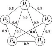
As mentioned in Section 16.2, the density of a network–subnetwork is defined as the ratio of the total number of arcs existing in and the maximum number of arcs that could possibly appear within them. Thus, it may so happen that a k-subnetwork becomes dense although it contains some low degree values. In the network shown in Figure 16.2, the density of the k-subnetwork , in the conventional sense, is 4.5/6. However, it is evident that the association of the node p5 is poor as it has very low connectivity with the other nodes. A dense association should not only satisfy a high overall density, but also a high participation density of each member. Earlier studies also suggest that the computation of dense clusters should include some minimum density threshold for each node [31]. So, the concept of minimum association density threshold (a cutoff participation factor) has been included in Definition (16.4.4). Now, we present the problem of finding the largest dense k-subnetwork in a PPIN formally.

Problem Statement Given a weighted PPIN, , and an association density threshold of a k-subnetwork δ, locate a dense k-subnetwork Pkmax in ρ that has the maximum cardinality, that is, .

16.5 THEORETICAL ANALYSIS

As in this chapter, we are focusing on PPINs and they are generally found to follow the scale-free property [5]. We will concentrate on this special type of network to explore the largest dense k-subnetworks. In this regard, some theoretical analysis has been covered to devise the final algorithm.

Suppose N = (V,A) is an arbitrary undirected and connected scale-free network with decay constant γ (γ > 0). Thus, the probability P(k) that a node in N is adjacent to other nodes, decays as a power law following P(k)∼ k-γ. Evidently, this probability distribution of the discrete degree function adjoins the additional constraint . In this case P(0) = 0, as we have assumed the network N to be connected. Let the probability with which the arcs occur in N be p(N) and the probability with which an arbitrary node v attaches with the other nodes be p(v). Then, we have the following theorem:

Theorem 16.5.1 Given, p(N) and p(v) for any arbitrary network N and for a node v within it, the probability with which v will appear in a clique selected randomly from N is given as

Proof Suppose,C(k) denotes the set of all the cliques in N of size k. Then, the probability that a k-subnetwork (a subnetwork with k nodes), Vk, selected randomly from N will be inC(k), if it contains v, is given by

The probability with which the node v will always belong to the setC(k) can be computed using Eq. (16. ef{probability}) as the conditional probability

Let, vmax be the node having the highest degree value in N, and consequently, p(vmax) be the probability with which it connects the other nodes. Then, we have

Evidently, the probability value produced in Eq. (16.5) becomes higher with the increasing value of . In the case of scale-free networks, the probability with which the arcs occur (p(N)) rests at a very low value due to the scale-free degree distribution. Thus, the nodes having comparatively higher degree values have a higher probability to be selected in the largest dense k-subnetwork. Therefore, selecting the nodes with higher association density values and merging them heuristically might produce better approximation in the final result. Being inspired from the aforementioned probabilistic intuition, we now discuss the solution methodology in Section 16.6.

16.6 ALGORITHMIC APPROACH

The problem addressed here belongs to the NP complexity class. For this reason, it cannot be solved deterministically in polynomial time, unless P = NP [32]. Considering this, a heuristic solution method for providing an approximate solution of the problem has been presented in the following algorithm:

Algorithm A heuristic solution approach for the problem

Input: A weighted PPIN ρ = (P,I,W) and an association density threshold δ.

Output: The largest k-subnetwork Pkmax in ρ satisfying the association density threshold δ.

Steps of the algorithm:

We reproduce the algorithm proposed in [33] with nominal modification. In the beginning (step 1), a linked list is prepared for each protein pi P, which contains all the remaining proteins, in the order of their descending weights with respect to the corresponding protein pi. This is basically a neighboring list of proteins in the order of closeness. After this (step 2), the protein that can associate the largest number of proteins with it satisfying the association density threshold is determined. In case of a tie, it is selected randomly, and finally is used to initialize the largest k-subnetwork, Pkmax (step 3). Construction of the largest k-subnetwork then proceeds following steps 4–9. To start with, a connector list is prepared from the list of neighboring proteins of pmax, taken from the NList(pmax) (step 4). Then, the first member of the connector list is attached with the current dense k-subnetwork, Pkmax (step 6). This is in fact the closest neighbor of pmax and thus most similar in terms of the interaction weight. Thereafter, the connector list of Pkmax is updated by taking a weighted aggregation of the current connector list of Pkmax, contained in Connector and NList(Connector(1)), the corresponding NList entry of Connector(1) (step 8). The weights in this aggregation depends on the cardinalities of the two sets Pkmax [before the attachment of the protein in Connector(1)] and Connector(1) itself. Certainly, the former one is of size (kmax-1), whereas the later one is a singleton set. The iterative process continues (steps 5–9) till either all the proteins are included in Pkmax or it falls short of the association density threshold δ.

16.7 EMPIRICAL ANALYSIS

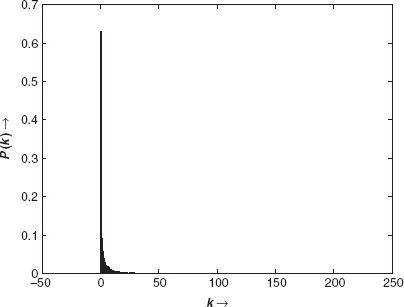
We have carried out the experimental analysis both in the directions of mining the interaction networks and verifying the significance of the protein sets explored (within the largest k-subnetworks) through a biological perspective. In order to prepare the basic interaction network, PPI information of Homo Sapiens has been collected from the Human Protein Reference Database (HPRD) [34]. The version of interaction data we have collected reports 37,107 interactions between 25,661 human proteins. The clustering coefficient of the entire network is ∼ 1.13E-4 [5]. So, the network is prominently a sparse one. To visualize the degree distribution in this network, we have plotted the probability of attachment of the nodes against their degree values, that is,P(k) denotes the probability of any arbitrary node of having a degree value of k. Scale-free degree distribution is observed in the PPIN employed in this study [16]. This is shown in Figure 16.3.

We have incorporated a novel method of integration in this topological study. Two kinds of topological information, the interaction between protein pairs and the sharing of first-order neighborhood between protein pairs, have been employed to build up a unified framework for the topological structure analysis. First, a PPIN ρ = (P,I,W) has been constructed from the up-to-date data collected from HPRD resource. Second, the sharing of first-order neighborhood information of every protein pair has been computed using the SimCD measure (inspired from the {CD} distance) to construct a separate network ρCD = (P,ICD,WCD). Recently, some existing approaches have established the usefulness of accounting the common interacting partners between two proteins as an estimate of their functional similarity [20]. This SimCD is said to be the {CD} similarity and is computed between two proteins p1, p2 P using the following final equation:

Certainly, we have . Therefore, ρCD is a weighted network, whereas in the former one, constructed from the HPRD data, ρ, is a binary network. Finally, these two networks are combined to produce an integrated network ρ+ = (P,I+,W+), where the weight function is defined as W+ = 0.5∗(W+WCD). For those interactions absent in I in the network ρ, we assume a weight of zero. Thus, ρ+ becomes a weighted and complete undirected network.

On constructing the integrated network ρ+ for the topological study, we have applied the algorithm described in Section 16.6 to investigate the largest dense k-subnetworks. We have set the association density threshold to δ = 0.55. Fixation of δ to this value has been done to ensure that for any protein pair p1,p2, (Wp1p2 + WCDp1p2) is at least 1.1. Because both of the weight functions W and WCD have an upper bound of 1, the tuning of δ to 0.55 will confirm that none of these are individually zero for any protein pair. Thus, we can make it certain that the protein pairs selected within the dense k-subnetwork have prior interaction support, and as well, prior support of sharing a common neighborhood.

By applying the algorithm on the final network, we have obtained the largest dense k-subnetwork (with respect to δ=0.55) to contain 11 proteins. The biological analysis of this protein module is provided in the following sections. We have validated the functional significance of the protein set using the resource of HPRD [34] and a functional enrichment tool FatiGO [35].

16.7.1 Gene Ontology Studies from HPRD

The information regarding the biological process, molecular function, and molecular class (cellular component) of the genes (corresponding to the proteins found in the k-subnetwork) collected from the HPRD provides an insight into the system level participation of these proteins. We have accumulated the participation of the proteins found in the largest k-subnetwork in these three categories of gene ontology. Complete information is listed in Tables 16.1–16.3. As seen from Table 16.1, four proteins, namely, ALDH1A1, APEH, FDX1, and ALDOA are responsible for the biological process of metabolism (and often for the energy pathways) and their corresponding molecular functions (observe in Table 16.2) are related to the activities of aldehyde dehydrogenase, hydrolase, oxidoreductase, and lyase, respectively. In fact, these four proteins are separate enzymes (see Table 16.3) associated with the common biological activity of metabolism. Enzymes act as catalysts for many of the biochemical reactions organized within an organism. Usually, these enzymes are very specific to a certain biochemical reaction [36]. In this regard, the four enzymes detected by the algorithm within the module are very significant. Similarly, from Table 16.1, we can identify the two proteins ADORA2A and ARF3, both of which are associated with the common tasks of cell communication and signal transduction, and again from Table 16.3 the later one is found to be a G protein, whereas the former one is its receptor. These results, obtained by combining the information provided in the Tables 16.1–16.3 suggest that the explored dense k-subnetwork is indeed a strongly coherent module of proteins. In Section 16.7.2, we produce the functional enrichment result produced from the tool FatiGO [35].

TABLE 16.1 Biological Involvement of the Proteins Found in the Largest k-Subnetwork as Annotated from the Biological Process Information

TABLE 16.2 Biological Involvement of the Proteins Found in the Largest k-Subnetwork as Annotated from the Molecular Function Information

TABLE 16.3 Biological Involvement of the Proteins Found in the Largest k-Subnetwork as Annotated from the Molecular Class (Cellular Component) Information

16.7.2 Study of Functional Enrichment with FatiGO

We have prepared two protein sets for the analysis using FatiGO. The first is a reference set, containing the 11 proteins found in the largest dense k-subnetwork, and the other one is a background set, containing the 25,650 proteins remaining after mining in the initial interaction network. We have performed a two-tailed statistical test by removing the duplicates from the protein sets using the tool FatiGO [35]. The significant terms found in the functional enrichment test are provided in Table 16.4.

TABLE 16.4 Significant GO Terms Found in the Biological Process to be Associated with the Proteins Found in the Largest k-Subnetwork

As observed in Table 16.4, the three proteins (ADORA2A, SAA1, and CD59) explored in the module are associated with the activities of coagulation, regulation of body fluids, and response to external stimulus with very low p-values. Going into a deeper analysis, it is found that these three proteins are responsible for blood coagulation. This finding is significant in the sense that <1% of the total proteins in the human protein set are related with this kind of biological activity. The p-value of this observation is as low as the order of 1E-05. From the analysis of HPRD repositories, as shown in Table 16.2, we have identified that the activities of the two proteins SAA1 and CD59 are in the form of transporter and receptor in immune response. Thus, they are responding to the immune system by participating in the blood coagulation along with the protein ADORA2A. As a whole, we have obtained six significant GO terms in the category biological process. In all of these cases, >89% of the proteins found in the largest dense k-subnetwork are associated with the corresponding GO term. The third column in Table 16.4 refers to the percentage of proteins found in the module associated with the specific GO term (biological process, molecular function, or cellular components) and in the fourth column the percentage of match with the remaining set of proteins. In all of these cases the probability of occurrence of these enrichment are not obtained by chance, as suggested by the very poor p-values computed.

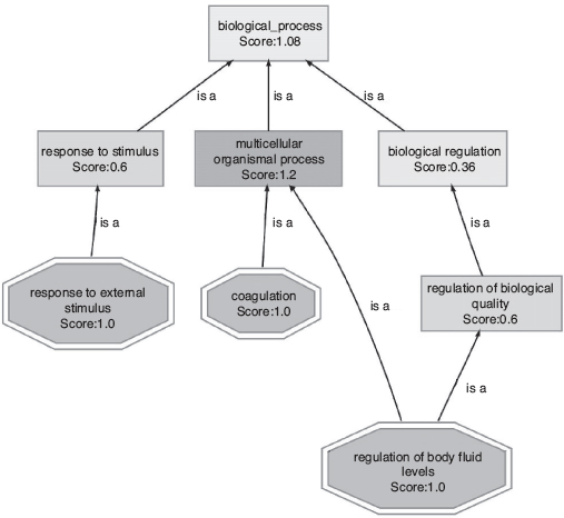
The complete set of gene ontology terms categorized into biological process, molecular function, and cellular component form a directed acyclic graph structure (DAG). We produce the DAG representation of the significant terms found the protein module in Figure 16.4. This representation depicts the relations between the significant terms at the hierarchical level. Going into the lower levels in such DAG representation signifies a function into more specific form. In this regard, we found the most specific significant biological process of this protein module to be the regulation of body fluid levels. Such specific findings are therefore very important in the perspective of systems biology.

16.8 CONCLUSIONS

This chapter includes an integrated approach of analyzing topological characteristics of PPINs. The approach used in this study for combining two topological properties can also be extended for combining multiple properties at a time. We use a heuristic mining algorithm to find out dense protein sets from the integrated interaction network. Here, the denseness of a subnetwork has been defined in a novel way by thresholding minimum association of each node with the others in the weighted subnetwork. The analytical studies provoke a new integrative approach of studying biological systems as initiated in [4].

The success of such topological studies highly depend on the accuracy and quality of the high-throughput interaction resources. Unfortunately, the enormous volume of interaction information accumulated by various research groups worldwide principally focus on positive interactions. Researchers are generally biased to finding protein pairs that physically or functionally interact, not those having no provable interactions. There is no doubt that casting aside the negative interaction data is a major drawback of interactome analysis. Recently, it has been empirically validated that negative training data sets can add potentials to the final outcome of computational analysis on biological data [37]. Analyzing PPINs covering both validated positive and negative interaction information will thus be a promising improvement in this direction.

ACKNOWLEDGMENT

S. Bandyopadhyay gratefully acknowledges the financial support from the grant No.- DST/SJF/ET-02/2006-07 under the Swarnajayanti Fellowship scheme of the Department of Science and Technology, Government of India.

REFERENCES

1. A. Finkelstein, J. Hetherington, L. Li, O. Margoninski, P. Saffrey, R. Seymour, and A. Warner (2004), Computational challenges of systems biology, IEEE Computer, 37(5):26–33.

2. G. T. Reeves and S. E. Fraser (2009), Biological systems from an engineer’s point of view, PLoS Biol., 7(1):e1000021.

3. C. J. Tomlin and J. D. Axelrod (2007), Biology by numbers: mathematical modelling in developmental biology, Nat. Rev. Genet., 8(5):331–340.

4. I. Ulitsky and R. Shamir (2007), Identification of functional modules using network topology and high-throughput data, BMC Systems Biol., 1:8.

5. M. Bhattacharyya and S. Bandyopadhyay (2009), Mining the largest quasi-clique in human protein interactome. Proceedings of the International Conference on Adaptive and Intelligent Systems, Klagenfurt, Austria.

6. D. Jiang and J. Pei (2009), Mining frequent cross-graph quasi-cliques, ACM Trans. Knowledge Dis. Data, 2(4):16.

7. J. Pei, D. Jiang, and A. Zhang (2005), On mining cross-graph quasi-cliques. In Proceedings of the 11th ACM SIGKDD International Conference on Knowledge Discovery and Data Mining, pp. 228–238, Chicago, IL.

8. M. Bhattacharyya and S. Bandyopadhyay (2009), Integration of co-expression networks for gene clustering. Proceedings of the 7th International Conference on Advances in Pattern Recognition, pp. 355–358, Kolkata, India.

9. H. N. Chua, W. Hugo, G. Liu, X. Li, L. Wong, and S. K. Ng (2009), A probabilistic graph-theoretic approach to integrate multiple predictions for the protein-protein subnetwork prediction challenge. Ann. NY Acad. Sci., 1158:224–233.

10. I. Lee, S. V. Date, A. T. Adai, and E. M. Marcotte (2004), A probabilistic functional network of yeast genes, Science, 306:1555–1558.

11. Q. A. Justman, Z. Serber, Jr. J. E. Ferrell, H. El-Samad, and K. M. Shokat (2009), Tuning the activation threshold of a kinase network by nested feedback loops, Science, 324(5926):509–512.

12. M. E. Cusick, N. Klitgord, M. Vidal, and D. E. Hill (2005), Interactome: gateway into systems biology, Human Mol. Genet., 14(Rev. Issue 2):R171–R181.

13. S. C. Gad (2005), Drug Discovery Handbook. John Wiley & Sons, Inc., NY.

14. A. Panchenko and T. Przytycka (Eds.) (2008), Protein–protein interactions and networks: Identification, computer analysis, and prediction, Computational Biology, Vol. 9. Springer, NY.

15. R. Sharan, I. Ulitsky, and R. Shamir (2007), Network-based prediction of protein function, Mol. Systems Biol., 3:88.

16. A. L. Barabási and R. Albert (1999), Emergence of scaling in random networks, Science, 286:509–512.

17. D. J. Watts and S. H. Strogatz (1998), Collective dynamics of ‘small-world’ networks, Nature (London), 393:440–442.

18. G. D. Bader and C. W. Hogue (2003), An automated method for finding molecular complexes in large protein interaction networks, BMC Bioinformatics, 4:2.

19. O. Tastan, Y. Qi, J. G. Carbonell, and J. Klein-Seetharaman (2009), Prediction of interactions between hiv-1 and human proteins by information integration. Proceedings of the Pacific Symposium on Biocomputing, pp. 516–527, Hawaii.

20. C. Brun, F. Chevenet, D. Martin, J. Wojcik, A. Guenoche, and B. Jacq (2003), Functional classification of proteins for the prediction of cellular function from a protein-protein interaction network, Genome Biol., 5(1):R6.

21. I. M. Bomze, M. Budinich, P. M. Pardalos, and M. Pelillo (1999), The maximum clique problem. D. Z. Du and P. M. Pardalos (Eds.), Handbook of Combinatorial Optimization: Supplementary Volume A, pp. 1–74. Kluwer Academic, Dordrecht, The Netherlands.

22. X. Liu, J. Li and L. Wang (2008), Quasi-bicliques: Complexity and binding pairs. Computing and Combinatorics, Vol. LNCS 5092, pp. 255–264, Springer, NY.

23. L. Royer, M. Reimann, B. Andreopoulos, and M. Schroeder (2008), Unraveling protein networks with power graph analysis, PLoS Comput. Biol., 4(7):e1000108.

24. C. C. Lin, H. F. Juan, J. T. Hsian, Y. C. Hwang, H. Mori, and H. C. Huang (2009), Essential core of protein-protein interaction network in Escherichia coli., J. Proteome Res., 8(4):1925–1931.

25. J. Abello, M. G. C. Resende, and S. Sudarsky (2002), Massive quasi-clique detection, Theoretical Informatics, Vol. LNCS 2286, pp. 598–612. Springer, NY.

26. D. Bu, Y. Zhao, L. Cai, H. Xue, X. Zhu, H. Lu, J. Zhang, S. Sun, L. Ling, N. Zhang, G. Li, and R. Chen (2003), Topological structure analysis of the protein-protein interaction network in budding yeast. Nucleic Acids Res., 31(9):2443–2450.

27. H. Liu, J. Liu, and L. Wang (2007), Searching quasi-bicliques in proteomic data. Proceedings of the International Conference on Computational Intelligence and Security Workshops, pp. 77–80, Washington, DC.

28. H. Liu, J. Liu, and L. Wang (2008), Searching maximum quasi-bicliques from protein-protein interaction network, J. Biomed. Sci. Eng., 1:200–203.

29. J. F. Rual, K. Venkatesan, T. Hao, T. Hirozane-Kishikawa, and A. Dricot (2005), Towards a proteome-scale map of the human protein-protein interaction network, Nature (London), 437:1173–1178.

30. M. Altaf-Ul-Amin, Y. Shinbo, K. Mihara, K. Kurokawa, and S. Kanaya (2006), Development and implementation of an algorithm for detection of protein complexes in large interaction networks, BMC Bioinformatics, 7:207.

31. X. Yan, M. R. Mehan, Y. Huang, M. S. Waterman, P. S. Yu, and X. J. Zhou (2007), A graph-based approach to systematically reconstruct human transcriptional regulatory modules, Bioinformatics, 23:i577–i586.

32. M. R. Garey and D. S. Johnson (1979), Computers and Intractability: A Guide to the Theory of NP-Completeness. Freeman & Co., NY.

33. S. Bandyopadhyay and M. Bhattacharyya (2008), Mining the largest dense n-vertexlet in a fuzzy scale-free graph. In Technical Report No. MIU/TR-03/08, Machine Intelligence Unit, Indian Statistical Institute, Kolkata, India.

34. T. S. K. Prasad et al. (2009), Human protein reference database—2009 update, Nucleic Acids Res. (Database issue), 37:D767–D772.

35. F. Al-Shahrour, R. Dïaz-Uriarte, and J. Dopazo (2004), FatiGO: a web tool for finding significant associations of gene ontology terms with groups of genes, Bioinformatics, 20:578–580.

36. J. Setubal and J. Meidanis (1999), Introduction to Computational Molecular Biology, PWS Publishing Company, Boston.

37. S. Bandyopadhyay and R. Mitra (2009), TargetMiner: MicroRNA target prediction with systematic identification of tissue specific negative examples, Bioinformatics, 25(20):2625–2631.