Chapter 9

Managing Transactions and Data Integrity

WHAT’S IN THIS CHAPTER?

• Understanding essentials of ACID transactions
• Applying transactional guarantee in distributed systems
• Understanding Brewer’s CAP Theorem
• Exploring transactional support in NoSQL products

The best way to understand transactions and data integrity in the world of NoSQL is to first review these same concepts in the context of the familiar RDBMS environment. Once the fundamental transactional notions and vocabulary are established and a couple of use cases are illustrated, it gets easier to conceive how the transactional concepts are challenged in large-scale distributed environments; places where NoSQL shines.

Not all NoSQL products share a similar view of transactions and data integrity. So once the broad and generalized expectations of transactional integrity in large-scale distributed systems is explained, it’s pertinent to show how it’s implemented in specific products and that is exactly how this chapter approaches the topic.

So to get started, you need to begin with ACID.

RDBMS AND ACID

ACID, which stands for Atomicity, Consistency, Isolation, and Durability, has become the gold standard to define the highest level of transactional integrity in database systems. As the acronym suggests it implies the following:

• Atomicity — Either a transactional operation fully succeeds or completely fails. Nothing that is inconsistent between the two states is acceptable. The canonical example that illustrates this property is transferring funds from one account, say A, to another, say B. If $100 needs to be transferred from A to B, $100 needs to be debited from (taken out of) A and credited to (deposited into) B. This could logically mean the operation involves two steps: debit from A and credit to B. Atomicity implies that if for some reason, debit from A occurs successfully and then the operation fails, the entire operation is rolled back and the operation is not left in an inconsistent state (where the money has been debited from A but not credited to B).
• Consistency — Consistency implies that data is never persisted if it violates a predefined constraint or rule. For example, if a particular field states that it should hold only integer values, then a float value is not accepted or is rounded to the nearest integer and then saved. Consistency is often confused with atomicity. Also, its implication in the context of RDBMS often relates to unique constraints, data type validations, and referential integrity. In a larger application scenario, consistency could include more complex rules imposed on the data but in such cases the task of maintaining consistency is mostly left to the application.
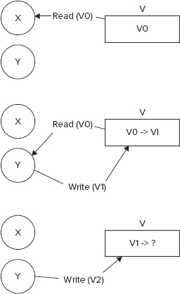
• Isolation — Isolation gets relevant where data is accessed concurrently. If two independent processes or threads manipulate the same data set, it’s possible that they could step on each other’s toes. Depending on the requirement, the two processes or threads could be isolated from each other. As an example, consider two processes, X and Y, modifying the value of a field V, which holds an initial value V0. Say X reads the value V0 and wants to update the value to V1 but before it completes the update Y reads the value V0 and updates it to V2. Now when X wants to write the value V1 it finds that the original value has been updated. In an uncontrolled situation, X would overwrite the new value that Y has written, which may not be desirable. Look at Figure 9-1 to view the stated use case pictorially. Isolation assures that such discrepancies are avoided. The different levels and strategies of isolation are explained later in a following section.

  FIGURE 9-1

  
• Durability — Durability implies that once a transactional operation is confirmed, it is assured. The case where durability is questioned is when a client program has received confirmation that a transactional operation has succeeded but then a system failure prevents the data from being persisted to the store. An RDBMS often maintains a transaction log. A transaction is confirmed only after it’s written to the transaction log. If a system fails between the confirmation and the data persistence, the transaction log is synchronized with the persistent store to bring it to a consistent state.

The ACID guarantee is well recognized and expected in RDBMSs. Often, application frameworks and languages that work with RDBMS attempt to extend the ACID promise to the entire application. This works fine in cases where the entire stack, that is, the database and the application, resides on a single server or node but it starts getting stretched the moment the stack constituents are distributed out to multiple nodes.

Isolation Levels and Isolation Strategies

A strict isolation level directly impacts concurrency. Therefore, to allow concurrent processing the isolation requirements are often relaxed. The ISO/ANSI SQL standard defines four isolation levels that provide varying and incremental levels of isolation. The four levels are as follows:

• Read Uncommitted
• Read Committed
• Repeatable Read
• Serializable

In addition, no isolation or complete chaos could be considered a fifth level of isolation. Isolation levels can be clearly explained using examples so I will resort to using one here as well. Consider a simple collection (or table in the RDBMS world) of data as shown in Table 9-1.

TABLE 9-1: Sample Data for Understanding Isolation Levels

Now, say two independent transactions, Transaction 1 and Transaction 2, manipulate this data set concurrently. The sequence is as follows:

Depending on the isolation level the result will be different. If the isolation level is set to Read Uncommitted, Transaction 1 sees the updated but uncommitted change by Transaction 2 (from step 2) in step 3. As in step 4, such uncommitted changes can be rolled back, and therefore, such reads are appropriately called dirty reads. If the isolation level is a bit stricter and set to the next level — Read Committed — Transaction 1 doesn’t see the uncommitted changes when it re-reads the data in step 3.

Now, consider interchanging steps 3 and 4 and a situation where Transaction 2 commits the update. The new sequence of steps is as follows:

The Read Uncommitted isolation level isn’t affected by the change in steps. It’s the level that allows dirty reads, so obviously committed updates are read without any trouble. Read Committed behaves differently though. Now, because changes have been committed in step 3, Transaction 1 reads the updated data in step 4. The reads from step 1 and step 4 are not the same so it’s a case of no-repeatable reads.

As the isolation level is upped to Repeatable Read, the reads in step 1 and step 4 are identical. That is, Transaction 1 is isolated from the committed updates from Transaction 2 while they are both concurrently in process. Although a repeatable read is guaranteed at this level, insertion and deletion of pertinent records could occur. This could lead to inclusion and exclusion of data items in subsequent reads and is often referred to as a phantom read. To walk through a case of phantom read consider a new sequence of steps as follows:

Now, with isolation set to the Repeatable Read level, the data set returned to Transaction 1 in step 1 and step 4 are not same. Step 4 sees the data item with id 4 in addition to the original three data points. To avoid phantom reads you need to involve range locks for reads and resort to using the highest level of isolation, Serializable. The term serializable connotes a sequential processing or serial ordering of transactions but that is not always the case. It does block other concurrent transactions when one of them is working on the data range, though. In some databases, snapshot isolation is used to achieve serializable isolation. Such databases provide a transaction with a snapshot when they start and allow commits only if nothing has changed since the snapshot.

Use of higher isolation levels enhances the possibility of starvation and deadlocks. Starvation occurs when one transaction locks out resources from others to use and deadlock occurs when two concurrent transactions wait on each other to finish and free up a resource.

With the concepts of ACID transactions and isolation levels reviewed, you are ready to start exploring how these ideas play out in highly distributed systems.

DISTRIBUTED ACID SYSTEMS

To understand fully whether or not ACID expectations apply to distributed systems you need to first explore the properties of distributed systems and see how they get impacted by the ACID promise.

Distributed systems come in varying shapes, sizes, and forms but they all have a few typical characteristics and are exposed to similar complications. As distributed systems get larger and more spread out, the complications get more challenging. Added to that, if the system needs to be highly available the challenges only get multiplied. To start out, consider an elementary situation as illustrated in Figure 9-2.

Even in this simple situation with two applications, each connected to a database and all four parts running on a separate machine, the challenges of providing the ACID guarantee is not trivial. In distributed systems, the ACID principles are applied using the concept laid down by the open XA consortium, which specifies the need for a transaction manager or coordinator to manage transactions distributed across multiple transactional resources. Even with a central coordinator, implementing isolation across multiple databases is extremely difficult. This is because different databases provide isolation guarantees differently. A few techniques like two-phase locking (and its variant Strong Strict Two-Phase Locking or SS2PL) and two-phase commit help ameliorate the situation a bit. However, these techniques lead to blocking operations and keep parts of the system from being available during the states when the transaction is in process and data moves from one consistent state to another. In long-running transactions, XA-based distributed transactions don’t work, as keeping resources blocked for a long time is not practical. Alternative strategies like compensating operations help implement transactional fidelity in long-running distributed transactions.

The challenges of resource unavailability in long-running transactions also appear in high-availability scenarios. The problem takes center stage especially when there is less tolerance for resource unavailability and outage.

A congruent and logical way of assessing the problems involved in assuring ACID-like guarantees in distributed systems is to understand how the following three factors get impacted in such systems:

• Consistency
• Availability
• Partition Tolerance

Consistency, Availability, and Partition Tolerance (CAP) are the three pillars of Brewer’s Theorem that underlies much of the recent generation of thinking around transactional integrity in large and scalable distributed systems. Succinctly put, Brewer’s Theorem states that in systems that are distributed or scaled out it’s impossible to achieve all three (Consistency, Availability, and Partition Tolerance) at the same time. You must make trade-offs and sacrifice at least one in favor of the other two. However, before the trade-offs are discussed, it’s important to explore some more on what these three factors mean and imply.

Consistency

Consistency is not a very well-defined term but in the context of CAP it alludes to atomicity and isolation. Consistency means consistent reads and writes so that concurrent operations see the same valid and consistent data state, which at minimum means no stale data.

In ACID, consistency means that data that does not satisfy predefined constraints is not persisted. That’s not the same as the consistency in CAP.

Brewer’s Theorem was conjectured by Eric Brewer and presented by him (www.cs.berkeley.edu/~brewer/cs262b-2004/PODC-keynote.pdf) as a keynote address at the ACM Symposium on the Principles of Distributed Computing (PODC) in 2000. Brewer’s ideas on CAP developed as a part of his work at UC Berkeley and at Inktomi. In 2002, Seth Gilbert and Nancy Lynch proved Brewer’s conjecture and hence it’s now referred to as Brewer’s Theorem (and sometimes as Brewer’s CAP Theorem). In Gilbert and Lynch’s proof, consistency is considered as atomicity. Gilbert and Lynch’s proof is available as a published paper titled “Brewer’s Conjecture and the Feasibility of Consistent, Available, Partition-Tolerant Web Services” and can be accessed online at http://theory.lcs.mit.edu/tds/papers/Gilbert/Brewer6.ps.

In a single-node situation, consistency can be achieved using the database ACID semantics but things get complicated as the system is scaled out and distributed.

Availability

Availability means the system is available to serve at the time when it’s needed. As a corollary, a system that is busy, uncommunicative, or unresponsive when accessed is not available. Some, especially those who try to refute the CAP Theorem and its importance, argue that a system with minor delays or minimal hold-up is still an available system. Nevertheless, in terms of CAP the definition is not ambiguous; if a system is not available to serve a request at the very moment it’s needed, it’s not available.

That said, many applications could compromise on availability and that is a possible trade-off choice they can make.

Partition Tolerance

Parallel processing and scaling out are proven methods and are being adopted as the model for scalability and higher performance as opposed to scaling up and building massive super computers. The past few years have shown that building giant monolithic computational contraptions is expensive and impractical in most cases. Adding a number of commodity hardware units in a cluster and making them work together is a more cost-, algorithm-, and resource-effective and efficient solution. The emergence of cloud computing is a testimony to this fact.

Read the note titled “Vertical Scaling Challenges and Fallacies of Distributed Computing” to understand some of trade-offs associated with the two alternative scaling strategies.

Because scaling out is the chosen path, partitioning and occasional faults in a cluster are a given. The third pillar of CAP rests on partition tolerance or fault-tolerance. In other words, partition tolerance measures the ability of a system to continue to service in the event a few of its cluster members become unavailable.

UPHOLDING CAP

Achieving consistency, availability, and partition tolerance at all times in a large distributed system is not possible and Brewer’s Theorem already states that. You can and should read Gilbert and Lynch’s proof to delve deeper into how and why Brewer is correct. However, for a quick and intuitive illustration, I explain the central ideas using a simple example, which is shown in a set of two figures: Figures 9-3 and 9-4.

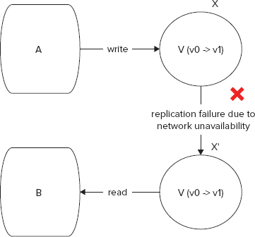
Figures 9-3 and 9-4 show two nodes of a clustered system where processes A and B access data from X and X’, respectively. X and X’ are replicated data stores (or structures) and hold copies of the same data set. A writes to X and B reads from X’. X and X’ synchronize between each other. V is an entity or object stored in X and X’. V has an original value v0. Figure 9-3 shows a success use case where A writes v1 to V (updating its value from v0), v1 gets synchronized over from X to X’, and then B reads v1 as the value of V from X’. Figure 9-4, on the other hand, shows a failure use case where A writes v1 to V and B reads the value of V, but the synchronizing between X and X’ fails and therefore the value read by B is not consistent with the most recent value of V. B still reads v0 whereas the latest updated value is v1.

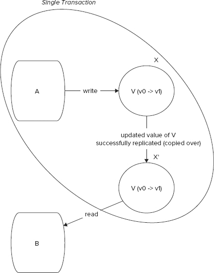
If you are to ensure that B always reads the correct value, you need to make sure that you synchronously copy the updated value v1 from X to X’. In other words, the two operations — (1) A updates the value of V in X from v0 to v1 and (2) The updated value of V (that is, v1) is copied over from X to X’ — would need to be in a single transaction. Such a setting is depicted in Figure 9-5. This setup would guarantee atomicity in this distributed transaction but would impact latency and availability. If a failure case as illustrated in Figure 9-4 arises, resources will be blocked until the network heals and the updated value replication between X and X’ is complete.

If the process of data replication between X and X’ is asynchronous, there is no way of knowing the exact time when it occurs. If one doesn’t know when an event exactly occurs there is obviously no way of guaranteeing if the event has occurred or not unless one seeks explicit consensus or confirmation. If you need to wait for a consensus or confirmation, the impact on latency and availability of the asynchronous operation is not very different from that of the synchronous operation. So one way or the other where systems are distributed and faults can occur, the trade-off among data consistency, system availability, and partition tolerance needs to be understood and choices need to be made where two of these are favored over the third, and therefore, the third is compromised.

The choices could be as follows:

• Option 1 — Availability is compromised but consistency and partition tolerance are preferred over it.
• Option 2 — The system has little or no partition tolerance. Consistency and availability are preferred.
• Option 3 — Consistency is compromised but systems are always available and can work when parts of it are partitioned.

Traditional transactional RDBMS chooses option 1 under circumstances of horizontal scaling. In such cases, the availability is affected by many factors, including the following:

• Delays due to network lag
• Communication bottlenecks
• Resource starvation
• Hardware failure leading to partitioning

Compromising on Availability

In extreme cases, when nodes fail the system may become completely unavailable until it’s healed and the system is restored to a consistent state. Although unavailability seems terribly detrimental to business continuity, sometimes that’s the only choice at hand. You can have either a consistent data state or the transaction fails. This is typical of money- and time-sensitive transactions where compensating transactions in failure cases is completely unacceptable or bears a very high cost. The quintessential example of money transfer between two accounts is often quoted as an example for such a use case. In real life, though, banks sometimes have relaxed alternatives for such extreme cases as well and you will learn about them a little later when I discuss weak consistency.

In many situations, systems — including those based on RDBMS — provide for backup and quick replication and recovery from failure. This means the system may still be unavailable but for a very short time. In a majority of cases, minor unavailability is not catastrophic and is a viable choice.

Compromising on Partition Tolerance

In some cases, it’s better not to accommodate partition tolerance. A little while back I stated that in horizontally scaled systems, node failure is a given and the chances of failure increase as the number of nodes increases. How then can partition intolerance be an option? Many people confuse partition tolerance with fault tolerance but the two are not one and the same. A system that does not service partitions that gets isolated from the network but allows for recovery by re-provisioning other nodes almost instantaneously is fault tolerant but not partition tolerant.

Google’s Bigtable is a good example of a data store that is highly available and provides for strong consistency but compromises on partition tolerance. The system is fault tolerant and easily survives a node failure but it’s not partition tolerant. More appropriately, under a fault condition it identifies primary and secondary parts of a partition and tries to resolve the problem by establishing a quorum.

To understand this a bit further, it may be worthwhile to review what you learned earlier about Bigtable (and its clones like HBase) in Chapter 4. Reading the section titled “HBase Distributed Storage Architecture” from Chapter 4 would be most pertinent.

Bigtable and its clones use a master-worker pattern where column-family data is stored together in a region server. Region servers are dynamically configured and managed by a master. In Google’s Bigtable, data is persisted to the underlying Google FileSystem (GFS) and the entire infrastructure is coordinated by Chubby, which uses a quorum algorithm like Paxos to assure consistency. In the case of HBase, Hadoop Distributed FileSystem (HDFS) carries out the same function as GFS and ZooKeeper replaces Chubby. ZooKeeper uses a quorum algorithm to recover from a failed node. On failure, ZooKeeper determines which is the primary partition and which one is the secondary. Based on these inferences, ZooKeeper directs all read and write operations to the primary partition and makes the secondary one a read-only partition until this problem is resolved.

In addition, Bigtable and HBase (and its underlying filesystems, GFS and HDFS, respectively) store three copies of every data set. This assures consistency by consensus when one out of the three copies fails or is out of synch. Having less than three copies does not assure consensus.

Compromising on Consistency

In some situations, availability cannot be compromised and the system is so distributed that partition tolerance is required. In such cases, it may be possible to compromise strong consistency. The counterpart of strong consistency is weak consistency, so all such cases where consistency is compromised could be clubbed in this bundle. Weak consistency, is a spectrum so this could include cases of no consistency and eventual consistency. Inconsistent data is probably not a choice for any serious system that allows any form of data updates but eventual consistency could be an option. Eventual consistency again isn’t a well-defined term but alludes to the fact that after an update all nodes in the cluster see the same state eventually. If the eventuality can be defined within certain limits, then the eventual consistency model could work.

For example, a shopping cart could allow orders even if it’s not able to confirm with the inventory system about availability. In a possible limit case, the product ordered may be out of stock. In such a case, the order could be taken as a back order and filled when the inventory is restocked. In another example, a bank could allow a customer to withdraw up to an overdraft amount even if it’s unable to confirm the available balance so that in the worst situation if the money isn’t sufficient the transaction could still be valid and the overdraft facility could be used.

To understand eventual consistency, one may try to illustrate a situation in terms of the following three criteria:

• R — Number of nodes that are read from.
• W — Number of nodes that are written to.
• N — Total number of nodes in the cluster.

Different combinations of these three parameters can have different impacts on overall consistency. Keeping R < N and W < N allows for higher availability. Following are some common situations worth reviewing:

• R + W > N — In such situations, a consistent state can easily be established, because there is an overlap between some read and write nodes. An extreme case when R = N and W = N (that is, R + W = 2N) the system is absolutely consistent and can provide an ACID guarantee.
• R = 1, W = N — When a system has more reads than writes, it makes sense to balance the read load out to all nodes of the cluster. When R = 1, each node acts independent of any other node as far as a read operation is concerned. A W = N write configuration means all nodes are written to for an update. In cases of a node failure the entire system then becomes unavailable for writes.
• R = N, W = 1 — When writing to one node is enough, the chance of data inconsistency can be quite high. However, in an R = N scenario, a read is only possible when all nodes in the cluster are available.
• R = W = ceiling ((N + 1)/2) — Such a situation provides an effective quorum to provide eventual consistency.

Eric Brewer and his followers coined the term BASE to denote the case of eventual consistency. BASE, which stands for Basically Available Soft-state Eventually consistent, is obviously contrived and was coined to counter ACID. However, ACID and BASE are not opposites but really depict different points in the consistency spectrum.

Eventual consistency can manifest in many forms and can be implemented in many different ways. A possible strategy could involve messaging-oriented systems and another could involve a quorum-based consensus. In a messaging-oriented system you could propagate an update using a message queue. In the simplest of cases, updates could be ordered using unique sequential ids. Chapter 4 explains some of the fundamentals of Amazon Dynamo and its eventual consistency model. You may want to review that part of the chapter.

In the following sections, I explain how consistency applies to a few different popular NoSQL products. This isn’t an exhaustive coverage but a select survey of a couple of them. The essentials of the consistency model in Google’s Bigtable and HBase has already been covered so I will skip those. In this section, consistency in a few others, namely document databases and eventually consistent flag bearers like Cassandra, will be explored.

CONSISTENCY IMPLEMENTATIONS IN A FEW NOSQL PRODUCTS

In this section, consistency in distributed document databases, namely MongoDB and CouchDB, is explained first.

Distributed Consistency in MongoDB

MongoDB does not prescribe a specific consistency model but defaults in favor of strong consistency. In some cases, MongoDB can be and is configured for eventual consistency.

In the default case of an auto-sharded replication-enabled cluster, there is a master in every shard. The consistency model of such a deployment is strong. In some other cases, though, you could deploy MongoDB for greater availability and partition tolerance. One such case could be one master, which is the node for all writes, and multiple slaves for read. In the event a slave is detached from the cluster but still servicing a client, it could potentially offer stale data. On partition healing the slave would receive all updates and provide for eventual consistency.

Eventual Consistency in CouchDB

CouchDB’s eventual consistency model relies on two important properties:

• Multiversion Concurrency Control (MVCC)
• Replication

Every document in CouchDB is versioned and all updates to a document are tagged with a unique revision number. CouchDB is a highly available and distributed system that relaxes consistency in favor of availability.

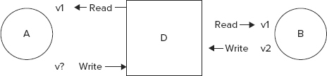
At the time of a read operation, a client (A) accesses a versioned document with a current revision number. For sake of specificity let’s assume the document is named D and its current version or revision number is v1. As client A is busy reading and possibly contemplating updating the document, client B accesses the same document D and also learns that its latest version is v1. B in an independent thread or process that manipulates D. Next, client B is ready to update the document before A returns. It updates D and increments its version or revision number to v2. When client A subsequently returns with an update to document D, it realizes that the document has been updated since the snapshot it accessed at the time of read.

This creates a conflicting situation at commit time. Luckily, version or revision numbers are available to possibly resolve the conflict. See Figure 9-6 for a pictorial representation of the conflicting update use case just illustrated.

Such conflicts can often be resolved by client A re-reading D before it’s ready for committing a new update. On re-read, if A discovers the snapshot version it’s working with (in this case v1) is stale, it can possibly re-apply the updates on the newest read and then commit the changes. Such methods of conflict resolution are commonly seen in version control software. Many current version control software products like Git and Mercurial have adopted MVCC to manage data fidelity and avoid commit conflicts.

CouchDB stores are scalable distributed databases so while MVCC resolves the conflict resolution scenarios in a single instance it doesn’t necessarily solve the issue of keeping all copies of the database current and up to date. This is where replication takes over. Replication is a common and well-established method for synchronizing any two data storage units. In its simplest form the file synchronization program rsync achieves the same for filesystem units like a folder or a directory.

Data in all nodes of a CouchDB cluster eventually becomes consistent with the help of the process of replication. The replication in CouchDB is both incremental and fault-tolerant. Therefore, only changes (or delta updates) are propagated at the time of replication and the process recovers gracefully if it fails, while the changes are being transmitted. CouchDB replication is state aware and on failure, it picks up where it stopped last. Therefore, redundant restarts are avoided and the inherent tendency of network failure or node unavailability is considered as a part of the design.

CouchDB’s eventual consistency model is both effective and efficient. CouchDB clusters are typically master-master nodes so each node can independently service requests and therefore enhance both availability and responsiveness.

Having surveyed the document databases, let’s move on to cover a few things about the eventual consistency model in Apache Cassandra.

Eventual Consistency in Apache Cassandra

Apache Cassandra aims to be like Google Bigtable and Amazon Dynamo. From a viewpoint of the CAP Theorem, this means Cassandra provisions for two trade-off choices:

• Favor consistency and availability — The Bigtable model, which you were exposed to earlier in this chapter.
• Favor availability and partition-tolerance — The Dynamo model, which you also learned about earlier in this chapter.

Cassandra achieves this by leaving the final consistency configuration in the hands of the developer. As a developer, your choices are as follows:

• Set R + W > N and achieve consistency, where R, W, and N being number of read replica nodes, number of write replicas, and total number of nodes, respectively.
• Achieve a Quorum by setting R = W = ceiling ((N+1)/2). This is the case of eventual consistency.

You can also set a write consistency all situation where W = N, but such a configuration can be tricky because failure can render the entire application unavailable.

Finally, I will quickly look at the consistency model in Membase.

Consistency in Membase

Membase is a Memcached protocol compatible distributed key/value store that provides for high availability and strong consistency but does not favor partition tolerance. Membase is immediately consistent. In cases of partitioning you could replicate Membase stores from master to slave replicas using an external tool but this isn’t a feature of the system.

Also, Membase, like Memcached, is adept at keeping a time-sensitive cache. In a strong and immediate consistency model, purging data beyond defined time intervals is easily and reliably supported. Supporting inconsistency windows for time-sensitive data can put forth its own challenges.

With the essentials of transaction management in NoSQL covered and a few products surveyed it may be appropriate to summarize and wrap the chapter up.

SUMMARY

Although succinct, this chapter is possibly one of the most important chapters in the book. This chapter clearly explained the notions of ACID and its possible alternative, BASE. It explained Brewer’s CAP Theorem and tried to relate its significance to distributed systems, which are increasingly becoming the norm in popular and widely used systems.

Consistency and its varying forms, strong and weak, were analyzed and eventual consistency was proposed as a viable alternative for higher availability under cases of partitioning.

Strong consistency advocates have often declined to consider NoSQL databases seriously due to its relaxed consistency configurations. Though consistency is an important requirement in many transactional systems, the strong-or-nothing approach has created a lot of fear, uncertainty, and doubt among users. Hopefully, this chapter laid out the choices explicitly for you to understand.

Last but not the least, although the chapter explained eventual consistency, it didn’t necessarily recommend it as a consistency model. Eventual consistency has its place and should be used where it safely provides high availability under partition conditions. However, you must bear in mind that eventual consistency is fraught with potential trouble. It’s neither trivial nor elementary to design and architect applications effortlessly to work under the eventual consistency model. If transactional integrity is important and the lack of it can severely disrupt normal operations, you should adopt eventual consistency only with extreme caution, fully realizing the pros and cons of your choice.