Chapter 3

Interfacing and Interacting with NoSQL

WHAT’S IN THIS CHAPTER?

• How to access the popular NoSQL databases
• Examples of data storage in the popular NoSQL stores
• How to query collections in popular NoSQL stores
• Introduction to drivers and language bindings for popular NoSQL databases

This chapter introduces the essential ways of interacting with NoSQL data stores. The types of NoSQL stores vary and so do the ways of accessing and interacting with them. The chapter attempts to summarize a few of the most prominent of these disparate ways of accessing and querying data in NoSQL databases. By no means is the coverage exhaustive, although it is fairly comprehensive to get you started on a strong footing.

NoSQL is an evolving technology and its current pace of change is substantial. Therefore, the ways of interacting with it are evolving as NoSQL stores are used in newer contexts and interfaced from newer programming languages and technology platforms. So be prepared for continued learning and look out for possible standardization in the future.

IF NO SQL, THEN WHAT?

A big reason for the popularity of relational databases is their standardized access and query mechanism using SQL. SQL, short for structured query language, is the language you speak when talking to relational databases. It involves a simple intuitive syntax and structure that users become fluent in within a short period of time. Based on relational algebra, SQL allows users to fetch records from a single collection or join records across tables. To reinforce its simplicity, here’s a walk through of a few simple examples:

• To fetch all data from a table that maintains the names and e-mail addresses of all the people in an organization, use SELECT * FROM people. The name of the table in this case is people.
• To get just a list of names of all the people from the people table, use SELECT name FROM people. The name is stored in a column called name.
• To get a subset from this list, say only those who have a Gmail account, use SELECT * FROM people where email LIKE '%gmail.com'.
• To get a list of people with a list of books they like, assuming that names of people and titles of books they like are in a separate but associated table named books_people_like, use SELECT people.name, books_people_like.book_title FROM people, books_people_like WHERE people.name = books_people_like.person_name. The table books_people_like has two columns: person_name and title, where person_name references the same set of values as the name column of the people table and title column stores book titles.

Although the benefits of SQL are many, it has several drawbacks as well. The drawbacks typically show up when you deal with large and spare data sets. However, in NoSQL stores there is no SQL, or more accurately there are no relational data sets. Therefore, the ways of accessing and querying data are different. In the next few sections, you learn how accessing and querying data in NoSQL databases is different from those same processes in SQL. You also learn about the similarities that exist between these processes.

I begin by exploring the essentials of storing and accessing data.

Storing and Accessing Data

In the previous chapter you had a first taste of NoSQL through a couple of elementary examples. In that chapter you indulged in some basic data storage and access using the document store MongoDB and the eventually consistent store Apache Cassandra. In this section I build on that first experience and present a more detailed view into the world of NoSQL data storage and access. To explain the different ways of data storage and access in NoSQL, I first classify them into the following types:

• Document store — MongoDB and CouchDB
• Key/value store (in-memory, persistent and even ordered) — Redis and BerkeleyDB
• Column-family-based store — HBase and Hypertable
• Eventually consistent key/value store — Apache Cassandra and Voldermot

This classification is not exhaustive. For example, it leaves out the entire set of object databases, graph databases, or XML data stores, which are excluded from this book altogether. The classification does not segregate non-relational databases into disjoint and mutually exclusive sets either. A few NoSQL stores have features that cut across the categories listed here. The classification merely sorts the non-relational stores into logical bundles by putting them within a set that best describes them.

As I discuss storage, access, and querying in NoSQL, I restrict the discussion to only a few of the categories listed and consider a small subset of the available products. I cover only the most popular ones. Learning to interface and interact with even a couple of NoSQL databases establishes a few fundamentals and common underpinning ideas in NoSQL. It will also prepare you for more advanced topics and more exhaustive coverage in the remaining chapters in this book.

Since you have been introduced to MongoDB, a document store, in the previous chapter, I will start the storage and access details with document databases.

To leverage the learn-by-example technique, I start here with a simple but interesting use case that illustrates the analysis of web server log data. The web server logs in the example follow the Combined Log Format for logging web server access and request activity. You can read more about the Apache web server Combined Log Format at http://httpd.apache.org/docs/2.2/logs.html#combined.

Storing Data In and Accessing Data from MongoDB

The Apache web server Combined Log Format captures the following request and response attributes for a web server:

• IP address of the client — This value could be the IP address of the proxy if the client requests the resource via a proxy.
• Identity of the client — Usually this is not a reliable piece of information and often is not recorded.
• User name as identified during authentication — This value is blank if no authentication is required to access the web resource.
• Time when the request was received — Includes date and time, along with timezone.
• The request itself — This can be further broken down into four different pieces: method used, resource, request parameters, and protocol.
• Status code — The HTTP status code.
• Size of the object returned — Size is bytes.
• Referrer — Typically, the URI or the URL that links to a web page or resource.
• User-agent — The client application, usually the program or device that accesses a web page or resource.

The log file itself is a text file that stores each request in a separate row. To get the data from the text file, you would need to parse it and extract the values. A simple elementary Python program to parse this log file can be quickly put together as illustrated in Listing 3-1.

LISTING 3-1: Log parser program

import re
import fileinput
lineRegex = re.compile(r'(d+.d+.d+.d+) ([^ ]*) ([^ ]*)
[([^]]*)] "([^"]*)" (d+) ([^ ]*) "([^"]*)" "([^"]*)"')

class ApacheLogRecord(object):

    def __init__(self, *rgroups ):
        self.ip, self.ident, 
        self.http_user, self.time, 
        self.request_line, self.http_response_code, 
        self.http_response_size, self.referrer, self.user_agent = rgroups
        self.http_method, self.url, self.http_vers = self.request_line.split()
    
    def __str__(self):
        return ' '.join([self.ip, self.ident, self.time, self.request_line,
        self.http_response_code, self.http_response_size, self.referrer,
        self.user_agent])

class ApacheLogFile(object):

    def __init__(self, *filename):
        self.f = fileinput.input(filename)

    def close(self):
        self.f.close()

    def __iter__(self):
        match = _lineRegex.match
        for line in self.f:
            m = match(line)
            if m:
                try:
                    log_line = ApacheLogRecord(*m.groups())
                    yield log_line
                except GeneratorExit:
                    pass
                except Exception as e:
                    print "NON_COMPLIANT_FORMAT: ", line, "Exception: ", e

apache_log_parser.py

After the data is available from the parser, you can persist the data in MongoDB. Because the example log parser is written in Python, it would be easiest to use PyMongo — the Python MongoDB driver — to write the data to MongoDB. However, before I get to the specifics of using PyMongo, I recommend a slight deviation to the essentials of data storage in MongoDB.

MongoDB is a document store that can persist arbitrary collections of data as long as it can be represented using a JSON-like object hierarchy. (If you aren’t familiar with JSON, read about the specification at www.json.org/. It’s a fast, lightweight, and popular data interchange format for web applications.) To present a flavor of the JSON format, a log file element extracted from the access log can be represented as follows:

{ 
    "ApacheLogRecord": {
        "ip": "127.0.0.1",
        "ident" : "-",
        "http_user" : "frank",
        "time" : "10/Oct/2000:13:55:36 -0700",
        "request_line" : {
            "http_method" : "GET",
            "url" : "/apache_pb.gif",
            "http_vers" : "HTTP/1.0",
        },
        "http_response_code" : "200",
        "http_response_size" : "2326",
        "referrer" : "http://www.example.com/start.html",
        "user_agent" : "Mozilla/4.08 [en] (Win98; I ;Nav)",
    },
}

The corresponding line in the log file is as follows:

127.0.0.1 - frank [10/Oct/2000:13:55:36 -0700] 
"GET /apache_pb.gif HTTP/1.0" 200 
2326 "http://www.example.com/start.html" "Mozilla/4.08 [en] 
(Win98; I ;Nav)"

MongoDB supports all JSON data types, namely, string, integer, boolean, double, null, array, and object. It also supports a few additional data types. These additional data types are date, object id, binary data, regular expression, and code. Mongo supports these additional data types because it supports BSON, a binary encoded serialization of JSON-like structures, and not just plain vanilla JSON. You can learn about the BSON specification at http://bsonspec.org/.

To insert the JSON-like document for the line in the log file into a collection named logdata, you could do the following in the Mongo shell:

doc = { 
    "ApacheLogRecord": {
        "ip": "127.0.0.1",
        "ident" : "-",
        "http_user" : "frank",
        "time" : "10/Oct/2000:13:55:36 -0700",
        "request_line" : {
            "http_method" : "GET",
            "url" : "/apache_pb.gif",
            "http_vers" : "HTTP/1.0",
        },
        "http_response_code" : "200",
        "http_response_size" : "2326",
        "referrer" : "http://www.example.com/start.html",
        "user_agent" : "Mozilla/4.08 [en] (Win98; I ;Nav)",
    },
};
db.logdata.insert(doc);

Mongo also provides a convenience method, named save, which updates a record if it exists in the collection and inserts it if it’s not.

In the Python example, you could save data in a dictionary (also referred to as map, hash map, or associative arrays in other languages) directly to MongoDB. This is because PyMongo — the driver — does the job of translating a dictionary to a BSON data format. To complete the example, create a utility function to publish all attributes of an object and their corresponding values as a dictionary like so:

def props(obj):
    pr = {}
    for name in dir(obj):
        value = getattr(obj, name)
        if not name.startswith('__') and not inspect.ismethod(value):
            pr[name] = value
    return pr

apache_log_parser_ mongodb.py

This function saves the request_line as a single element. You may prefer to save it as three separate fields: HTTP method, URL, and protocol version, as shown in Listing 3-1. You may also prefer to create a nested object hierarchy, which I touch upon a little later in this chapter during the discussion on queries.

With this function in place, storing data to MongoDB requires just a few lines of code:

    connection = Connection()
    db = connection.mydb
    collection = db.logdata
    alf = ApacheLogFile(<path to access_log>)
    for log_line in alf:
        collection.insert(props(log_line))
    alf.close()

apache_log_parser_mongodb.py

Isn’t that simple? Now that you have the log data stored, you can filter and analyze it.

Querying MongoDB

I used a current snapshot of my web server access log to populate a sample data set. If you don’t have access to web server logs, download the file named sample_access_log from the code download bundle available with this book.

After you have some data persisted in a Mongo instance, you are ready to query and filter that set. In the previous chapter you learned some essential querying mechanisms using MongoDB. Let’s revise some of those and explore a few additional concepts that relate to queries.

All my log data is stored in a collection named logdata. To list all the records in the logdata collection, fire up the Mongo shell (a JavaScript shell, which can be invoked with the help of the bin/mongo command) and query like so:

> var cursor = db.logdata.find()
> while (cursor.hasNext()) printjson(cursor.next());

This prints the data set in a nice presentable format like this:

{
    "_id" : ObjectId("4cb164b75a91870732000000"),
    "http_vers" : "HTTP/1.1",
    "ident" : "-",
    "http_response_code" : "200",
    "referrer" : "-",
    "url" : "/hi/tag/2009/",
    "ip" : "123.125.66.32",
    "time" : "09/Oct/2010:07:30:01 -0600",
    "http_response_size" : "13308",
    "http_method" : "GET",
    "user_agent" : "Baiduspider+(+http://www.baidu.com/search/spider.htm)",
    "http_user" : "-",
    "request_line" : "GET /hi/tag/2009/ HTTP/1.1"
}
{
    "_id" : ObjectId("4cb164b75a91870732000001"),
    "http_vers" : "HTTP/1.0",
    "ident" : "-",
    "http_response_code" : "200",
    "referrer" : "-",
    "url" : "/favicon.ico",
    "ip" : "89.132.89.62",
    "time" : "09/Oct/2010:07:30:07 -0600",
    "http_response_size" : "1136",
    "http_method" : "GET",
    "user_agent" : "Safari/6531.9 CFNetwork/454.4 Darwin/10.0.0 (i386) 
(MacBook5%2C1)",
    "http_user" : "-",
    "request_line" : "GET /favicon.ico HTTP/1.0"
}
...

Let’s dice through the query and the result set to explore a few more details of the query and response elements.

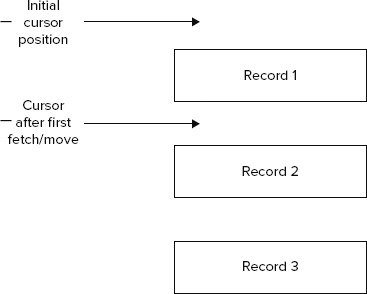
First, a cursor is declared and then all the data available in the logdata collection is fetched and assigned to it. Cursors or iterators are as common in relational databases as they are in MongoDB.

Look at Figure 3-1 to see how cursors work. The method db.logdata.find() returns all the records in the logdata collection, so you have the entire set to iterate over using the cursor. The previous code sample simply iterates through the elements of the cursor and prints them out. The printjson function prints out the elements in a nice JSON-style formatting for easy readability.

FIGURE 3-1

Although it’s nice to get hold of the entire collection, oftentimes all you need is a subset of available data. Next, you see how you can filter the collection and get a smaller set to work with. In the world of SQL it’s common to do the following two types of manipulations to get a subset of records:

• Restrict the output to only a select few columns instead of all the columns in a table.
• Restrict the number of rows in the table by filtering them on the basis of one or more column values.

In MongoDB, restricting the output to a few columns or attributes is not a smart strategy because each document is always returned in its entirety with all its attributes when fetched. Even then, you could choose to fetch only a few attributes for a document, although it would require you to restrict the collection. Restricting the document set to a subset of the entire collection is analogous to restricting SQL result sets to a limited set of rows. Remember the SQL WHERE clause!

I will fall back on my log file data example to illustrate ways to return a subset from a collection.

To get all log file records where http_response_code is 200, you can query like this:

db.logdata.find({ "http_response_code": "200" });

This query takes a query document, { "http_response_code": "200" }, defining the pattern, as an argument to the find method.

To get all log file records where http_response_code is 200 and http_vers (protocol version) is HTTP/1.1, you can query as follows:

db.logdata.find({ "http_response_code":"200", "http_vers":"HTTP/1.1" })

A query document is passed as an argument to the find method again. However, the pattern now includes two attributes instead of one.

To get all log file records where the user_agent was a Baidu search engine spider, you can query like so:

db.logdata.find({ "user_agent": /baidu/i })

If you look at the syntax carefully, you will notice that the query document actually contains a regular expression and not an exact value. The expression /baidu/i matches any document that has baidu in the user_agent value. The i flag suggests ignoring case, so all phrases whether baidu, Baidu, baiDU, or BAIDU would be matched. To get all log file records where user_agent starts with Mozilla, you can query as shown:

db.logdata.find({ "user_agent": /^Mozilla/ })

The possibility of using a regular expression for a query document pattern allows for innumerable possibilities and puts a lot of power in the hands of the user. However, as the cliché goes: with power comes responsibility. Therefore, use regular expressions to get the required subset but be aware that complex regular expressions could lead to expensive and complete scans, which for large data sets could be big trouble.

For fields that hold numeric values, comparison operators like greater than, greater than or equal to, less than, and less than or equal to also work. To get all log file records where response size is greater than 1111 k, you could query like so:

db.logdata.find({ "http_response_size" : { $gt : 1111 }})

Now that you have seen a few examples of restricting results to a subset, let’s cut down the number of fields to just one attribute or field: url. You can query the logdata collection to get a list of all URLs accessed by the MSN bot as shown:

db.logdata.find({ "user_agent":/msn/i }, { "url":true })

In addition, you could simply choose to restrict the number of rows returned in the last query to 10 as follows:

db.logdata.find({ "user_agent":/msn/i }, { "url":true }).limit(10)

Sometimes, all you need to know is the number of matches and not the entire documents. To find out the number of request from the MSN bot, you query the logdata collection like this:

db.logdata.find({ "user_agent":/msn/i }).count()

Although a lot more can be explained about the intricacies of advanced queries in MongoDB, I will leave that discussion for chapter 6, which covers advanced queries. Next, let’s turn to an alternate NoSQL store, Redis, to hold some data for us.

Storing Data In and Accessing Data from Redis

Redis is a persistent key/value store. For efficiency it holds the database in memory and writes to disks in an asynchronous thread. The values it holds can be strings, lists, hashes, sets, and sorted sets. It provides a rich set of commands to manipulate its collections and insert and fetch data.

If you haven’t already, install and set up Redis. Refer to Appendix A for help setting up Redis.

To explain Redis, I rely on the Redis command-line client (redis-cli) — and a simple use case that involves a categorized list of books.

To begin, start redis-cli and make sure it’s working. First, go to the Redis distribution folder. Redis is distributed as source. You can extract it anywhere in the file system and compile the source. Once compiled executables are available in the distribution folder. On some operating systems, symbolic links to executables are created at locations, where executables are commonly found. On my system Redis is available within a folder named Redis-2.2.2, which corresponds to the latest release of Redis. Start the Redis server by using the redis-server command. To use the default configuration, run ./redis-server from within the Redis distribution folder. Now run redis-cli to connect to this server. By default, the Redis server listens for connections on port 6379.

To save a key/value pair — { akey: "avalue" } — simply type the following, from within the Redis distribution folder:

./redis-cli set akey "avalue"

If you see OK on the console in response to the command you just typed, then things look good. If not, go through the installation instructions and verify that the setup is correct. To confirm that avalue is stored for akey, simply get the value for akey like so:

./redis-cli get akey

You should see a value in response to this request.

If you install Redis using "make install" after compiling from source, the redis-server and redis-cli will be added to /usr/local/bin by default. If /usr/local/bin is added to the PATH environment variable you will be able to run redis-server and redis-cli from any directory.

Redis supports a few different data structures, namely:

• Lists, or more specifically, linked lists — Collections that maintain an indexed list of elements in a particular order. With linked lists, access to either of the end points is fast irrespective of the number of elements in the list.
• Sets — Collections that store unique elements and are unordered.
• Sorted sets — Collections that store sorted sets of elements.
• Hashes — Collections that store key/value pairs.
• Strings — Collections of characters.

For the example at hand, I chose to use a set, because order isn’t important. I call my set books. Each book, which is a member of the set of books, has the following properties:

• Id
• Title
• Author
• Tags (a collection)

Each tag is identified with the help of the following properties:

• Id
• Name

Assuming the redis-server is running, open a redis-cli instance and input the following commands to create the first members of the set of books:

$ ./redis-cli incr next.books.id
(integer) 1
$ ./redis-cli sadd books:1:title "The Omnivore's Dilemma"
(integer) 1
$ ./redis-cli sadd books:1:author "Michael Pollan"

books_and_tags.txt

Redis offers a number of very useful commands, which are catalogued and defined at http://redis.io/commands. The first command in the previous code example generates a sequence number by incrementing the set member identifier to the next id. Because you have just started creating the set, the output of the increment is logically “1”. The next two commands create a member of the set named books. The member is identified with the id value of 1, which was just generated. So far, the member itself has two properties — title and author — the values for which are strings. The sadd command adds a member to a set. Analogous functions exist for lists, hashes and sorted sets. The lpush and rpush commands for a list add an element to the head and the tail, respectively. The zadd command adds a member to a sorted set.

Next, add a bunch of tags to the member you added to the set named books. Here is how you do it:

$ ./redis-cli sadd books:1:tags 1
(integer) 1
$ ./redis-cli sadd books:1:tags 2
(integer) 1
$ ./redis-cli sadd books:1:tags 3
(integer) 1
$ ./redis-cli sadd books:1:tags 4
(integer) 1
$ ./redis-cli sadd books:1:tags 5
(integer) 1
$ ./redis-cli sadd books:1:tags 6
(integer) 1

books_and_tags.txt

A bunch of numeric tag identifiers have been added to the member identified by the id value of 1. The tags themselves have not been defined any more than having been assigned an id so far. It may be worthwhile to break down the constituents of books:1:tags a bit further and explain how the key naming systems work in Redis. Any string, except those containing whitespace and special characters, are good choices for a key in Redis. Avoid very long or short keys. Keys can be structured in a manner where a hierarchical relationship can be established and nesting of objects and their properties can be established. It is a suggested practice and convention to use a scheme like object-type:id:field for key names. Therefore, a key such as books:1:tags implies a tag collection for a member identified by the id 1 within a set named “books.” Similarly, books:1:title means title field of a member, identified by an id value of 1, within the set of books.

After adding a bunch of tags to the first member of the set of books, you can define the tags themselves like so:

$ ./redis-cli sadd tag:1:name "organic"
(integer) 1
$ ./redis-cli sadd tag:2:name "industrialization"
(integer) 1
$ ./redis-cli sadd tag:3:name "local"
(integer) 1
$ ./redis-cli sadd tag:4:name "written by a journalist"
(integer) 1
$ ./redis-cli sadd tag:5:name "best seller"
(integer) 1
$ ./redis-cli sadd tag:6:name "insight"
(integer) 1

books_and_tags.txt

With tags defined, you establish the reciprocal relationship to associate books that have the particular tags. The first member has all six tags so you add it to each of the tags as follows:

$ ./redis-cli sadd tag:1:books 1
(integer) 1
$ ./redis-cli sadd tag:2:books 1
(integer) 1
$ ./redis-cli sadd tag:3:books 1
(integer) 1
$ ./redis-cli sadd tag:4:books 1
(integer) 1
$ ./redis-cli sadd tag:5:books 1
(integer) 1
$ ./redis-cli sadd tag:6:books 1
(integer) 1

books_and_tags.txt

After the cross-relationships are established, you would create a second member of the set like so:

$ ./redis-cli incr next.books.id
(integer) 2
$ ./redis-cli sadd books:2:title "Outliers"
(integer) 1
$ ./redis-cli sadd books:2:author "Malcolm Gladwell"
(integer) 1

books_and_tags.txt

The incr function is used to generate the id for the second member of the set. Functions like incrby, which allows increment by a defined step; decr, which allows you to decrement; and decrby, which allows you to decrement by a defined step, are also available as useful utility functions whenever sequence number generation is required. You can choose the appropriate function and define the step as required. For now incr does the job.

Next, you add the tags for the second member and establish the reverse relationships to the tags themselves as follows:

$ ./redis-cli sadd books:2:tags 6
(integer) 1
$ ./redis-cli sadd books:2:tags 5
(integer) 1
$ ./redis-cli sadd books:2:tags 4
(integer) 1
$ ./redis-cli sadd tag:4:books 2
(integer) 1
$ ./redis-cli sadd tag:5:books 2
(integer) 1
$ ./redis-cli sadd tag:6:books 2
(integer) 1

books_and_tags.txt

That creates the rudimentary but useful enough set of the two members. Next, you look at how to query this set.

Querying Redis

Continuing with the redis-cli session, you can first list the title and author of member 1, identified by the id 1, of the set of books as follows:

$ ./redis-cli smembers books:1:title
1. "The Omnivorexe2x80x99s Dilemma"
$ ./redis-cli smembers books:1:author
1. "Michael Pollan"

books_and_tags.txt

The special characters in the title string represent the apostrophe that was introduced in the string value.

You can list all the tags for this book like so:

$ ./redis-cli smembers books:1:tags
1. "4"
2. "1"
3. "2"
4. "3"
5. "5"
6. "6"

books_and_tags.txt

Notice that the list of tag ids is not ordered in the same way as they were entered. This is because sets have no sense of order within their members. If you need an ordered set, use a sorted set instead of a set.

Similarly, you can list title, author, and tags of the second book, identified by the id 2, like so:

$ ./redis-cli smembers books:2:title
1. "Outliers"
$ ./redis-cli smembers books:2:author
1. "Malcolm Gladwell"
$ ./redis-cli smembers books:2:tags
1. "4"
2. "5"
3. "6"

books_and_tags.txt

Now, viewing the set from the tags standpoint you can list all books that have the tag, identified by id 1 as follows:

$ ./redis-cli smembers tag:1:books
"1"

Tag 1 was identified by the name organic and you can query that like so:

$ ./redis-cli smembers tag:1:name
"organic"

Some tags like tag 6, identified by the name insight, have been attached to both the books in the set. You can confirm that by querying the set of books that have tag 6 like so:

$ ./redis-cli smembers tag:6:books
1. "1"
2. "2"

Next, you can list the books that have both tags 1 and 6, like so:

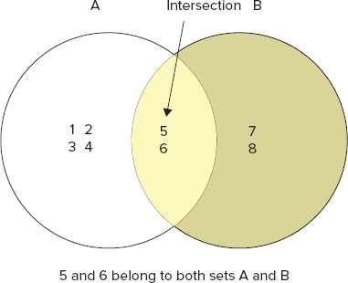
$ ./redis-cli sinter tag:1:books tag:6:books
"1"

The sinter command allows you to query for the intersection of two or more sets. If the word “intersection” has befuddled you, then review the Venn diagram in Figure 3-2 to set things back to normal.

FIGURE 3-2

You know both books 1 and 2 have tags 5 and 6, so a sinter between the books of tags 5 and 6 should list both books. You can run the sinter command to confirm this. The command and output are as follows:

$ ./redis-cli sinter tag:5:books tag:6:books
1. "1"
2. "2"

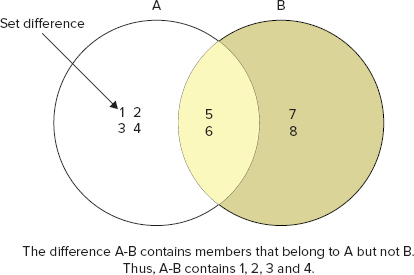
Like set intersection, you can also query for set union and difference. Figures 3-3 and 3-4 demonstrate what set union and difference imply.

FIGURE 3-3

FIGURE 3-4

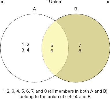
To create a union of all members that contain tags 1 and 6, you can use the following command:

$ ./redis-cli sunion tag:1:books tag:6:books
1. "1"
2. "2"

Both books 1 and 2 contain tags 5 and 6, so a difference set operation between books which have tag 5 and those that have tag 6 should be an empty set. Let’s see if it’s the case

$ ./redis-cli sdiff tag:5:books tag:6:books
(empty list or set)

Aren’t all these commands useful for some quick queries? As mentioned earlier, Redis has a rich set of commands for string values, lists, hashes, and sorted sets as well. However, I will skip those details for now and move on to another NoSQL store. Details of each of these Redis commands are covered in context later in this book.

Storing Data In and Accessing Data from HBase

HBase could very well be considered the NoSQL flag bearer. It’s an open-source implementation of the Google Bigtable, which you can read more about at http://labs.google.com/papers/bigtable.html. While key/value stores and non-relational alternatives like object databases have existed for a while, HBase and its associated Hadoop tools were the first piece of software to bring the relevance of large-scale Google-type NoSQL success catalysts in the hands of the masses.

HBase is not the only Google Bigtable clone. Hypertable is another one. HBase is also not the ideal tabular data store for all situations. There are eventually consistent data stores like Apache Cassandra and more that have additional features beyond those HBase provides. Before exploring where HBase is relevant and where it’s not, let’s first get familiar with the essentials of data store and querying in HBase. The relevance of HBase and other tabular databases is discussed later in this book.

As with the earlier two NoSQL data stores, I explain the HBase fundamentals with the help of an example and leave the more detailed architectural discussion for Chapter 4. The focus here is on data storage and access. For this section, I cook up a hypothetical example of a feed of blog posts, where you can extract and save the following pieces of information:

• Blog post title
• Blog post author
• Blog post content or body
• Blog post header multimedia (for example, an image)
• Blog post body multimedia (for example, an image, a video, or an audio file)

To store this data, I intend to create a collection named blogposts and save pieces of information into two categories, post and multimedia. So, a possible entry, in JSON-like format, could be as follows:

{
    "post" : {
        "title": "an interesting blog post",
        "author": "a blogger",
        "body": "interesting content",
    },
    "multimedia": {
        "header": header.png,
        "body": body.mpeg,
    },
}

blogposts.txt

or could be like so:

{
    "post" : {
        "title": "yet an interesting blog post",
        "author": "another blogger",
        "body": "interesting content",
    },
    "multimedia": {
        "body-image": body_image.png,
        "body-video": body_video.mpeg,
    },
}

blogposts.txt

Now if you look at the two sample data sets carefully you will notice that they both share the post and multimedia categories, but don’t necessarily have the same set of fields. Stated another way, their columns differ. In HBase jargon it means they have the same column-families — post and multimedia — but don’t have the same set of columns. Effectively, there are four columns within the multimedia column-family, namely, header, body, body-image, and body-video, and in some data points these columns have no value (null). In a traditional relational database you would have to create all four columns and set a few values to null as required. In HBase and column databases the data is stored by column and it doesn’t need to store values when they are null. Thus, these are great for sparse data sets.

To create this data set and save two data points, first start an HBase instance and connect to it using the HBase shell. HBase runs in a distributed environment where it uses a special filesystem abstraction to save data across multiple machines. In this simple case, though, I run HBase in a standalone and single-instance environment. If you have downloaded and extracted the latest HBase release distribution, start the default single-instance server by running bin/start-hbase.sh.

After the server is up and running, connect to the HBase local server by starting the shell like so:

bin/hbase shell

When connected, create the HBase collection blogposts with its two column-families, post and multimedia, as follows:

$ bin/hbase shell
HBase Shell; enter 'help<RETURN>' for list of supported commands.
Type "exit<RETURN>" to leave the HBase Shell
Version 0.90.1, r1070708, Mon Feb 14 16:56:17 PST 2011

hbase(main):001:0> create 'blogposts', 'post', 'multimedia'
0 row(s) in 1.7880 seconds

Populate the two data points like so:

hbase(main):001:0> put 'blogposts', 'post1', 'post:title',    
hbase(main):002:0* 'an interesting blog post'
0 row(s) in 0.5570 seconds

hbase(main):003:0> put 'blogposts', 'post1', 'post:author', 'a blogger'
0 row(s) in 0.0400 seconds

hbase(main):004:0> put 'blogposts', 'post1', 'post:body', 'interesting content'
0 row(s) in 0.0240 seconds

hbase(main):005:0> put 'blogposts', 'post1', 'multimedia:header', 'header.png'
0 row(s) in 0.0250 seconds

hbase(main):006:0> put 'blogposts', 'post1', 'multimedia:body', 'body.png'
0 row(s) in 0.0310 seconds

hbase(main):012:0> put 'blogposts', 'post2', 'post:title',
hbase(main):013:0* 'yet an interesting blog post'       
0 row(s) in 0.0320 seconds

hbase(main):014:0> put 'blogposts', 'post2', 'post:title',
hbase(main):015:0* 'yet another blog post'
0 row(s) in 0.0350 seconds

hbase(main):016:0> put 'blogposts', 'post2', 'post:author', 'another blogger'
0 row(s) in 0.0250 seconds

hbase(main):017:0> put 'blogposts', 'post2', 'post:author', 'another blogger'
0 row(s) in 0.0290 seconds

hbase(main):018:0> put 'blogposts', 'post2', 'post:author', 'another blogger'
0 row(s) in 0.0400 seconds

hbase(main):019:0> put 'blogposts', 'post2', 'multimedia:body-image',       
hbase(main):020:0* 'body_image.png'
0 row(s) in 0.0440 seconds

hbase(main):021:0> put 'blogposts', 'post2', 'post:body', 'interesting content'
0 row(s) in 0.0300 seconds

hbase(main):022:0> put 'blogposts', 'post2', 'multimedia:body-video',
hbase(main):023:0* 'body_video.mpeg'
0 row(s) in 0.0380 seconds

The two sample data points are given ids of post1 and post2, respectively. If you notice, I made a mistake while entering the title for post2 so I reentered it. I also reentered the same author information three items for post2. In the relational world, this would imply a data update. In HBase, though, records are immutable. Reentering data leads to creation of a newer version of the data set. This has two benefits: the atomicity conflicts for data update are avoided and an implicit built-in versioning system is available in the data store.

Now that the data is stored, you are ready to write a couple of elementary queries to retrieve it.

Querying HBase

The simplest way to query an HBase store is via its shell. If you are logged in to the shell already — meaning you have started it using bin/hbase shell and connected to the same local store where you just entered some data — you may be ready to query for that data.

To get all data pertaining to post1, simply query like so:

hbase(main):024:0> get 'blogposts', 'post1'
COLUMN                                             CELL
multimedia:body                                   timestamp=1302059666802,
value=body.png
multimedia:header                                 timestamp=1302059638880,
value=header.png
post:author                                       timestamp=1302059570361,
value=a blogger
post:body                                         timestamp=1302059604738,
value=interesting content
post:title                                        timestamp=1302059434638,
value=an interesting blog post
5 row(s) in 0.1080 seconds

blogposts.txt

This shows all the post1 attributes and their values. To get all data pertaining to post2, simply query like so:

hbase(main):025:0> get 'blogposts', 'post2'
COLUMN                                             CELL
multimedia:body-image                             timestamp=1302059995926,
value=body_image.png                                     
multimedia:body-video                             timestamp=1302060050405,
value=body_video.mpeg
post:author                                       timestamp=1302059954733,
value=another blogger                                            
post:body                                         timestamp=1302060008837,
value=interesting content                                              
post:title                                        timestamp=1302059851203,
value=yet another blog post
5 row(s) in 0.0760 seconds

blogposts.txt

To get a filtered list containing only the title column for post1, query like so:

hbase(main):026:0> get 'blogposts', 'post1', { COLUMN=>'post:title' }
COLUMN                                             CELL
post:title                                        timestamp=1302059434638,
value=an interesting blog post
1 row(s) in 0.0480 seconds

blogposts.txt

You may recall I reentered data for the post2 title, so you could query for both versions like so:

hbase(main):027:0> get 'blogposts', 'post2', { COLUMN=>'post:title', VERSIONS=>2 }
COLUMN                                             CELL
post:title                                        timestamp=1302059851203,
value=yet another blog post
post:title                                        timestamp=1302059819904,
value=yet an interesting blog post
2 row(s) in 0.0440 seconds

blogposts.txt

By default, HBase returns only the latest version but you can always ask for multiple versions or get an explicit older version if you like.

With these simple queries working, let’s move on to the last example data store, Apache Cassandra.

Storing Data In and Accessing Data from Apache Cassandra

In this section, I reuse the blogposts example from the previous section to show some of the fundamental features of Apache Cassandra. In the preceding chapter, you had a first feel of Apache Cassandra; now you will build on that and get familiar with more of its features.

To get started, go to the Apache Cassandra installation folder and start the server in the foreground by running the following command:

bin/cassandra -f

When the server starts up, run the cassandra-cli or command-line client like so:

bin/cassandra-cli -host localhost -port 9160

Now query for available keyspaces like so:

show keyspaces;

You will see the system and any additional keyspaces that you may have created. In the previous chapter, you created a sample keyspace called CarDataStore. For this example, create a new keyspace called BlogPosts with the help of the following script:

/*schema-blogposts.txt*/

create keyspace BlogPosts
    with replication_factor = 1
    and placement_strategy = 'org.apache.cassandra.locator.SimpleStrategy';

use BlogPosts;

create column family post
    with comparator = UTF8Type
    and read_repair_chance = 0.1
    and keys_cached = 100
    and gc_grace = 0
    and min_compaction_threshold = 5
    and max_compaction_threshold = 31;

create column family multimedia
    with comparator = UTF8Type
    and read_repair_chance = 0.1
    and keys_cached = 100
    and gc_grace = 0
    and min_compaction_threshold = 5
    and max_compaction_threshold = 31;

schema-blogposts.txt

Next, add the blog post sample data points like so:

Cassandra> use BlogPosts;
Authenticated to keyspace: BlogPosts
cassandra> set post['post1']['title'] = 'an interesting blog post';
Value inserted.
cassandra> set post['post1']['author'] = 'a blogger';
Value inserted.
cassandra> set post['post1']['body'] = 'interesting content';
Value inserted.
cassandra> set multimedia['post1']['header'] = 'header.png';
Value inserted.
cassandra> set multimedia['post1']['body'] = 'body.mpeg';
Value inserted.
cassandra> set post['post2']['title'] = 'yet an interesting blog post';
Value inserted.
cassandra> set post['post2']['author'] = 'another blogger';
Value inserted.
cassandra> set post['post2']['body'] = 'interesting content';
Value inserted.
cassandra> set multimedia['post2']['body-image'] = 'body_image.png';
Value inserted.
cassandra> set multimedia['post2']['body-video'] = 'body_video.mpeg';
Value inserted.

cassandra_blogposts.txt

That’s about it. The example is ready. Next you query the BlogPosts keyspace for data.

Querying Apache Cassandra

Assuming you are still logged in to the cassandra-cli session and the BlogPosts keyspace is in use, you can query for Post1 data like so:

get post['post1'];
=> (column=author, value=6120626c6f67676572, timestamp=1302061955309000)
=> (column=body, value=696e746572657374696e6720636f6e74656e74,
    timestamp=1302062452072000)
=> (column=title, value=616e20696e746572657374696e6720626c6f6720706f7374,
    timestamp=1302061834881000)
Returned 3 results.

cassandra_blogposts.txt

You could also query for a specific column like body-video for a post, say post2, within the multimedia column-family. The query and output would be as follows:

get multimedia['post2']['body-video'];
=> (column=body-video, value=626f64795f766964656f2e6d706567,
    timestamp=1302062623668000)

cassandra_blogposts.txt

LANGUAGE BINDINGS FOR NOSQL DATA STORES

Although the command-line client is a convenient way to access and query a NoSQL data store quickly, you probably want a programming language interface to work with NoSQL in a real application. As the types and flavors of NoSQL data stores vary, so do the types of programming interfaces and drivers. In general, though, there exists enough support for accessing NoSQL stores from popular high-level programming languages like Python, Ruby, Java, and PHP. In this section you look at the wonderful code generator Thrift and a few select language-specific drivers and libraries. Again, the intent is not to provide exhaustive coverage but more to establish the fundamental ways of interfacing NoSQL from your favorite programming language.

Being Agnostic with Thrift

Apache Thrift is an open-source cross-language services development framework. It’s a code-generator engine to create services to interface with a variety of different programming languages. Thrift originated in Facebook and was open sourced thereafter.

Thrift itself is written in C. To build, install, use, and run Thrift follow these steps:

This gets things ready. Next, run the Thrift server and then use a Thrift client to connect to the server.

You may not need to generate Thrift clients for a NoSQL store like Apache Cassandra that supports Thrift bindings but may be able to use a language-specific client instead. The language-specific client in turn leverages Thrift. The next few sections explore language bindings for a few specific data stores.

Language Bindings for Java

Java is a ubiquitous programming language. It may have lost some of its glory but it certainly hasn’t lost its popularity or pervasiveness. In this section I explain a bit about the Java drivers and libraries for MongoDB and HBase.

The makers of MongoDB officially support a Java driver. You can download and learn more about the MongoDB Java driver at www.mongodb.org/display/DOCS/Java+Language+Center. It is distributed as a single JAR file and its most recent version is 2.5.2. After you have downloaded the JAR, just add it to your application classpath and you should be good to go.

A logdata collection was created in a MongoDB instance earlier in this chapter. Use the Java driver to connect to that database and list out all the elements of that collection. Walk through the code in Listing 3-2 to see how it’s done.

LISTING 3-2: Java program to list all elements of the logdata MongoDB collection

import com.mongodb.DB;
import com.mongodb.DBCollection;
import com.mongodb.DBCursor;
import com.mongodb.Mongo;

public class JavaMongoDBClient {
   
    Mongo m;
    DB db;
    DBCollection coll;
   
    public void init() throws Exception {
        m = new Mongo( "localhost" , 27017 );
        db = m.getDB( "mydb" );
        coll = db.getCollection("logdata");
    }
   
    public void getLogData() {
        DBCursor cur = coll.find();

        while(cur.hasNext()) {
            System.out.println(cur.next());
        }
    }

    public static void main(String[] args) {
        try{
            JavaMongoDBClient javaMongoDBClient = new JavaMongoDBClient();
            javaMongoDBClient.init();
            javaMongoDBClient.getLogData();
           
        } catch(Exception e) {
            e.printStackTrace();
        }

    }

}

javaMongoDBClient.java

With this example, it’s clear that interfacing from Java is easy and convenient. Isn’t it?

Let’s move on to HBase. To query the blogposts collection you created in HBase, first get the following JAR files and add them to your classpath:

• commons-logging-1.1.1.jar
• hadoop-core-0.20-append-r1056497.jar
• hbase-0.90.1.jar
• log4j-1.2.16.jar

To list the title and author of post1 in the blogposts data store, use the program in Listing 3-3.

LISTING 3-3: Java program to connect and query HBase

import org.apache.hadoop.hbase.client.HTable;
import org.apache.hadoop.hbase.HBaseConfiguration;
import org.apache.hadoop.hbase.io.RowResult;

import java.util.HashMap;
import java.util.Map;
import java.io.IOException;

public class HBaseConnector {

public static Map retrievePost(String postId) throws IOException {
HTable table = new HTable(new HBaseConfiguration(), "blogposts");
Map post = new HashMap();

RowResult result = table.getRow(postId);

for (byte[] column : result.keySet()) {
post.put(new String(column), new String(result.get(column).getValue()));
}
return post;
}

public static void main(String[] args) throws IOException {
Map blogpost = HBaseConnector.retrievePost("post1");
System.out.println(blogpost.get("post:title"));
System.out.println(blogpost.get("post:author"));
}
}

HBaseConnector.java

Now that you have seen a couple of Java code samples, let’s move on to the next programming language: Python.

Language Bindings for Python

You have already had a taste of Python in the original illustration of the sample log data example in relation to MongoDB. Now you see another example of Python’s usage. This time, Python interacts with Apache Cassandra using Pycassa.

First, get Pycassa from http://github.com/pycassa/pycassa and then install it within your local Python installation. Once installed import Pycassa like so:

import pycassa

Then, connect to the local Cassandra server, which you must remember to start. You connect to the server like so:

connection = pycassa.connect('BlogPosts')

Once connected, get the post column-family like so:

column_family = pycassa.ColumnFamily(connection, 'post')

Now you can get the data in all the columns of the column-family with the help of a call to the get() method as follows:

column_family.get()

You can restrict the output to only a select few columns by passing in the row key as an argument to the get method.

Language Bindings for Ruby

For Ruby, I will pick up the Redis client as an example. The Redis data set contains books and tags, associated with the books. First, clone the redis-rb git repository and build redis-rb as follows:

git clone git://github.com/ezmobius/redis-rb.git
cd redis-rb/
rake redis:install
rake dtach:install
rake redis:start &
rake install

Alternatively, just install Redis gem as follows:

sudo gem install redis

Once redis-rb is installed, open an irb (interactive ruby console) session and connect and query Redis.

First, import rubygems and Redis using the require command like so:

irb(main):001:0> require 'rubygems'
=> true
irb(main):002:0> require 'redis'
=> true

Next, make sure the Redis server is running and then connect to it by simply instantiating Redis like so:

irb(main):004:0> r = Redis.new
=> #<Redis client v2.2.0 connected to redis://127.0.0.1:6379/0 (Redis v2.2.2)>

Next, you can list all the tags for the first book, with id 1, in the books collection like so:

irb(main):006:0> r.smembers('books:1:tags')
=> ["3", "4", "5", "6", "1", "2"]

You can also list the books that have both tags 5 and 6 (refer to the example earlier in this chapter), like so:

irb(main):007:0> r.sinter('tag:5:books', 'tag:6:books')
=> ["1", "2"]

You can run many more advanced queries but for now you should be convinced that it’s really easy to do so. The final example is in PHP.

Language Bindings for PHP

Like Pycassa, which provides a Python wrapper on top of Thrift, phpcassa provides a PHP wrapper on top of the Thrift bindings. You can download phpcassa from http://github.com/hoan/phpcassa.

With phpcassa, querying for all columns from the post column-family in the BlogPosts collection is just a few lines of code like so:

<?php  // Copy all the files in this repository to your include directory.
$GLOBALS['THRIFT_ROOT'] = dirname(__FILE__) . '/include/thrift/';
require_once $GLOBALS['THRIFT_ROOT'].'/packages/cassandra/Cassandra.php';
require_once $GLOBALS['THRIFT_ROOT'].'/transport/TSocket.php';
require_once $GLOBALS['THRIFT_ROOT'].'/protocol/TBinaryProtocol.php';
require_once $GLOBALS['THRIFT_ROOT'].'/transport/TFramedTransport.php';
require_once $GLOBALS['THRIFT_ROOT'].'/transport/TBufferedTransport.php'; 
include_once(dirname(__FILE__) . '/include/phpcassa.php'),
include_once(dirname(__FILE__) . '/include/uuid.php'), 

$posts = new CassandraCF('BlogPosts', 'post'),
$posts ->get();
?>

phpcassa_example.php

With that small but elegant example, it is time to review what we covered and move on to learn more about the NoSQL schema possibilities.

SUMMARY

This chapter established the fundamental concepts of interacting with, accessing, and querying NoSQL stores. Four leading NoSQL stores, namely, MongoDB, Redis, HBase, and Apache Cassandra, were considered as representative examples. Interaction with these data stores was explained through simple examples, where hash-like structures or tabular data sets were stored.

Once the data was stored, ways of querying the store were explained. For the most part, initial examples used simple command-line clients. In the last few sections, language bindings and a few client libraries for Java, Python, Ruby, and PHP were explored. The coverage of these libraries was not exhaustive but it certainly was enough to not only get you started, but to do most of the basic operations. In the next chapter, you learn about the concepts and relevance of structure and metadata in NoSQL.