Chapter 11

Scalable Parallel Processing with MapReduce

WHAT’S IN THIS CHAPTER?

• Understanding the challenges of scalable parallel processing
• Leveraging MapReduce for large scale parallel processing
• Exploring the concepts and nuances of the MapReduce computational model
• Getting hands-on MapReduce experience using MongoDB, CouchDB, and HBase
• Introducing Mahout, a MapReduce-based machine learning infrastructure

Manipulating large amounts of data requires tools and methods that can run operations in parallel with as few as possible points of intersection among them. Fewer points of intersection lead to fewer potential conflicts and less management. Such parallel processing tools also need to keep data transfer to a minimum. I/O and bandwidth can often become bottlenecks that impede fast and efficient processing. With large amounts of data the I/O bottlenecks can be amplified and can potentially slow down a system to a point where it becomes impractical to use it. Therefore, for large-scale computations, keeping data local to a computation is of immense importance. Given these considerations, manipulating large data sets spread out across multiple machines is neither trivial nor easy.

Over the years, many methods have been developed to compute large data sets. Initially, innovation was focused around building super computers. Super computers are meant to be super-powerful machines with greater-than-normal processing capabilities. These machines work well for specific and complicated algorithms that are compute intensive but are far from being good general-purpose solutions. They are expensive to build and maintain and out of reach for most organizations.

Grid computing emerged as a possible solution for a problem that super computers didn’t solve. The idea behind a computational grid is to distribute work among a set of nodes and thereby reduce the computational time that a single large machine takes to complete the same task. In grid computing, the focus is on compute-intensive tasks where data passing between nodes is managed using Message Passing Interface (MPI) or one of its variants. This topology works well where the extra CPU cycles get the job done faster. However, this same topology becomes inefficient if a large amount data needs to be passed among the nodes. Large data transfer among nodes faces I/O and bandwidth limitations and can often be bound by these restrictions. In addition, the onus of managing the data-sharing logic and recovery from failed states is completely on the developer.

Public computing projects like SETI@Home (http://setiathome.berkeley.edu/) and Folding@Home (http://folding.stanford.edu/) extend the idea of grid computing to individuals donating “spare” CPU cycles for compute-intensive tasks. These projects run on idle CPU time of hundreds of thousands, sometimes millions, of individual machines, donated by volunteers. These individual machines go on and off the Internet and provide a large compute cluster despite their individual unreliability. By combining idle CPUs, the overall infrastructure tends to work like, and often smarter than, a single super computer.

Despite the availability of varied solutions for effective distributed computing, none listed so far keep data locally in a compute grid to minimize bandwidth blockages. Few follow a policy of sharing little or nothing among the participating nodes. Inspired by functional programming notions that adhere to ideas of little interdependence among parallel processes, or threads, and committed to keeping data and computation together, is MapReduce. Developed for distributed computing and patented by Google, MapReduce has become one of the most popular ways of processing large volumes of data efficiently and reliably. MapReduce offers a simple and fault-tolerant model for effective computation on large data spread across a horizontal cluster of commodity nodes. This chapter explains MapReduce and explores the many possible computations on big data using this programming model.

MapReduce is explicitly stated as MapReduce, a camel-cased version used and popularized by Google. However, the coverage here is more generic and not restricted by Google’s definition.

The idea of MapReduce is published in a research paper, which is accessible online at http://labs.google.com/papers/mapreduce.html (Dean, Jeffrey & Ghemawat, Sanjay (2004), “MapReduce: Simplified Data Processing on Large Clusters”).

UNDERSTANDING MAPREDUCE

Chapter 6 introduced MapReduce as a way to group data on MongoDB clusters. Therefore, MapReduce isn’t a complete stranger to you. However, to explain the nuances and idioms of MapReduce, I reintroduce the concept using a few illustrated examples.

I start out by using MapReduce to run a few queries that involve aggregate functions like sum, maximum, minimum, and average. The publicly available NYSE daily market data for the period between 1970 and 2010 is used for the example. Because the data is aggregated on a daily basis, only one data point represents a single trading day for a stock. Therefore, the data set is not large. Certainly not large enough to be classified big data. The example focuses on the essential mechanics of MapReduce so the size doesn’t really matter. I use two document databases, MongoDB and CouchDB, in this example. The concept of MapReduce is not specific to these products and applies to a large variety of NoSQL products including sorted, ordered column-family stores, and distributed key/value maps. I start with document databases because they require the least amount of effort around installation and setup and are easy to test in local standalone mode. MapReduce with Hadoop and HBase is included later in this chapter.

To get started, download the zipped archive files for the daily NYSE market data from 1970 to 2010 from http://infochimps.com/datasets/daily-1970-2010-open-close-hi-low-and-volume-nyse-exchange. Extract the zip file to a local folder. The unzipped NYSE data set contains a number of files. Among these are two types of files: daily market data files and dividend data files. For the sake of simplicity, I upload only the daily market data files into a database collection. This means the only files you need from the set are those whose names start with NYSE_daily_prices_ and include a number or a letter at the end. All such files that have a number appended to the end contain only header information and so can be skipped.

The database and collection in MongoDB are named mydb and nyse, respectively. The database in CouchDB is named nyse. The data is available in comma-separated values (.csv) format, so I leverage the mongoimport utility to import this data set into a MongoDB collection. Later in this chapter, I use a Python script to load the same .csv files into CouchDB.

The mongoimport utility and its output, when uploading NYSE_daily_prices_A.csv, are as follows:

~/Applications/mongodb/bin/mongoimport --type csv --db mydb --collection nyse --
headerline NYSE_daily_prices_A.csv
connected to: 127.0.0.1
    4981480/40990992 12%
      89700 29900/second
    10357231/40990992 25%
      185900 30983/second
    15484231/40990992 37%
      278000 30888/second
    20647430/40990992 50%
      370100 30841/second
    25727124/40990992 62%
      462300 30820/second
    30439300/40990992 74%
      546600 30366/second
    35669019/40990992 87%
      639600 30457/second
    40652285/40990992 99%
      729100 30379/second
imported 735027 objects

Other daily price data files are uploaded in a similar fashion. To avoid sequential and tedious upload of 36 different files you could consider automating the task using a shell script as included in Listing 11-1.

LISTING 11-1: infochimps_nyse_data_loader.sh

#!/bin/bash
FILES=./infochimps_dataset_4778_download_16677/NYSE/NYSE_daily_prices_*.csv
for f in $FILES
do
  echo "Processing $f file..."
  # set MONGODB_HOME environment variable to point to the MongoDB installation 
folder.
  ls -l $f
  $MONGODB_HOME/bin/mongoimport --type csv --db mydb --collection nyse --
headerline $f
Done

infochimps_nyse_data_loader.sh

Once the data is uploaded, you can verify the format by querying for a single document as follows:

> db.nyse.findOne();
{
       "_id" : ObjectId("4d519529e883c3755b5f7760"),
       "exchange" : "NYSE",
       "stock_symbol" : "FDI",
       "date" : "1997-02-28",
       "stock_price_open" : 11.11,
       "stock_price_high" : 11.11,
       "stock_price_low" : 11.01,
       "stock_price_close" : 11.01,
       "stock_volume" : 4200,
       "stock_price_adj_close" : 4.54
}

Next, MapReduce can be used to manipulate the collection. Let the first of the tasks be to find the highest stock price for each stock over the entire data that spans the period between 1970 and 2010.

MapReduce has two parts: a map function and a reduce function. The two functions are applied to data sequentially, though the underlying system frequently runs computations in parallel. Map takes in a key/value pair and emits another key/value pair. Reduce takes the output of the map phase and manipulates the key/value pairs to derive the final result. A map function is applied on each item in a collection. Collections can be large and distributed across multiple physical machines. A map function runs on each subset of a collection local to a distributed node. The map operation on one node is completely independent of a similar operation on another node. This clear isolation provides effective parallel processing and allows you to rerun a map function on a subset in cases of failure.

After a map function has run on the entire collection, values are emitted and provided as input to the reduce phase. The MapReduce framework takes care of collecting and sorting the output from the multiple nodes and making it available from one phase to the other.

The reduce function takes in the key/value pairs that come out of a map phase and manipulate it further to come to the final result. The reduce phase could involve aggregating values on the basis of a common key. Reduce, like map, runs on each node of a distributed large cluster. Values from reduce operations on different nodes are combined to get the final result. Reduce operations on individual nodes run independent of other nodes, except of course the values could be finally combined.

Key/value pairs could pass multiple times through the map and reduce phases. This allows for aggregating and manipulating data that has already been grouped and aggregated before. This is frequently done when it may be desirable to have several different sets of summary data for a given data set.

Finding the Highest Stock Price for Each Stock

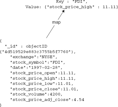
Getting back to the first task of finding the highest price for each stock in the period between 1970 and 2010, an appropriate map function could be as follows:

var map = function() {
  emit(this.stock_symbol, { stock_price_high: this.stock_price_high });
};

manipulate_nyse_market_data.txt

This function will be applied on every document in the collection. For each document, it picks up the stock_symbol as the key and emits the stock_symbol with the stock_price_high for that document as the key/value pair. Pictorially it would be as shown in Figure 11-1.

FIGURE 11-1

The key/value pair extracted in the map phase is the input for the reduce phase. In MongoDB, a reduce function is defined as a JavaScript function as follows:

MongoDB supports only JavaScript as the language to define map and reduce functions.

var reduce = function(key, values) {
  var highest_price = 0.0;
  values.forEach(function(doc) {
    if( typeof doc.stock_price_high != "undefined") {
      print("doc.stock_price_high" + doc.stock_price_high);
      if (parseFloat(doc.stock_price_high) > highest_price) { highest_price = 
parseFloat(doc.stock_price_high); print("highest_price" + highest_price); }
    }
  });
  return { highest_stock_price: highest_price };
};

manipulate_nyse_market_data.txt

The reduce function receives two arguments: a key and an array of values. In the context of the current example, a stock with symbol "FDI" will have a number of different key/value pairs from the map phase. Some of these would be as follows:

(key : "FDI", { "stock_price_high" : 11.11 })
(key : "FDI", { "stock_price_high" : 11.18 })
(key : "FDI", { "stock_price_high" : 11.08 })
(key : "FDI", { "stock_price_high" : 10.99 })
(key : "FDI", { "stock_price_high" : 10.89 })

Running a simple count as follows: db.nyse.find({stock_symbol: "FDI"}).count();, reveals that there are 5,596 records. Therefore, there must be as many key/value pairs emitted from the map phase. Some of the values for these records may be undefined, so there may not be exactly 5,596 results emitted by the map phase.

The reduce function receives the values like so:

reduce('FDI', [{stock_price_high: 11.11}, {stock_price_high: 11.18},
 {stock_price_high: 11.08}, {stock_price_high: 10.99}, ...]);

Now if you revisit the reduce function, you will notice that the passed-in array of values for each key is iterated over and a closure is called on the array elements. The closure, or inner function, carries out a simple comparison, determining the highest price for the set of values that are bound together by a common key.

The output of the reduce phase is a set of key/value pairs containing the symbol and the highest price value, respectively. There is exactly one key/value pair per stock symbol. MongoDB allows for an optional finalize function to pass the output of a reduce function and summarize it further.

Next, you set up the same data in CouchDB and carry out a few additional types of aggregation functions using MapReduce.

Uploading Historical NYSE Market Data into CouchDB

To start with, you need a script to parse the .csv files, convert .csv records to JSON documents, and then upload it to a CouchDB server. A simple sequential Python script easily gets the job done. However, being sequential in nature it crawls when trying to upload over 9 million documents. In most practical situations, you probably want a more robust parallel script to add data to a CouchDB database. For maximum efficiency, you may also want to leverage CouchDB’s bulk upload API to upload a few thousand documents at a time.

The core function of the script is encapsulated in a function named upload_nyse_market_data, which is as follows:

def upload_nyse_market_data():
    couch_server = Couch('localhost', '5984')
    print "
Create database 'nyse_db':"
    couch_server.createDb('nyse_db')
    
    for file in os.listdir(PATH):
        if fnmatch.fnmatch(file, 'NYSE_daily_prices_*.csv'):
            print "opening file: " + file 
            f = open(PATH+file, 'r' )
            reader = csv.DictReader( f )
            print "beginning to save json documents converted from csv data in 
" + file for row in reader:
                json_doc = json.dumps(row)
                couch_server.saveDoc('nyse_db', json_doc)
                print "available json documents converted from csv data in 
" + file + " saved"
                print "closing " + file
            f.close()

upload_nyse_market_data_couchdb.py

This function parses each .csv file, whose name matches a pattern as follows: 'NYSE_daily_prices_*.csv'. The Python script leverages the csv.DicReader to parse the .csv files and extract header information with ease. Then it uses the JSON module to dump a parsed record as a JSON document. The function uses a class named Couch to connect to a CouchDB server, create and delete databases, and put and delete documents. The Couch class is a simple wrapper for the CouchDB REST API and draws much inspiration from a sample wrapper illustrated in the CouchDB wiki at http://wiki.apache.org/couchdb/Getting_started_with_Python.

After the data is uploaded, you are ready to use MapReduce to run a few aggregation functions on the data. I first re-run the last query, used with MongoDB, to find the highest price for each stock for the entire period between 1970 and 2010. Right afterwards, I run another query to find the lowest price per year for each stock for the period between 1970 and 2010. As opposed to the first query, where the highest price for a stock was determined for the entire period, this second query aggregates data on two levels: year and stock.

In CouchDB, MapReduce queries that help manipulate and filter a database of documents create a view. Views are primary tools for querying and reporting on CouchDB documents. There are two types of views: permanent and temporary. I use permanent views to illustrate the examples in this section. Permanent views generate underlying data indexes that make it fast after the initial index buildup and are recommended in every production environment. Temporary views are good for ad-hoc prototyping. A view is defined within a design document. Design documents are special types of CouchDB documents that run application code. CouchDB supports the notion of multiple view servers to allow application code to be in different programming languages. This means you could write MapReduce operations for CouchDB using JavaScript, Erlang, Java, or any other supported language. I use JavaScript examples in this section to illustrate CouchDB’s MapReduce-based querying features.

A design document listed immediately after this paragraph contains three views for the following:

• Listing of all documents
• Finding the highest price for each stock for the entire period between 1970 and 2010
• Finding the lowest price per stock per year

The design document itself is as follows:

{
  "_id":"_design/marketdata",
  "language": "javascript",
  "views": {
    "all": {
      "map": "function(doc) { emit(null, doc) }"
    },
    "highest_price_per_stock": {
      "map": "function(doc) { emit(doc.stock_symbol, doc.stock_price_high) }",
      "reduce": "function(key, values) { 
        highest_price = 0.0;
        for(var i=0; i<values.length; i++) {
          if( (typeof values[i] != 'undefined') && (parseFloat(values[i]) > 
highest_price) ) {
                highest_price = parseFloat(values[i]);
          }
        }
        return highest_price;
      }"
    },
    "lowest_price_per_stock_per_year": {
      "map": "function(doc) { emit([doc.stock_symbol, doc.date.substr(0,4)], 
doc.stock_price_low) }",
      "reduce": "function(key, values) { 
        lowest_price = parseFloat(values[0]);
        for(var i=0; i<values.length; i++) {
          if( (typeof values[i] != 'undefined') && (parseFloat(values[i]) < 
lowest_price) ) {
                lowest_price = parseFloat(values[i]);
          }
        }
        return lowest_price;
      }"
    }
  }
}

mydesign.json

This design document is saved in a file named mydesign.json. The document can be uploaded to the nyse_db database as follows:

curl -X PUT http://127.0.0.1:5984/nyse_db/_design/marketdata -d @mydesign.json

CouchDB’s REST-style interaction and adherence to JSON makes editing and uploading design documents no different from managing database documents. In response to the design document upload using the HTTP PUT method you should see a response as follows:

{"ok":true,"id":"_design/marketdata","rev":"1-9cce1dac6ab04845dd01802188491459"}

The specific content of the response will vary but if you see errors you know that there is some problem with either your design document or the upload operation.

CouchDB’s web-based administration console, Futon, can be used to quickly review a design document and invoke the views to trigger the MapReduce jobs. The first MapReduce run is likely to be slow for a large data set because CouchDB is building an index for the documents based on the map function. Subsequent runs will use the index and execute much faster. Futon also provides a phased view of your map and subsequent reduce jobs and can be quite useful to understand how the data is aggregated.

In the previous example, the logic for the aggregation is quite simple and needs no explanation. However, a few aspects of the design document and the views are worth noting. First, the "language" property in the design document specifies the view server that should process this document. The application code uses JavaScript so the value for the "language" property is explicitly stated as such. If no property is stated, the value defaults to JavaScript. Do not forget to specify Erlang or Java, if that’s what you are using instead of JavaScript. Second, all view code that leverages MapReduce is contained as values of the "views" property. Third, keys for MapReduce key/value pairs don’t need to be strings only. They can be of any valid JSON type. The view that calculates the lowest price per year per stock simplifies the calculation by emitting an array of stock and year, extracted from the date property in a document, as the key. Fourth, permanent views index documents by the keys emitted in the map phase. That means if you emit a key that is an array of stock symbol and year, documents are indexed using these two properties in the given order.

You can access the view and trigger a MapReduce run. View access being RESTful can be invoked using the browser via the Futon console, via a command-line client such as curl or by any other mechanism that supports REST-based interaction.

Now that you have seen a couple of examples of MapReduce in the context of two document databases, MongoDB and CouchDB, I cover sorted ordered column-family stores.

MAPREDUCE WITH HBASE

Next, you upload the NYSE data set into an HBase instance. This time, use MapReduce itself to parse the .csv files and populate the data into HBase. Such “chained” usage of MapReduce is quite popular and serves well to parse large files. Once the data is uploaded to HBase you can use MapReduce a second time to run a few aggregate queries. Two examples of MapReduce have already been illustrated and this third one should reinforce the concept of MapReduce and demonstrate its suitability for multiple situations.

To use MapReduce with HBase you can use Java as the programming language of choice. It’s not the only option though. You could write MapReduce jobs in Python, Ruby, or PHP and have HBase as the source and/or sink for the job. In this example, I create four program elements that need to work together:

• A mapper class that emits key/value pairs.
• A reducer class that takes the values emitted from mapper and manipulates it to create aggregations. In the data upload example, the mapper only inserts the data into an HBase table.
• A driver class that puts the mapper class and the reducer class together.
• A class that triggers the job in its main method.

You can also combine all these four elements into a single class. The mapper and reducer can become static inner classes in that case. For this example, though, you create four separate classes, one each for the four elements just mentioned.

I assume Hadoop and HBase are already installed and configured. Please add the following .jar files to your Java classpath to make the following example compile and run:

• hadoop-0.20.2-ant.jar
• hadoop-0.20.2-core.jar
• hadoop-0.20.2-tools.jar
• hbase-0.20.6.jar

The hadoop jar files are available in the Hadoop distribution and the hbase jar file comes with HBase.

The mapper is like so:

package com.treasuryofideas.hbasemr;
import java.io.BufferedReader;
import java.io.FileReader;
import java.io.IOException;
 
import org.apache.hadoop.io.LongWritable;
import org.apache.hadoop.io.MapWritable;
import org.apache.hadoop.io.Text;
import org.apache.hadoop.mapreduce.Mapper;
 
public class NyseMarketDataMapper extends
    Mapper<LongWritable, Text, Text, MapWritable> {
  
  public void map(LongWritable key, MapWritable value, Context context)
      throws IOException, InterruptedException {
    
    final Text EXCHANGE = new Text("exchange");
    final Text STOCK_SYMBOL = new Text("stockSymbol");
    final Text DATE = new Text("date");
    final Text STOCK_PRICE_OPEN = new Text("stockPriceOpen");
    final Text STOCK_PRICE_HIGH = new Text("stockPriceHigh");
    final Text STOCK_PRICE_LOW = new Text("stockPriceLow");
    final Text STOCK_PRICE_CLOSE = new Text("stockPriceClose");
    final Text STOCK_VOLUME = new Text("stockVolume");
    final Text STOCK_PRICE_ADJ_CLOSE = new Text("stockPriceAdjClose");
    
    try
    {
      //sample market data csv file
      String strFile = "data/NYSE_daily_prices_A.csv";
 
      //create BufferedReader to read csv file
      BufferedReader br = new BufferedReader( new FileReader(strFile));
      String strLine = "";
      int lineNumber = 0;
 
      //read comma separated file line by line
      while( (strLine = br.readLine()) != null)
      {
        lineNumber++;
                if(lineNumber > 1) {
                  String[] data_values = strLine.split(",");
                  MapWritable marketData = new MapWritable();
                  marketData.put(EXCHANGE, new Text(data_values[0]));
                  marketData.put(STOCK_SYMBOL, new Text(data_values[1]));
                  marketData.put(DATE, new Text(data_values[2]));
                  marketData.put(STOCK_PRICE_OPEN, new Text(data_values[3]));
                  marketData.put(STOCK_PRICE_HIGH, new Text(data_values[4]));
                  marketData.put(STOCK_PRICE_LOW, new Text(data_values[5]));
                  marketData.put(STOCK_PRICE_CLOSE, new Text(data_values[6]));
                  marketData.put(STOCK_VOLUME, new Text(data_values[7]));
                  marketData.put(STOCK_PRICE_ADJ_CLOSE, new Text(data_values[8]));
                  
                  context.write(new Text(String.format("%s-%s", data_values[1], 
data_values[2])), marketData);
                  
                }  
      }
 
 
    }
    catch(Exception e)
    {
      System.errout.println("Exception while reading csv file or process 
interrupted: " + e);
    }
    
    }
}

NyseMarketDataMapper.java

The preceding code is rudimentary and focuses only on demonstrating the key features of a map function. The mapper class extends org.apache.hadoop.mapreduce.Mapper and implements the map method. The map method takes key, value, and a context object as the input parameters. In the emit method, you will notice that I create a complex key by joining the stock symbol and date together.

The .csv parsing logic itself is simple and may need to be modified to support conditions where commas appear within each data item. For the current data set, though, it works just fine.

The second part is a reducer class with a reduce method. The reduce method simply uploads data into HBase tables. The code for the reducer can be as follows:

public class NyseMarketDataReducer extends TableReducer<Text, MapWritable, 
ImmutableBytesWritable> {
         public void reduce(Text arg0, Iterable arg1, Context context) {
        //Since the complex key made up of stock symbol and date is unique
                  //one value comes for a key.
        Map marketData = null;
        for (MapWritable value : arg1) {
            marketData = value;
            break;
        }
 
        ImmutableBytesWritable key = new ImmutableBytesWritable(Bytes
                .toBytes(arg0.toString()));
        Put put = new Put(Bytes.toBytes(arg0.toString()));
        put.add(Bytes.toBytes("mdata"), Bytes.toBytes("daily"), Bytes
                .toBytes((ByteBuffer) marketData));
        try {
            context.write(key, put);
        } catch (IOException e) {
            // TODO Auto-generated catch block
        } catch (InterruptedException e) {
            // TODO Auto-generated catch block
        }
    }
 
}

NyseMarketDataReducer.java

The map function and the reduce function are tied together in a driver class as follows:

public class NyseMarketDataDriver extends Configured implements Tool {
   @Override
    public int run(String[] arg0) throws Exception {
        HBaseConfiguration conf = new HBaseConfiguration();
        Job job = new Job(conf, "NYSE Market Data Sample Application");
        job.setJarByClass(NyseMarketDataSampleApplication.class);
        job.setInputFormatClass(TextInputFormat.class);
        job.setMapperClass(NyseMarketDataMapper.class);
        job.setReducerClass(NyseMarketDataReducer.class);
        job.setMapOutputKeyClass(Text.class);
        job.setMapOutputValueClass(Text.class);
 
        FileInputFormat.addInputPath(job, new Path(
                "hdfs://localhost/path/to/NYSE_daily_prices_A.csv"));
        TableMapReduceUtil.initTableReducerJob("nysemarketdata",
                NyseMarketDataReducer.class, job);
        boolean jobSucceeded = job.waitForCompletion(true);
        if (jobSucceeded) {
            return 0;
        } else {
            return -1;
        }
    }
 
}

NyseMarketDataDriver.java

Finally, the driver needs to be triggered as follows:

package com.treasuryofideas.hbasemr;
import org.apache.hadoop.conf.Configuration;
import org.apache.hadoop.util.ToolRunner;
 
public class NyseMarketDataSampleApplication {
    public static void main(String[] args) throws Exception {
        int m_rc = 0;
        m_rc = ToolRunner.run(new Configuration(), 
new NyseMarketDataDriver(), args);
        System.exit(m_rc);
    }
 
}

NyseMarketDataSampleApplication.java

That wraps up a simple case of MapReduce with HBase. Next, you see additional use cases, which are a bit more advanced and complex than a simple HBase write.

MAPREDUCE POSSIBILITIES AND APACHE MAHOUT

MapReduce can be used to solve a number of problems. Google, Yahoo!, Facebook, and many other organizations are using MapReduce for a diverse range of use cases including distributed sort, web link graph traversal, log file statistics, document clustering, and machine learning. In addition, the variety of use cases where MapReduce is commonly applied continues to grow.

An open-source project, Apache Mahout, aims to build a complete set of scalable machine learning and data mining libraries by leveraging MapReduce within the Hadoop infrastructure. I introduce that project and cover a couple of examples from the project in this section. The motivation for covering Mahout is to jump-start your quest to explore MapReduce further. I am hoping the inspiration will help you apply MapReduce effectively for your specific and unique use case.

To get started, go to mahout.apache.org and download the latest release or the source distribution. The project is continuously evolving and rapidly adding features, so it makes sense to grab the source distribution to build it. The only tools you need, apart from the JDK, are an SVN client to download the source and Maven version 3.0.2 or higher, to build and install it.

Get the source as follows:

svn co http://svn.apache.org/repos/asf/mahout/trunk

Then change into the downloaded “trunk” source directory and run the following commands to compile and install Apache Mahout:

mvn compile
mvn install

You may also want to get hold of the Mahout examples as follows:

cd examples
mvn compile

Mahout comes with a taste-web recommender example application. You can change to the taste-web directory and run the mvn package to get the application compiled and running.

Although Mahout is a new project it contains implementations for clustering, categorization, collaborative filtering, and evolutionary programming. Explaining what these machine learning topics mean is beyond the scope of this book but I will walk through an elementary example to show Mahout in use.

Mahout includes a recommendation engine library, named Taste. This library can be used to quickly build systems that can have user-based and item-based recommendations. The system uses collaborative filtering.

Taste has five main parts, namely:

• DataModel — Model abstraction for storing Users, Items, and Preferences.
• UserSimilarity — Interface to define the similarity between two users.
• ItemSimilarity — Interface to define the similarity between two items.
• Recommender — Interface that recommendation provider implements.
• UserNeighborhood — Recommendation systems use the neighborhood for user similarity for coming up with recommendations. This interface defines the user neighborhood.

You can build a recommendation system that leverages Hadoop to run the batch computation on large data sets and allow for highly scalable machine learning systems.

Let’s consider ratings by users for a set of items is in a simple file, named ratings.csv. Each line of this file has user_id, item_id, ratings. This is quite similar to what you saw in the MovieLens data set earlier in this book. Mahout has a rich set of model classes to map this data set. You can use the FileDataModel as follows:

FileDataModel dataModel = new FileDataModel(new File(ratings.csv));

Next, you need to identify a measure of distance to see how similar two different user ratings are. The Euclidean distance is the simplest such measure and the Pearson correlation is perhaps a good normalized measure that works in many cases. To use the Pearson correlation you can configure a corresponding similarity class as follows:

UserSimilarity userSimilarity = new PearsonCorrelationSimilarity(dataModel);

Next you need to define a user neighborhood and a recommender and combine them all to generate recommendations. The code could be as follows:

//Get a neighborhood of users
UserNeighborhood neighborhood =
        new NearestNUserNeighborhood(neighborhoodSize, userSimilarity, dataModel);
//Create the recommender
Recommender recommender =
        new GenericUserBasedRecommender(dataModel, neighborhood, userSimilarity);
User user = dataModel.getUser(userId);
System.out.println("User: " + user);
//Print out the users own preferences first
TasteUtils.printPreferences(user, handler.map);
//Get the top 5 recommendations
List<RecommendedItem> recommendations =
        recommender.recommend(userId, 5);
TasteUtils.printRecs(recommendations, handler.map);

'Taste' example

This is all that is required to get a simple recommendation system up and running.

The previous example did not explicitly use MapReduce and instead worked with the semantics of a collaborative filtering-based recommendation system. Mahout uses MapReduce to get the job done and leverage the Hadoop infrastructure to compute recommendation scores in large distributed data sets, but most of the underlying infrastructures are abstracted out for you.

The chapter demonstrates a set of MapReduce cases and shows how complications of very large data sets can be carried out with elegance. No low-level API manipulation is necessary and no worries about resource deadlocks or starvation occur. In addition, keeping data and compute together reduces the effect of I/O and bandwidth limitations.

SUMMARY

MapReduce is a powerful way to process a lot of information in a fast and efficient manner. Google has used it for a lot of its heavy lifting. Google has also been gracious enough to share the underlying ideas with the research and the developer community. In addition to that, the Hadoop team has built out a very robust and scalable open-source infrastructure to leverage the processing model. Other NoSQL projects and vendors have also adopted MapReduce.

MapReduce is replacing SQL in all highly scalable and distributed models that work with immense amounts of data. Its performance and “shared nothing” model proves to be a big winner over the traditional SQL model.

Writing MapReduce programs is also relatively easy because the infrastructure handles the complexity and lets a developer focus on chains of MapReduce jobs and the application of them to processing large amounts of data. Frequently, common MapReduce jobs can be handled with a common infrastructure such as CouchDB built-in reducers or projects such as Apache Mahout. However, sometimes defining keys and working through the reduce logic could need careful attention.