Chapter 17

Tools and Utilities

WHAT’S IN THIS CHAPTER?

• Examining popular tools and utilities for monitoring and managing NoSQL products
• Surveying log processing, MapReduce management, and search related tools
• Demonstrating a few scalable and robust manageability related utilities

This book is about NoSQL and the objective from the very beginning was to get you familiar with the topic. The intent was not to make you an expert in a specific NoSQL product. The book exposed you to as many underlying concepts as possible and to the rich diversity offered by the different NoSQL products. I have achieved that initial goal and given you enough material on NoSQL so that you feel confident and comfortable about the basic building blocks of this ever-growing domain. This final chapter continues that effort to enhance your learning of NoSQL. Instead of focusing on more concepts though, this chapter presents a few interesting and important tools and utilities that you are likely to leverage as you adopt NoSQL in your technology stack. The list is by no means exhaustive or a collection of the best available products. It’s just a representative sample.

The chapter is structured around 14 different open-source and freely available use cases, tools, and utilities. Although each of these is related to NoSQL, they are independent of each other. This means you can read linearly through this chapter or choose to go to a specific page that covers a specific product as required.

The first couple of tools, especially RRDTool and Nagios, are relevant beyond NoSQL systems. They are useful for monitoring and managing all types of distributed systems.

RRDTOOL

RRDTool is a leading open-source tool for high-performance logging and the graphing of time series data. It integrates easily with shell scripts and many different scripting languages, including Python, Ruby, Perl, Lua, and Tcl. RRDTool is written in C and compiles to most platforms. It can easily run on Linux, Windows, and Mac OS X. You can download RRDTool from http://oss.oetiker.ch/rrdtool/.

RRDTool includes a database and a graph generation and rendering environment. The RRDTool database is unlike a traditional RDBMS. It’s more like a rolling log file. RRDTool serves as a very helpful monitoring tool because it can be used to capture and graph performance, usage, and utilization metrics.

Here I present a simple example to help you understand RRDTool. Say you need to capture a metric like CPU utilization on a machine that runs a NoSQL database node. You may decide to capture the utilization metric every 60 seconds (once every minute). In addition, you may want to average the utilization metric for every hour and save such calculations for a day (24 hours). You can easily store such data and graph the saved values for easy analysis.

The RRDTool database can be thought of as a storage scheme around the perimeter of a circle. This means as data gets written around a circle you eventually come back to the starting point. When you come back to the start, newer data values overwrite the old ones. This means the amount of data you store is determined up front by the total storage allocated for the database. Continuing with the circle analogy, the circumference of the circle is determined up front.

The easiest way to create an RRDTool database is via its command-line interface (CLI), which for the rudimentary CPU utilization metric example could be as follows:

rrdtool create myrrddb.rrd 
         --start 1303520400 
         --step 60 
         DS:cpu:GAUGE:120:0:100 
         RRA:AVERAGE:0.5:60:24 
         RRA:AVERAGE:0.5:1440:31

This command creates an RRDTool database named myrrddb.rrd. It creates the database by initializing it with a set of properties that define the metric it captures and how this metric gets aggregated. Parsing the command line by line is a good idea to understand all the parameters.

The start and step parameters define the start time and the interval of capture for the data-base. The time value passed, as a parameter to the start argument, is a time value represented in terms of number of seconds since epoch, which in the case of RRDTool is 1/1/1970. The step value in seconds specifies the frequency of recording and saving a metric. Because the intent is to save CPU utilization values once every minute, the step value is specified as 60 (60 seconds).

The line right after the step argument defines the metric being captured. The value DS:cpu:GAUGE:120:0:100 follows this format:

DS:variable_name:data_source_type:heartbeat:min:max

DS is a keyword that stands for data source. DS is essentially what I have been calling metric so far. variable_name identifies the data source. In the example, cpu is a variable name for holding the CPU utilization value. data_source_type defines the type of value stored for a data source. The value in this example is GAUGE. The possible values for a data_source_type are as follows:

• COUNTER — Records the rate of change over a period. The values in this case are always increasing.
• DERIVE — Similar to a COUNTER but can accept negative values.
• ABSOLUTE — Also records rate of change but the current value stored is always in relation to the last value. The current value is different from the last value. In math terms, it’s always the “delta.”
• GAUGE — Records actual value and not rate of change.

RRDTool records values at a defined interval. In the example, myrrddb.rrd would expect a CPU utilization value to be available every 60 seconds. The RRDTool database, unlike an RDBMS, expects a value to be made available at a predefined interval. This means that if it doesn’t get a value, it records it as UNDEFINED. The heartbeat value, which in the example is 120 seconds, is when the database thinks the value is not present and then records it as UNDEFINED. If values don’t come exactly as defined, RRDTool has the capability to interpolate values if the record still arrives within the heartbeat interval. The last two values, min and max, are boundary conditions for values. Data source values outside these values are recorded as UNDEFINED. In the example, I assume the CPU utilization is a percentage utilization value and therefore 0 and 100 mark the boundary conditions for such a measure.

The last two lines depict the aggregation functions on the time series data. In the database create statement in the example, the last two lines are as follows:

RRA:AVERAGE:0.5:60:24 
RRA:AVERAGE:0.5:1440:31

RRA, like DS, is another keyword. RRA stands for Round Robin Archive. The RRA definitions follow this format:

RRA:consolidation_function:xff:step:rows

consolidation_function is an aggregation function. AVERAGE, MINIMUM, MAXIMUM, and LAST could be possible consolidation_function values. In the example, two RRA definitions are included. Both average data points. Consolidation functions operate on the values captured from the data source. Therefore, in the example of CPU utilization, RRA values will be aggregates of the per-minute CPU utilization recordings. step defines the aggregation bundle and rows specifies the number of aggregated records to be saved. In the example, a value of 60 for steps implies that the average is calculated on the basis of 60 data points of the data source recordings. The recordings are every minute so this means the averages are for every hour, because an hour has 60 minutes. The number of rows to be archived is 24. Therefore, the first RRA records average CPU utilization on a per-hour basis and keeps records for a day.

The second RRA definition is an average CPU utilization for a day, and 31 days (or a month’s worth) of data is stored for this consolidation function.

RRDTool has the ability to graph the time series data it records. You can manipulate the database from shell script or from one of the popular scripting languages. You can learn about RRDTool’s capabilities and configurations at www.mrtg.org/rrdtool/. Covering all the details is certainly beyond the scope of this book.

RRDTool is a handy tool for monitoring the health of a cluster of NoSQL nodes. As an example, Hypertable leverages RRDTool for its monitoring UI. Read more about the Hypertable monitoring UI at http://code.google.com/p/hypertable/wiki/HypertableManual#Appendix_A._Monitoring_UI.

NAGIOS

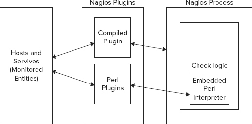
Nagios is a leading open-source hosts and services monitoring software. This powerful software application leverages a plugin architecture to provide extremely flexible and extensible monitoring infrastructure. The core of Nagios includes a monitoring process that monitors hosts or services of any type. The core process is totally unaware of what is being monitored or the meaning of the captured metrics. A plugin framework sits on top of the core process. Plugins can be compiled executables or scripts (Perl scripts and shell scripts). The plugins contain the core logic of reaching out to services and monitored entities, and measuring a specific property of that system.

A plugin checks a monitored entity and returns the results to Nagios. Nagios can process the result and take any necessary action, such as run an event handler or send a notification. Notifications and altering mechanisms serve an important function and facilitate on-time communication.

Figure 17-1 depicts the Nagios architecture.

FIGURE 17-1

Nagios can be used very effectively to monitor NoSQL databases and Hadoop clusters. A few plugins have already emerged for Hadoop and MongoDB, and Nagios can monitor Membase due to its Memcached compatibility. Plugins for other databases can also be added. Learn all about writing plugins at http://nagios.sourceforge.net/docs/nagioscore/3/en/pluginapi.html.

A GPL-licensed HDFS check plugin for Nagios is available online at www.matejunkie.com/hadoop-dfs-check-plugin-for-nagios/. A Nagios plugin to monitor MongoDB is available online at https://github.com/mzupan/nagios-plugin-mongodb.

A number of robust plugins for Nagios can help check CPU load, disk health, memory usage, and ping rates. Most protocols, including HTTP, POP3, IMAP, DHCP, and SSH can be monitored. Services in most operating systems, including Linux, Windows, and Mac OS X can be checked for their health. Read more about Nagios at www.nagios.org/.

SCRIBE

Scribe is an open-source real-time distributed log aggregator. Created at Facebook and generously open sourced by them, Scribe is a very robust and fault-tolerant system. You can download Scribe from https://github.com/facebook/scribe. Scribe is a distributed system. Each node in a cluster runs a local Scribe server and one of the nodes runs a Scribe central or master server. Logs are aggregated at the local Scribe server and sent to the central server. If the central server is down, logs are written to the local files and later sent to the central server when it’s up and running again. To avoid heavy loads on central server startup the synch is delayed for a certain time after the central server comes up.

Scribe log messages and formats are configurable. It is implemented as a Thrift service using the non-blocking C++ server.

Scribe provides a very configurable option for log writing. Messages are mapped to categories and categories are mapped to certain store types. Stores themselves can have a hierarchy. The different possible types of stores are as follows:

• File — Local file or NFS.
• Network — Send to another Scribe server.
• Buffer — Contains a primary and a secondary store. Messages are sent to primary. If primary is down, messages are sent to secondary. Messages are finally sent to primary once it’s up again.
• Bucket — Contains a large number of other stores. Creates a store hierarchy. Decides which messages to send to which stores based on a hash.
• Null — Discards all messages.
• Thriftfile — Writes messages into a Thrift TFileTransport file.
• Multi — Acts as a forwarder. Forwards messages to multiple stores.

The Thrift interface for Scribe is as follows:

enum ResultCode
{
  OK,
  TRY_LATER
}
 
struct LogEntry
{
  1:  string category,
  2:  string message
}
 
service scribe extends fb303.FacebookService
{
  ResultCode Log(1: list<LogEntry> messages);
}

A sample PHP client message could be like this:

$messages = array();
$entry = new LogEntry;
$entry->category = "test_bucket";
$entry->message = "a message";
$messages []= $entry;
$result = $conn->Log($messages);

scribe_client.php

Log parsing and management is a very important job in the world of big data and its processing. Flume is another solution like Scribe.

FLUME

Flume is a distributed service for efficiently collecting, aggregating, and moving large amounts of log data. It is based on streaming data flows. It is robust and fault tolerant and allows for flexible configurations. Flume documentation is available online at http://archive.cloudera.com/cdh/3/flume/.

Flume consists of multiple logical nodes, through which the log data flows. The nodes can be classified into three distinct tiers, which are as follows:

• Agent tier — The agent tiers usually are on nodes that generate the log files.
• Collector tier — The collector tier aggregates log data and forwards the log to the storage tiers.
• Storage tier — This could be HDFS.

The Agent tier could listen to log data from multiple tiers and sources. For example, Flume agents could listen to log files from syslog, a web server log, or Hadoop JobTracker.

Flume can be thought of as a network of logical nodes that facilitate the flow of log data from the source to the final store. Each logical node consists of a source and a sink definition. Optionally, logical nodes can have decorators. The logical node architecture allows for per-flow data guarantees like compression, durability, and batching. Each physical node is a separate Java process but multiple logical nodes can be mapped to a single physical node.

CHUKWA

Chukwa is a Hadoop subproject devoted to large-scale collection and analysis. Chukwa leverages HDFS and MapReduce to provide a scalable infrastructure to aggregate and analyze log files. Unlike Scribe and Flume, Chukwa adds an additional powerful toolkit for monitoring and analysis, beyond log collection and aggregation. For collection and aggregation, it’s quite similar to Flume.

The Chukwa architecture is shown in Figure 17-2.

FIGURE 17-2

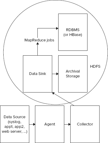
Chukwa’s reliance on the Hadoop infrastructure is its strength but it also is its weakness. As it’s currently structured, it’s meant to be a batch-oriented tool and not for real-time analysis.

Read more about Chukwa in the following presentations and research papers:

• “Chukwa: a scalable log collector” — www.usenix.org/event/lisa10/tech/slides/rabkin.pdf
• “Chukwa: A large-scale monitoring system” — www.cca08.org/papers/Paper-13-Ariel-Rabkin.pdf

PIG

Pig provides a high-level data flow definition language and environment for large-scale data analysis using MapReduce jobs. Pig includes a language, called Pig Latin, which has a simple and intuitive syntax that makes it easy to write parallel programs. The Pig layer manages efficient execution of the parallel jobs by invoking MapReduce jobs under the seams.

The MapReduce framework forces developers to think of every algorithm in terms of map and reduce functions. The MapReduce method of thinking breaks every operation into very simple operations, which go through the two steps of map and reduce. The map function emits key/value pairs of data and the reduce function runs aggregation or manipulation functions on these emitted key/value pairs. The net result of this exercise is that every join, group, average, or count operation needs to be defined every time in terms of its MapReduce equivalents. This hampers developer productivity. In terms of the Hadoop infrastructure, it also involves writing a lot of Java code. Pig provides a higher-level abstraction and provides a set of ready-to-use functions. Therefore, with Pig you no longer need to write MapReduce jobs for join, group, average, and count from the ground up. Also, the number of lines of code typically gets reduced from 100s of lines of Java code to 10s of lines of Pig Latin script.

Not only does Pig reduce the number of lines of code, but the terse and easy syntax makes it possible for non-programmers to run MapReduce jobs. As Pig evolves it becomes possible for data scientists and analysts to run complex parallel jobs without directly using a programming language.

Pig provides a language and an execution engine. The execution engine not only translates and passes over the job down to the MapReduce infrastructure but also manages the Hadoop configuration. Most often, such configuration is optimal and, therefore, Pig takes away the responsibility of optimizing configuration from you as well. This provides an extra optimization boost with no additional effort. Such optimizations involve choosing the right number of reducers or appropriate partitioning.

Interfacing with Pig

You can access the Pig engine using any of the following four mechanisms:

• Via a script
• Using the command-line interface, grunt
• Through a Java interface, the PigServer class
• With the help of an Eclipse plugin

Commands can be written using the Pig Latin scripts and then the scripts can be submitted to the Pig engine. Alternatively, you can start a Pig command-line shell, called grunt, and then use the command-line shell to interact with the Pig engine.

Although Pig takes away the effort of writing a Java program to run Hadoop MapReduce tasks, you may need to interface Pig from your Java application. In such cases, the Pig Java library classes can be used. The PigServer class allows a Java program to interface with the Pig engine via a JDBC-type interface. The usage of a Java library as opposed to an external script or program can reduce complexity, when leveraging Pig with a Java application.

Last but not least, the Pig team has created an Eclipse plugin, called PigPen, that provides a powerful IDE. The Eclipse plugin allows for graphical definition of data flow, in addition to a script development environment.

Pig Latin Basics

Pig Latin supports the following data types:

• Int
• Long
• Double
• Chararray
• Bytearray
• Map (for key/value pairs)
• Tuple (for ordered lists)
• Bag (for a set)

The best way to learn Pig Latin and how to execute Pig scripts is to work through a few examples. The Pig distribution comes with an example, complete with data and scripts. It’s available in the tutorial folder in the distribution. That is probably the best first example to start with.

The contents of the tutorial folder within the Pig distribution are as follows:

• build.xml — The ANT build script.
• data — Sample data. Contains sample data from the Excite search engine log files.
• scripts — Pig scripts.
• src — Java source.

It’s beyond the scope of this chapter or the book to get into the detailed syntax and semantics of all the Pig commands. However, I will walk through a few steps in one of the scripts in the tutorial. That should give you a flavor of Pig scripts.

You will find four scripts in the tutorial/scripts directory. These files are as follows:

• script1-hadoop.pig
• script1-local.pig
• script2-hadoop.pig
• script2-local.pig

The *-local scripts run jobs locally and the *-hadoop scripts run the job on a Hadoop cluster. The tutorial manipulates sample data from the Excite search engine log files. In script1-local.pig you will find a script that finds search phrases of a higher frequency at certain times of the day. The initial lines in this script register variables and load data for Pig. Soon after, the data is manipulated to count the frequency of n-grams. A snippet from the example is as follows:

-- Call the NGramGenerator UDF to compose the n-grams of the query.
ngramed1 = FOREACH houred GENERATE user, hour,
  flatten(
  org.apache.pig.tutorial.NGramGenerator(query))
  as ngram;
 
-- Use the DISTINCT command to get the unique n-grams for all records.
ngramed2 = DISTINCT ngramed1;
 
-- Use the GROUP command to group records by n-gram and hour.
hour_frequency1 = GROUP ngramed2 BY (ngram, hour);
 
-- Use the COUNT function to get the count (occurrences) of each n-gram.
hour_frequency2 = FOREACH hour_frequency1 GENERATE flatten($0), COUNT($1) as count;

The snippet shows sample Pig script lines. In the first of the lines, the FOREACH function helps loop through the data to generate the n-grams. In the second line, DISTINCT identifies the unique n-grams. The third line in the snippet groups the data by hour using the GROUP function. The last line in the snippet loops over the grouped data to count the frequency of occurrence of the n-grams. The FOREACH function helps loop through the data set. From the snippet it becomes evident that higher-level functions like FOREACH, DISTINCT, GROUP, and COUNT allow for easy data manipulation, without the need for detailed MapReduce functions.

Pig imposes small overheads over writing directly to MapReduce. The overhead is as low as 1.2x and so is acceptable for the comfort it offers. PigMix (http://wiki.apache.org/pig/PigMix) is a benchmarking tool that compares a task performance via Pig to direct MapReduce-based jobs.

At Yahoo!, Pig, along with Hadoop streaming is the preferred way to interact with a Hadoop cluster. Yahoo! runs one of the largest Hadoop clusters in the world and leverages this cluster for a number of mission critical features. The usage of Pig at Yahoo! testifies in favor of Pig’s production readiness.

Learn more about Pig at http://pig.apache.org/.

NODETOOL

Apache Cassandra is a popular eventually consistent data store. Its distributed nature and replication under an eventually consistent model makes it susceptible to possible complexities at run time. Having a few tools to manage and monitor the Cassandra clusters therefore comes in handy. One such command-line utility is nodetool. The nodetool utility can be run as follows:

bin/nodetool

Running it without any parameters prints out the most common choices available as command-line options. Cassandra’s distributed nodes form a ring where each node in the ring contains data that maps to a certain set of ordered tokens. All keys are hashed to tokens via MD5. To get the status of a Cassandra ring, simply run the following command:

bin/nodetool -host <host_name or ip address> ring

The host_name or ip address could be of any node in the ring. The output of this command contains the status of all nodes in a ring. It prints out the status, load, range, and an ascii art.

To get information about a particular node, run the following command:

bin/nodetool -host <host_name or ip address> info

This output of this command includes the following:

• Token
• Load info — Number of bytes of storage on disk
• Generation no — Number of times the node was started
• Uptime in seconds
• Heap memory usage

Nodetool has a number of other commands, which are as follows:

• ring — Print information on the token ring
• info — Print node information (uptime, load, and so on)
• cfstats — Print statistics on column-families
• clearsnapshot — Remove all existing snapshots
• version — Print Cassandra version
• tpstats — Print usage statistics of thread pools
• drain — Drain the node (stop accepting writes and flush all column-families)
• decommission — Decommission the node
• loadbalance — Loadbalance the node
• compactionstats — Print statistics on compactions
• disablegossip — Disable gossip (effectively marking the node dead)
• enablegossip — Reenable gossip
• disablethrift — Disable Thrift server
• enablethrift — Reenable Thrift server
• snapshot [snapshotname] — Take a snapshot using optional name snapshotname
• netstats [host] — Print network information on provided host (connecting node by default)
• move <new token> — Move node on the token ring to a new token
• removetoken status|force|<token> — Show status of current token removal, force completion of pending removal, or remove provisioned token

Learn more about nodetool at http://wiki.apache.org/cassandra/NodeTool.

OPENTSDB

As data grows and you expand your infrastructure by adding nodes to your storage and compute clusters, soon enough you have a large number of hosts, servers, and applications to manage. Most of these hosts, servers, and applications provide hooks that make them monitorable. You can ping these entities and measure their uptime, performance, usage, and other such characteristics. Capturing these metrics, especially on a frequent basis, collating them, and then analyzing them can be a complex task.

OpenTSDB is a distributed scalable time series data store that provides a flexible way to manage and monitor a vast number of hosts, servers, and applications. It uses an asynchronous way of collecting, storing, and indexing the metrics from a large number of machines. OpenTSDB is an open-source tool. The team at StumbleUpon created it. It uses HBase to store the collected data. The application allows for real-time plotting and analysis.

A high-level look at the architecture of OpenTSDB is depicted in Figure 17-3.

FIGURE 17-3

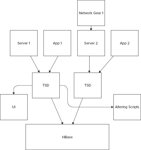
OpenTSDB has the capacity to store billions of records and so you don’t need to worry about deleting metrics and log data. Analysis can be run on this large data set to reveal interesting correlated measures, which can provide interesting insight into the working of your systems. OpenTSDB is distributed; it also avoids a single point of failure.

Learn more about OpenTSDB at http://opentsdb.net/index.html.

SOLANDRA

Lucene is a popular open-source search engine. It is written in Java and has been in use in many products and organizations for the past few years. Solr is a wrapper on top of the Lucene library. Solr provides an HTTP server, JSON, XML/HTTP support, and a bunch of other value-added features on top of Lucene. Under the seams, all of Solr’s search facility is powered by Lucene. You can learn more about Lucene at http://lucene.apache.org/java/docs/index.html and learn more about Solr at http://lucene.apache.org/solr/.

Solandra is an interesting experimental project by Jake Luciani. The Solandra project was originally introduced under the name of Lucandra, which integrated Lucene with Cassandra and used Cassandra as the data store for Lucene indexes and documents. Later, the project was moved over to support Solr, which builds on top of Lucene.

Lucene is a simple and elegant search library that can be easily integrated into your application. Its core facility manages indexes. Documents are parsed and indexed and stored away into a storage scheme, which could be a filesystem, memory, or any other store. Queries for documents are parsed by Lucene and translated into corresponding index searches. The index reader reads indexes and builds a response, which is returned to the calling party.

Solandra uses Cassandra as the storage scheme and so implements IndexWriter and IndexReader interfaces for Lucene to write indexes and documents to Cassandra. Figures 17-4 and 17-5 depict the logical architecture around index reader and writer in Solr (and Lucene) and Solandra.

FIGURE 17-4

FIGURE 17-5

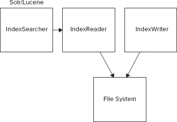
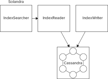
Solandra defines two column-families to store the index and the documents. The search term column-family, the one that stores index, has a key of the form indexName/field/term and the values stored in the column-family against the term are { documentId , positionVector }. The document itself is also stored, but in a separate column-family. The document column-family has a key of the form indexName/documented and the values stored against a key of this form are { fieldName , value }.

Solandra runs a Solr and Cassandra instance together on a node within the same JVM. Solandra index reader and writer performance has been observed to be slower than regular Solr, but Solandra adds the capability to scale easily. If you already use Cassandra or are having trouble scaling Solr by other means, give Solandra a try. The Solandra project is online at https://github.com/tjake/Solandra.

Similar experiments have also been carried out with HBase as the underlying storage instead of Cassandra. One such experimental project is lucehbase, which is online at https://github.com/thkoch2001/lucehbase.

If scaling Lucene is your concern and you are not a Cassandra user, I would not recommend using Solandra. I would recommend using Katta instead. Katta (http://katta.sourceforge.net/) enables storage of Lucene indexes on the Hadoop distributed filesystem, therefore providing scalable and distributed search software. It also allows you to leverage the scalable Hadoop infrastructure.

HUMMINGBIRD AND C5T

Hummingbird is actively developed real-time web traffic visualization software that uses MongoDB. It’s in the early stages of development but is so interesting and impressive that it’s worth a mention as one of the tools and utilities to watch out for.

Hummingbird is built on top of node.js and leverages web sockets to push data up to your browser. As a fallback option, Hummingbird uses Flash sockets to send the data up to the server. Twenty updates are sent per second providing a real-time view of the activity on your website. The project is open source and liberally licensed using the MIT license. It’s online at https://github.com/mnutt/hummingbird.

Node.js is an event-driven I/O framework for the V8 JavaScript engine on Linux and Unix platforms. It is intended for writing scalable network programs such as web servers. It is similar in design to and influenced by systems like Ruby’s Event Machine or Python’s Twisted. Learn more about node.js at http://nodejs.org/.

Hummingbird stores its real-time web traffic data in MongoDB, which provides fast read and write capabilities. A node.js-based tracking server records user activity on a website and stores it in a MongoDB server. A number of metrics like hits, locations, sales, and total views are implemented. As an example, the hits metric is defined as follows:

var HitsMetric = {
  name: 'Individual Hits',
  initialData: [],
  interval: 200,
  incrementCallback: function(view) {
    var value = {
      url: view.env.u,
      timestamp: view.env.timestamp,
      ip: view.env.ip
    };
    this.data.push(value);
  }
}
 
for (var i in HitsMetric)
  exports[i] = HitsMetric[i];

Learn more about Hummingbird at http://projects.nuttnet.net/hummingbird/.

C5t is another interesting piece of software built using MongoDB. It’s content management software written using TurboGears, a Python web framework, and MongoDB. The source is available online at https://bitbucket.org/percious/c5t/wiki/Home.

Typing in the desired URL can create pages. Pages can be public or private. It offers built-in authentication and authorization and full text search.

GEOCOUCH

GeoCouch is an extension to CouchDB that provides spatial index for Apache CouchDB. The project is hosted at https://github.com/couchbase/geocouch and it is included with Couchbase by Couchbase, Inc. who sponsor its development. The first version of GeoCouch used Python and SpatiaLite and interacted with CouchDB via stdin and stdout. The current version of GeoCouch is written in Erlang and integrates more elegantly with CouchDB.

Spatial indexes bring in the perspective of location to a data point. With the emergence of GPS, location-based sensors, mapping, and local searches, geospatial indexing is becoming an important part of many applications.

GeoCouch supports a number of geospatial index types:

• Point
• Polygon
• LineString
• MultiPoint
• MultiPolygon
• MultiLineString
• GeometryCollection

GeoCouch uses an R-tree data structure to store the geospatial index. R-tree (http://en.wikipedia.org/wiki/R-tree) is used in many geospatial products like PostGIS, SpatiaLite, and Oracle Spatial. The R-tree data structure uses a bounding box as an approximation to a geolocation. It is good for representing most geometries.

A good case study of GeoCouch is the PDX API (www.pdxapi.com/) that leverages GeoCouch to provide a REST service for the open geodatasets offered by the city of Portland. The city of Portland published its geodatasets as shapefiles. These shapefiles were converted to GeoJSON using PostGIS. CouchDB supports JSON and was able to easily import GeoJSON and help provide a powerful REST API with no extra effort.

ALCHEMY DATABASE

Alchemy database (http://code.google.com/p/alchemydatabase/) is a split personality database. It can act as an RDBMS and as a NoSQL product. It is built on top of Redis and Lua. Alchemy embeds a Lua interpreter as a part of the product. Because of its reliance on Redis, the database is very fast and tries to do most operations in memory. However, this also means it shares the limitations of Redis when it comes to having a big divergence between the working set in memory and the entire data set on disk.

Alchemy achieves impressive performance because:

• It uses an event-driven network server that leverages memory as much as possible.
• Efficient data structures and compression help store a lot of data efficiently in RAM.
• The most relevant SQL statements for OLTP are supported, keeping the system lightweight and still useful. Every complex SQL statement is not supported. The list of supported SQL commands is available online at http://code.google.com/p/alchemydatabase/wiki/CommandReference#Supported_SQL.

WEBDIS

Webdis (http://webd.is) is a fast HTTP interface for Redis. It’s a simple HTTP web server that sends requests down to Redis and sends responses back to the client. By default, Webdis supports JSON but it also supports other formats, which are as follows:

• Text, served as text/plain
• HTML, XML, PNG, JPEG, PDF served with their extensions
• BSON, served as application/bson
• Raw Redis protocol format

Webdis acts like a regular web server, but of course with a few modifications it supports all those commands that Redis can respond to. Regular requests are responded to with a 200 ok code. If access control doesn’t allow a response to a request, the client receives a 403 forbidden HTTP response. GET, POST, and OPTIONS are not allowed and so return 405 Method Not Allowed. Webdis supports HTTP PUT and value can be set with a command as follows:

curl --upload-file my-data.bin http://127.0.0.1:7379/SET/akey

SUMMARY

As I write the summary to this last chapter, I hope you had an enjoyable and enriching experience learning the details of an emerging and important technology. This chapter presents a few use cases, tools, and utilities that relate to NoSQL.

Tools like RRDTool and Nagios are general purpose and are valuable additions to any monitoring and management software. Tools like nodetool add value when it comes to specifically managing and monitoring Cassandra.

Scribe, Flume, and Chukwa provide powerful capabilities around distributed log processing and aggregation. They provide a very robust function to help manage the large number of log files that are generated in any distributed environment. OpenTSDB provides a real-time infrastructure for monitoring hosts, services, and applications.

Pig is a valuable tool for writing smart MapReduce jobs on a Hadoop cluster. The chapter gets you started with it. Interesting applications like Solandra, Hummingbird, c5t, GeoCouch, Alchemy database, and Webdis demonstrate what you can do when you combine the flexibility and power of NoSQL products with your interesting ideas. The list of use cases, tools, and utilities covered in this chapter are not exhaustive but only a small sample. After reading through this book, I hope you are inspired to learn more of the specific NoSQL products that seem most interesting and most appropriate for your context.