
Chapter 12
Analyzing Big Data with Hive
WHAT’S IN THIS CHAPTER?
- Introducing Apache Hive, a data warehousing infrastructure built on top of Hadoop
- Learning Hive with the help of examples
- Exploring Hive commands syntax and semantics
- Using Hive to query the MovieLens data set
Solutions to big data-centric problems involve relaxed schemas, column-family-centric storage, distributed filesystems, replication, and sometimes eventual consistency. The focus of these solutions is managing large, spare, denormalized data volumes, which is typically over a few terabytes in size. Often, when you are working with these big data stores you have specific, predefined ways of analyzing and accessing the data. Therefore, ad-hoc querying and rich query expressions aren’t a high priority and usually are not a part of the currently available solutions. In addition, many of these big data solutions involve products that are rather new and still rapidly evolving. These products haven’t matured to a point where they have been tested across a wide range of use cases and are far from being feature-complete. That said, they are good at what they are designed to do: manage big data.
In contrast to the new emerging big data solutions, the world of RDBMS has a repertoire of robust and mature tools for administering and querying data. The most prominent and important of these is SQL. It’s a powerful and convenient way to query data: to slice, dice, aggregate, and relate data points within a set. Therefore, as ironic as it may sound, the biggest missing piece in NoSQL is something like SQL.
In wake of the need to have SQL-like syntax and semantics and the ease of higher-level abstractions, Hive and Pig come to the rescue. Apache Hive is a data-warehousing infrastructure built on top of Hadoop, and Apache Pig is a higher-level language for analyzing large amounts of data. This chapter illustrates Hive and Pig and shows how you could leverage these tools to analyze large data sets.
Google App Engine (GAE) provides a SQL-like querying facility by offering GQL.
Before you start learning Hive, you need to install and set it up. Hive leverages a working Hadoop installation so install Hadoop first, if you haven’t already. Hadoop can be downloaded from hadoop.apache.org (read Appendix A if you need help with installing Hadoop). Currently, Hive works well with Java 1.6 and Hadoop 0.20.2 so make sure to get the right versions for these pieces of software. Hive works without problems on Mac OS X and any of the Linux variants. You may be able to run Hive using Cygwin on Windows but I do not cover any of that in this chapter. If you are on Windows and do not have access to a Mac OS X or Linux environment, consider using a virtual machine with VMware Player to get introduced to Hive. Please read Appendix A to find out how to access and install a virtual machine for experimentation.
Installing Hive is easy. Just carry out the following steps:
1. Download a stable release version of Hive. You can download hive-0.6.0 on Mac OS X using curl -O http://mirror.candidhosting.com/pub/apache//hive/hive-0.6.0/hive-0.6.0.tar.gz. On Linux and its variants use wget instead of curl.
2. Extract the distribution, available as a compressed archive. On Mac OS X and Linux, extract as follows: tar zxvf hive-0.6.0.tar.gz.
3. Set up the HIVE_HOME environment variable to point to the Hive installation directory.
4. Add $HIVE_HOME/bin to the PATH environment variable so that Hive executables are accessible from outside their home directory.
5. Start Hadoop daemons by running bin/start-all.sh from within the $HADOOP_HOME directory. This should start HDFS namenode, secondary namenode, and datanode. It should also start the MapReduce job tracker and task tracker. Use the jps command to verify that these five processes are running.
6. Create /tmp and /user/hive/warehouse folders on HDFS as follows:
bin/hadoop fs -mkdir /tmp
bin/hadoop fs -mkdir /user/hive/warehouse
The /user/hive/warehouse is the hive metastore warehouse directory.
7. Set write permission to the group on /tmp and /user/hive/warehouse folders created in HDFS. Permissions can be modified using the chmod command as follows:
bin/hadoop fs -chmod g+w /tmp
bin/hadoop fs -chmod g+w /user/hive/warehouse
If you followed through all the preceding steps, you are all set to use your Hadoop cluster for Hive. Fire up the Hive command-line interface (CLI) by running bin/hive in the $HIVE_HOME directory. Working with the Hive CLI will give you sense of déjà vu, because the semantics and syntax are quite similar to what you may have experienced with a command-line client connecting to an RDBMS.
In my pseudo-distributed local installation, bin/start-all.sh spawns five Java processes for the HDFS and MapReduce daemons.
Start out by listing the existing tables as follows:
SHOW TABLES;
hive_examples.txt
No tables have been created yet, so you will be greeted with an empty OK and a metric showing the time it took the query to run. As with most database CLI(s), the time taken metric is printed out for all queries. It’s a good first indicator of whether a query is running efficiently.
HIVE IS NOT FOR REAL-TIME QUERYING
Hive provides an elegant SQL-like query framework on top of Hadoop. Hadoop is a scalable infrastructure that can manipulate very large and distributed data sets. Therefore, Hive provides a powerful abstraction for querying and manipulating large data sets. It leverages HDFS and MapReduce.
However, Hive is not a real-time query system. It is best used as a batch-oriented tool. Hive’s dependency on the underlying Hadoop infrastructure and the MapReduce framework causes substantial overheads around job submission and scheduling. This means Hive query responses usually have high latency. As you go through the examples and try out Hive using the CLI you will notice that time taken to execute a query, even with small data sets, is in seconds and at times in minutes. This is in sharp contrast to the time taken for similar queries in RDBMS. There is no query caching in Hive so even repeat queries require as much time as the first one.
As data sets become bigger the Hive overhead is often dwarfed by the large-scale efficiencies of Hadoop. Much like a traditional RDBMS may fall back to table scans if a query is likely to touch every row, with extremely large data sets and for batch processing Hive’s performance is optimal.
Next, create a table like so:
CREATE TABLE books (isbn INT, title STRING);
hive_examples.txt
This creates a table of books, with two columns: isbn and title. The column data types are integer and string, respectively. To list the books table’s schema, query as follows:
hive> DESCRIBE books;
OK
Isbn    int
Title   string
Time taken: 0.263 seconds
hive_examples.txt
Create another table named users as follows:
CREATE TABLE users (id INT, name STRING) PARTITIONED BY (vcol STRING);
hive_examples.txt
The users table has three columns: id, name, and vcol. You can confirm this running the DESCRIBE table query as follows:
hive> DESCRIBE users;
OK
Id     int
Name   string
Vcol   string
Time taken: 0.12 seconds
hive_examples.txt
The column vcol is a virtual column. It’s a partition column derived from the partition in which the data is stored and not from the data set itself. A single table can be partitioned into multiple logical parts. Each logical part can be identified by a specific value for the virtual column that identifies the partition.
Now run the SHOW TABLES command to list your tables like so:
hive> SHOW TABLES;
OK
books
users
Time taken: 0.087 seconds
hive_examples.txt
A books table stores data about books. The isbn and title columns in the books table identify and describe a book, but having only these two properties is rather minimalistic. Adding an author column and possibly a category column to the books table seems like a good idea. In the RDBMS world such manipulations are done using the ALTER TABLE command. Not surprisingly, Hive has a similar syntax. You can modify the books table and add columns as follows:
ALTER TABLE books ADD COLUMNS (author STRING, category STRING);
hive_examples.txt
Reconfirm that the books table has a modified schema like so:
hive> DESCRIBE books;
OK
Isbn   int
Title  string
Author string
Category     string
Time taken: 0.112 seconds
hive_examples.txt
Next, you may want to modify the author column of the books table to accommodate cases where a book is written by multiple authors. In such a case, an array of strings better represents the data than a single string does. When you make this modification you may also want to attach a comment to the column suggesting that the column holds multi-valued data. You can accomplish all of this as follows:
ALTER TABLE books CHANGE author author ARRAY<STRING> COMMENT "multi-valued";
hive_examples.txt
Rerunning DESCRIBE TABLE for books, after the author column modification, produces the following output:
hive> DESCRIBE books;
OK
Isbn   int
Title  string
Author array<string>     multi-valued
Category     string
Time taken: 0.109 seconds
hive_examples.txt
The ALTER TABLE command allows you to change the properties of a table’s columns using the following syntax:
ALTER TABLE table_name CHANGE [COLUMN]
old_column_name new_column_name column_type
[COMMENT column_comment]
[FIRST|AFTER column_name]
The argument of the ALTER TABLE for a column change needs to appear in the exact order as shown. The arguments in square brackets ([]) are optional but everything else needs to be included in the correct sequence for the command to work. As a side effect, this means you need to state the same column name in succession twice when you don’t intend to rename it but intend to change only its properties. Look at the author column in the previous example to see how this impacts the command. Hive supports primitive and complex data types. Complex types can be modeled in Hive using maps, arrays, or a struct. In the example just illustrated, the column is modified to hold an ARRAY of values. The ARRAY needs an additional type definition for its elements. Elements of an ARRAY type cannot contain data of two different types. In the case of the author column, the ARRAY contains only STRING type.
Next, you may want to store information on publications like short stories, magazines, and others in addition to books and so you may consider renaming the table to published_contents instead. You could do that as follows:
ALTER TABLE books RENAME TO published_contents;
hive_examples.txt
Running DESCRIBE TABLE on published_contents produces the following output:
hive> DESCRIBE published_contents;
OK
isbn   int
title  string
author  array<string>   multi-valued
category   string
Time taken: 0.136 seconds
hive_examples.txt
Obviously, running DESCRIBE TABLE on books now returns an error:
hive> DESCRIBE books;
FAILED: Execution Error, return code 1 from org.apache.hadoop.hive.ql.exec.DDLTask
hive_examples.txt
Next, I walk through a more complete example to illustrate Hive’s querying capabilities. Because the published_contents and users tables may not be needed in the rest of this chapter, I could drop those tables as follows:
DROP TABLE published_contents;
DROP TABLE users;
In Chapter 6, you learned about querying NoSQL stores. In that chapter, I leveraged a freely available movie ratings data set to illustrate the query mechanisms available in NoSQL stores, especially in MongoDB. Let’s revisit that data set and use Hive to manipulate it. You may benefit from reviewing the MovieLens example in Chapter 6 before you move forward.
You can download the movie lens data set that contains 1 million ratings with the following command:
curl -O http://www.grouplens.org/system/files/million-ml-data.tar__0.gz
Extract the tarball and you should get the following files:
- README
- movies.dat
- ratings.dat
- users.dat
The ratings.dat file contains rating data where each line contains one rating data point. Each data point in the ratings file is structured in the following format: UserID::MovieID::Rating::Timestamp.
The ratings, movie, and users data in the movie lens data set is separated by ::. I had trouble getting the Hive loader to correctly parse and load the data using this delimiter. So, I chose to replace :: with # throughout the file. I simply opened the file in vi and replaced all occurrences of ::, the delimiter, with # using the following command:
:%s/::/#/g
Once the delimiter was modified I saved the results to new files, each with .hash_delimited appended to their old names. Therefore, I had three new files:
- ratings.dat.hash_delimited
- movied.dat.hash_delimited
- users.dat.hash_delimited
I used the new files as the source data. The original .dat files were left as is.
Load the data into a Hive table that follows the same schema as in the downloaded ratings data file. That means first create a Hive table with the same schema:
hive> CREATE TABLE ratings(
    > userid INT,
    > movieid INT,
    > rating INT,
    > tstamp STRING)
    > ROW FORMAT DELIMITED
    > FIELDS TERMINATED BY '#'

    > STORED AS TEXTFILE;
OK
Time taken: 0.169 seconds
hive_movielens.txt
Hive includes utilities to load data sets from flat files using the LOAD DATA command. The source could be the local filesystem or an HDFS volume. The command signature is like so:
LOAD DATA LOCAL INPATH <'path/to/flat/file'> OVERWRITE INTO TABLE <table name>;
No validation is performed at load time. Therefore, it’s a developer’s responsibility to ensure that the flat file data format and the table schema match. The syntax allows you to specify the source as the local filesystem or HDFS. Essentially, specifying LOCAL after LOAD DATA tells the command that the source is on the local filesystem. Not including LOCAL means that the data is in HDFS. When the flat file is in HDFS, the data is copied only into the Hive HDFS namespace. The operation is an HDFS file move operation and so it is much faster than a data load operation from the local filesystem. The data loading command also enables you to overwrite data into an existing table or append to it. The presence and absence of OVERWRITE in the command suggests overwrite and append, respectively.
The movie lens data is downloaded to the local filesystem. A slightly modified copy of the data is prepared by replacing the delimiter :: with #. The prepared data set is loaded into the Hive HDFS namespace. The command for data loading is as follows:
hive> LOAD DATA LOCAL INPATH '/path/to/ratings.dat.hash_delimited'
    > OVERWRITE INTO TABLE ratings;
Copying data from file:/path/to/ratings.dat.hash_delimited
Loading data to table ratings
OK
Time taken: 0.803 seconds
hive_movielens.txt
The movie lens ratings data that was just loaded into a Hive table contains over a million records. You could verify that using the familiar SELECT COUNT idiom as follows:
hive> SELECT COUNT(*) FROM ratings;
Total MapReduce jobs = 1
Launching Job 1 out of 1
Number of reduce tasks determined at compile time: 1
In order to change the average load for a reducer (in bytes):
  set hive.exec.reducers.bytes.per.reducer=<number>
In order to limit the maximum number of reducers:
  set hive.exec.reducers.max=<number>
In order to set a constant number of reducers:
  set mapred.reduce.tasks=<number>
Starting Job = job_201102211022_0012, Tracking URL =
http://localhost:50030/jobdetails.jsp?jobid=job_201102211022_0012
Kill Command = /Users/tshanky/Applications/hadoop/bin/../bin/hadoop job  -
Dmapred.job.tracker=localhost:9001 -kill job_201102211022_0012
2011-02-21 15:36:50,627 Stage-1 map = 0%,  reduce = 0%
2011-02-21 15:36:56,819 Stage-1 map = 100%,  reduce = 0%
2011-02-21 15:37:01,921 Stage-1 map = 100%,  reduce = 100%
Ended Job = job_201102211022_0012
OK
1000209
Time taken: 21.355 seconds
hive_movielens.txt
The output confirms that more than a million ratings records are in the table. The query mechanism confirms that the old ways of counting in SQL work in Hive. In the counting example, I liberally included the entire console output with the SELECT COUNT command to bring to your attention a couple of important notes, which are as follows:
- Hive operations translate to MapReduce jobs.
- The latency of Hive operation responses is relatively high. It took 21.355 seconds to run a count. An immediate re-run does no better. It again takes about the same time, because no query caching mechanisms are in place.
Hive is capable of an exhaustive set of filter and aggregation queries. You can filter data sets using the WHERE clause. Results can be grouped using the GROUP BY command. Distinct values can be listed with the help of the DISTINCT parameter and two tables can be combined using the JOIN operation. In addition, you could write custom scripts to manipulate data and pass that on to your map and reduce functions.
To learn more about Hive’s capabilities and its powerful query mechanisms, let’s also load the movies and users data sets from the movie lens data set into corresponding tables. This would provide a good sample set to explore Hive features by trying them out against this data set. Each row in the movies data set is in the following format: MovieID::Title::Genres. MovieID is an integer and Title is a string. Genres is also a string. The Genres string contains multiple values in a pipe-delimited format. In the first pass, you create a movies table as follows:
As with the ratings data, the original delimiter in movies.dat is changed from :: to #.
hive> CREATE TABLE movies(
    > movieid INT,
    > title STRING,
    > genres STRING)
    > ROW FORMAT DELIMITED
    > FIELDS TERMINATED BY '#'
    > STORED AS TEXTFILE;
OK
Time taken: 0.075 seconds
hive_movielens.txt
Load the flat file data into the movies table as follows:
hive> LOAD DATA LOCAL INPATH '/path/to/movies.dat.hash_delimited'
    > OVERWRITE INTO TABLE movies;
The genres string data contains multiple values. For example, a record could be as follows: Animation|Children's|Comedy. Therefore, storing this data as an ARRAY is probably a better idea than storing it as a STRING. Storing as ARRAY allows you to include these values in query parameters more easily than if they are part of a string. Splitting and storing the genres record as a collection can easily be achieved by using Hive’s ability to take delimiter parameters for collections and map keys. The modified Hive CREATE TABLE and LOAD DATA commands are as follows:
hive> CREATE TABLE movies_2(
    > movieid INT,
    > title STRING,
    > genres ARRAY<STRING>)
    > ROW FORMAT DELIMITED
    > FIELDS TERMINATED BY '#'
    > COLLECTION ITEMS TERMINATED BY '|'
    > STORED AS TEXTFILE;
OK
Time taken: 0.037 seconds
hive> LOAD DATA LOCAL INPATH '/path/to/movies.dat.hash_delimited'
    > OVERWRITE INTO TABLE movies_2;
Copying data from file:/path/to/movies.dat.hash_delimited
Loading data to table movies_2
OK
Time taken: 0.121 seconds
hive_movielens.txt
After the data is loaded, print out a few records using SELECT and limit the result set to five records using LIMIT as follows:
hive> SELECT * FROM movies_2 LIMIT 5;
OK
1      Toy Story (1995)     ["Animation","Children's","Comedy"]
2      Jumanji (1995)       ["Adventure","Children's","Fantasy"]
3      Grumpier Old Men (1995)     ["Comedy","Romance"]
4      Waiting to Exhale (1995)    ["Comedy","Drama"]
5      Father of the Bride Part II (1995)     ["Comedy"]
Time taken: 0.103 seconds
hive_movielens.txt
The third data set in the movie lens data bundle is users.dat. A row in the users data set is of the following format: UserID::Gender::Age::Occupation::Zip-code. A sample row is as follows:
1::F::1::10::48067
The values for the gender, age, and occupation properties belong to a discrete domain of possible values. Gender can be male or female, denoted by M and F, respectively. Age is represented as a step function with the value representing the lowest value in the range. All ages are rounded to the closest year and ranges are exclusive. The occupation property value is a discrete numeric value that maps to a specific string value. The occupation property can have 20 possible values as follows:
- 0: other or not specified
- 1: academic/educator
- 2: artist
- 3: clerical/admin
- 4: college/grad student
- 5: customer service
- 6: doctor/health care
- 7: executive/managerial
- 8: farmer
- 9: homemaker
- 10: K-12 student
- 11: lawyer
- 12: programmer
- 13: retired
- 14: sales/marketing
- 15: scientist
- 16: self-employed
- 17: technician/engineer
- 18: tradesman/craftsman
- 19: unemployed
- 20: writer
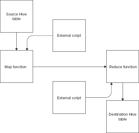
You may benefit from storing the occupation strings instead of the numeric values because it becomes easier for someone browsing through the data set to understand the data points. To manipulate the data as required, you can leverage an external script in association with the data load operations. Hive enables pluggability of external functions with map and reduce functions. The concept of plugging external scripts with map and reduce functions, involved while copying data from one Hive table to another Hive table, is summarized in Figure 12-1.
To see an external script in action, especially one that replaces occupation numbers with its string counterparts in the users table, you must first create the users table and load data into it. You can create the users table as follows:
hive> CREATE TABLE users(
    > userid INT,
    > gender STRING,
    > age INT,
    > occupation INT,
    > zipcode STRING)
    > ROW FORMAT DELIMITED
    > FIELDS TERMINATED BY '#'
    > STORED AS TEXTFILE;
hive_movielens.txt
and load users data into this table as follows:
hive> LOAD DATA LOCAL INPATH '/path/to/users.dat.hash_delimited'
    > OVERWRITE INTO TABLE users;
Next, create a second users table, users_2, and load data from the users table into this second table. During loading, leverage an external script, occupation_mapper.py, to map occupation integer values to their corresponding string values and load the string values into users_2. The code for this data transformation is as follows:
hive> CREATE TABLE users_2(
    > userid INT,
    > gender STRING,
    > age INT,
    > occupation STRING,
    > zipcode STRING)
    > ROW FORMAT DELIMITED
    > FIELDS TERMINATED BY '#'
    > STORED AS TEXTFILE;
OK
Time taken: 0.359 seconds
hive> add FILE
/Users/tshanky/workspace/hadoop_workspace/hive_workspace/occupation_mapper.py;
hive> INSERT OVERWRITE TABLE users_2
    > SELECT
    > TRANSFORM (userid, gender, age, occupation, zipcode)
    > USING 'python occupation_mapper.py'
    > AS (userid, gender, age, occupation_str, zipcode)
    > FROM users;
hive_movielens.txt
The occupation_mapper.py script is as follows:
occupation_dict = { 0:  "other or not specified",
  1:  "academic/educator",
  2:  "artist",
  3:  "clerical/admin",
  4:  "college/grad student",
  5:  "customer service",
  6:  "doctor/health care",
  7:  "executive/managerial",
  8:  "farmer",
  9:  "homemaker",
  10:  "K-12 student",
  11:  "lawyer",
  12:  "programmer",
  13:  "retired",
  14:  "sales/marketing",
  15:  "scientist",
  16:  "self-employed",
  17:  "technician/engineer",
  18:  "tradesman/craftsman",
  19:  "unemployed",
  20:  "writer"
}

for line in sys.stdin:
  line = line.strip()
  userid, gender, age, occupation, zipcode = line.split('#')
  occupation_str = occupation_map[occupation]
  print '#'.join([userid, gender, age, occupation_str, zipcode])
occupation_mapper.py
The transformation script is fairly self-explanatory. Each value from the users table is transformed using the Python script to replace occupation integer values with the corresponding string values by looking it up in the occupation_dict dictionary.
When the data is loaded and ready you can use Hive to run your good old SQL queries.
SQL has many good features but the ability to filter data using the WHERE clause is probably the most used and appreciated of them all. In this section you see how Hive matches up on its ability to support the WHERE clause.
First, get a set of any five movies from the movies table. You could use the LIMIT function to get only five records as follows:
SELECT * FROM movies LIMIT 5;
hive_movielens.txt
For me the five records were:
1     Toy Story (1995)    Animation|Children's|Comedy
2     Jumanji (1995)     Adventure|Children's|Fantasy
3     Grumpier Old Men (1995)     Comedy|Romance
4     Waiting to Exhale (1995)     Comedy|Drama
5     Father of the Bride Part II (1995)     Comedy
To list all ratings that relate to Toy Story (1995) with a movie ID of 1 use a Hive QL, the Hive query language, and query as follows:
hive> SELECT * FROM ratings
    > WHERE movieid = 1;
hive_movielens.txt
Movie IDs are numbers so to get a count of ratings for all movies with an ID lower than 10, you could use a Hive QL as follows:
hive> SELECT COUNT(*) FROM ratings
    > WHERE movieid < 10;
hive_movielens.txt
The output after a MapReduce job run is 5,290.
To find out how many users rated Toy Story (1995) as a good movie and gave it 5 out of 5 on the rating scale, you can query as follows:
hive> SELECT COUNT(*) FROM ratings
    > WHERE movieid = 1 and rating = 5;
hive_movielens.txt
This shows a case in which more than one condition is used in the WHERE clause. You could use DISTINCT in SELECT clauses to get only unique values. The default behavior is to return duplicates.
There is no LIKE operation with SELECT to allow approximate matches with the records. However, a SELECT clause allows regular expressions to be used in conjunction with column names and WHERE clause values. To select all movies that have a title that starts with the word Toy, you can query as follows:
hive> SELECT title FROM movies
    > WHERE title = `^Toy+`;
hive_movielens.txt
Notice that the regular expression is specified within backquotes. The regular expression follows the Java regular expression syntax. The regular expression facility can also be used for projection where only specific columns from a result can be returned. For example, you could return only those columns that end with the character’s ID as follows:
hive> SELECT `*+(id)` FROM ratings
    > WHERE movieid = 1;
hive_movieslens.txt
The MovieLens ratings table has rating values for movies. A rating is a numerical value that can be anything between 1 and 5. If you want to get a count of the different ratings for Toy Story (1995), with movieid = 1, you can query using GROUP BY as follows:
hive> SELECT ratings.rating, COUNT(ratings.rating)
    > FROM ratings
    > WHERE movieid = 1
    > GROUP BY ratings.rating;
hive_movieslens.txt
The output is as follows:
1     16
2     61
3     345
4     835
5     820
Time taken: 24.908 seconds
You can include multiple aggregation functions, like count, sum, and average, in a single query as long as they all operate on the same column. You are not allowed to run aggregation functions on multiple columns in the same query.
To run aggregation at the map level, you could set hive.map.aggr to true and run a count query as follows:
set hive.map.aggr=true;
SELECT COUNT(*) FROM ratings;
Hive QL also supports ordering of result sets in ascending and descending order using the ORDER BY clause. To get all records from the movies tables ordered by movieid in descending order, you can query as follows:
hive> SELECT * FROM movies
    > ORDER BY movieid DESC;
hive_movielens.txt
Hive has another ordering facility. It’s SORT BY, which is similar to ORDER BY in that it orders records in ascending or descending order. However, unlike ORDER BY, SORT BY applies ordering on a per-reducer basis. This means the final result set may be partially ordered. All records managed by the same reducer will be ordered but records across reducers will not be ordered.
Hive allows partitioning of data sets on the basis of a virtual column. You can distribute partitioned data to separate reducers by using the DISTRIBUTE BY method. Data distributed to different reducers can be sorted on a per-reducer basis. Shorthand for DISTRIBUTE BY and ORDER BY together is CLUSTER BY.
Hive QL’s SQL-like syntax and semantics is very inviting for developers who are familiar with RDBMS and SQL and want to explore the world of large data processing with Hadoop using familiar tools. SQL developers who start exploring Hive soon start craving their power tool: the SQL join. Hive doesn’t disappoint even in this facility. Hive QL supports joins.
Hive supports equality joins, outer joins, and left semi-joins. To get a list of movie ratings with movie titles you can obtain the result set by joining the ratings and the movies tables. You can query as follows:
hive> SELECT ratings.userid, ratings.rating, ratings.tstamp, movies.title
    > FROM ratings JOIN movies
    > ON (ratings.movieid = movies.movieid)
    > LIMIT 5;
The output is as follows:
376    4     980620359     Toy Story (1995)
1207   4     974845574     Toy Story (1995)
28     3     978985309     Toy Story (1995)
193    4     1025569964    Toy Story (1995)
1055   5     974953210     Toy Story (1995)
Time taken: 48.933 seconds
Joins are not restricted to two tables only. You can join more than two tables. To get a list of all movie ratings with movie title and user gender — the gender of the person who rated the movies — you can join the ratings, movies, and users tables. The query is as follows:
hive> SELECT ratings.userid, ratings.rating, ratings.tstamp, movies.title,
 users.gender
    > FROM ratings JOIN movies ON (ratings.movieid = movies.movieid)
    > JOIN users ON (ratings.userid = users.userid)
    > LIMIT 5;
The output is as follows:
1  3  978300760  Wallace & Gromit: The Best of Aardman Animation (1996)  F
1  5  978824195  Schindler's List (1993)  F
1  3  978301968  My Fair Lady (1964)  F
1  4  978301398  Fargo (1996)  F
1  4  978824268  Aladdin (1992)  F
Time taken: 84.785 seconds
The data was implicitly ordered so you receive all the values for females first. If you wanted to get only records for male users, you would modify the query with an additional WHERE clause as follows:
hive> SELECT ratings.userid, ratings.rating, ratings.tstamp, movies.title,
users.gender
    > FROM ratings JOIN movies ON (ratings.movieid = movies.movieid)
    > JOIN users ON (ratings.userid = users.userid)
    > WHERE users.gender = 'M'
    > LIMIT 5;
The output this time is as follows:
2  5  978298625  Doctor Zhivago (1965)  M
2  3  978299046  Children of a Lesser God (1986)  M
2  4  978299200  Kramer Vs. Kramer (1979)  M
2  4  978299861  Enemy of the State (1998)  M
2  5  978298813  Driving Miss Daisy (1989)  M
Time taken: 80.769 seconds
Hive supports more SQL-like features including UNION and sub-queries. For example, you could combine two result sets using the UNION operation as follows:
select_statement UNION ALL select_statement UNION ALL select_statement ...
You can query and filter the union of SELECT statements further. A possible simple SELECT could be as follows:
SELECT *
FROM (
  select_statement
  UNION ALL
  select_statement
) unionResult
Hive also supports sub-queries in FROM clauses. A possible example query to get a list of all users who have rated more than fifteen movies as the very best, with rating value 5, is as follows:
hive> SELECT user_id, rating_count
    > FROM (SELECT ratings.userid as user_id, COUNT(ratings.rating) as
rating_count
    > FROM ratings
    > WHERE ratings.rating = 5
    > GROUP BY ratings.userid ) top_raters
    > WHERE rating_count > 15;
There is more to Hive and its query language than what has been illustrated so far. However, this may be a good logical point to wrap up. The chapter so far has established that Hive QL is like SQL and fills the gap that RDBMS developers feel as soon as they start with NoSQL stores. Hive provides the right abstraction to make big data processing accessible to a larger number of developers.
Before I conclude the chapter, though, a couple of more aspects need to be covered for completeness. First, a short deviation into explain plans provides a way of peeking into the MapReduce behind a query. Second, a small example is included to show a case for data partitioning.
Explain Plan
Most RDBMSs include a facility for explaining a query’s processing details. They usually detail aspects like index usage, data points accessed, and time taken for each. The Hadoop infrastructure is a batch processing system that leverages MapReduce for distributed large-scale processing. Hive builds on top of Hadoop and leverages MapReduce. An explain plan in Hive reveals the MapReduce behind a query.
A simple example could be as follows:
hive> EXPLAIN SELECT COUNT(*) FROM ratings
    > WHERE movieid = 1 and rating = 5;
OK
ABSTRACT SYNTAX TREE:
  (TOK_QUERY (TOK_FROM (TOK_TABREF ratings))
(TOK_INSERT (TOK_DESTINATION (TOK_DIR TOK_TMP_FILE))
(TOK_SELECT (TOK_SELEXPR (TOK_FUNCTIONSTAR COUNT)))
(TOK_WHERE (and (= (TOK_TABLE_OR_COL movieid) 1)
(= (TOK_TABLE_OR_COL rating) 5)))))
STAGE DEPENDENCIES:
  Stage-1 is a root stage
  Stage-0 is a root stage

STAGE PLANS:
  Stage: Stage-1
    Map Reduce
      Alias -> Map Operator Tree:
        ratings
          TableScan
            alias: ratings
            Filter Operator
              predicate:
                  expr: ((movieid = 1) and (rating = 5))
                  type: boolean
              Filter Operator
                predicate:
                    expr: ((movieid = 1) and (rating = 5))
                    type: boolean
                Select Operator
                  Group By Operator
                    aggregations:
                          expr: count()
                    bucketGroup: false
                    mode: hash
                    outputColumnNames: _col0
                    Reduce Output Operator
                      sort order:
                      tag: -1
                      value expressions:
                            expr: _col0
                            type: bigint
      Reduce Operator Tree:
        Group By Operator
          aggregations:
                expr: count(VALUE._col0)
          bucketGroup: false
          mode: mergepartial
          outputColumnNames: _col0
          Select Operator
            expressions:
                  expr: _col0
                  type: bigint
            outputColumnNames: _col0
            File Output Operator
              compressed: false
              GlobalTableId: 0
              table:
                  input format: org.apache.hadoop.mapred.TextInputFormat
                  output format:
org.apache.hadoop.hive.ql.io.HiveIgnoreKeyTextOutputFormat

  Stage: Stage-0
    Fetch Operator
      limit: -1

Time taken: 0.093 seconds
If you need additional information on physical files include EXTENDED between EXPLAIN and the query.
Next, a simple use case of data partitioning is shown.
Partitioned Table
Partitioning a table enables you to segregate data into multiple namespaces and filter and query the data set based on the namespace identifiers. Say a data analyst believed that ratings were impacted when the user submitted them and wanted to split the ratings into two partitions, one for all ratings submitted between 8 p.m. and 8 a.m. and the other for the rest of the day. You could create a virtual column to identify this partition and save the data as such.
Then you would be able to filter, search, and cluster on the basis of these namespaces.
This chapter tersely depicted the power and flexibility of Hive. It showed how the old goodness of SQL can be combined with the power of Hadoop to deliver a compelling data analysis tool, one that both traditional RDBMS developers and new big data pioneers can use.
Hive was built at Facebook and was open sourced as a subproject of Hadoop. Now a top-level project, Hive continues to evolve rapidly, bridging the gap between the SQL and the NoSQL worlds. Prior to Hive’s release as open source, Hadoop was arguably useful only to a subset of developers in any given group needing to access “big data” in their organization. Some say Hive nullifies the use of the buzzword, NoSQL, the topic of this book. It almost makes some forcefully claim that NoSQL is actually an acronym that expands out to Not Only SQL.