Chapter 4

Understanding the Storage Architecture

WHAT’S IN THIS CHAPTER?

• Introducing column-oriented database storage scheme
• Reviewing document store internals
• Peeking into key/value cache and key/value stores on disk
• Working with schemas that support eventual consistency of column-oriented data sets

Column-oriented databases are among the most popular types of non-relational databases. Made famous by the venerable Google engineering efforts and popularized by the growth of social networking giants like Facebook, LinkedIn, and Twitter, they could very rightly be called the flag bearers of the NoSQL revolution. Although column databases have existed in many forms in academia for the past few years, they were introduced to the developer community with the publication of the following Google research papers:

• The Google File System — http://labs.google.com/papers/gfs.html (October 2003)
• MapReduce: Simplified Data Processing on Large Clusters — http://labs.google.com/papers/mapreduce.html (December 2004)
• Bigtable: A Distributed Storage System for Structured Data — http://labs.google.com/papers/bigtable.html (November 2006)

These publications provided a view into the world of Google’s search engine success and shed light on the mechanics of large-scale and big data efforts like Google Earth, Google Analytics, and Google Maps. It was established beyond a doubt that a cluster of inexpensive hardware can be leveraged to hold huge amounts data, way more than a single machine can hold, and be processed effectively and efficiently within a reasonable timeframe. Three key themes emerged:

• Data needs to be stored in a networked filesystem that can expand to multiple machines. Files themselves can be very large and be stored in multiple nodes, each running on a separate machine.
• Data needs to be stored in a structure that provides more flexibility than the traditional normalized relational database structures. The storage scheme needs to allow for effective storage of huge amounts of sparse data sets. It needs to accommodate for changing schemas without the necessity of altering the underlying tables.
• Data needs to be processed in a way that computations on it can be performed in isolated subsets of the data and then combined to generate the desired output. This would imply computational efficiency if algorithms run on the same locations where the data resides. It would also avoid large amounts of data transfer across the network for carrying out the computations on the humungous data set.

Building on these themes and the wisdom that Google shared, a number of open-source implementations spun off, creating a few compelling column-oriented database products. The most famous of these products that mirrors all the pieces of the Google infrastructure is Apache Hadoop. Between 2004 and 2006, Doug Cutting, creator of Lucene and Nutch, the open-source search engine software, initiated Hadoop in an attempt to solve his own scaling problems while building Nutch. Afterwards, Hadoop was bolstered with the help of Yahoo! engineers, a number of open-source contributors, and its early users, into becoming a serious production-ready platform. At the same time, the NoSQL movement was gathering momentum and a number of alternatives to Hadoop, including those that improved on the original model, emerged. Many of these alternatives did not reinvent the wheel as far as the networked filesystem or the processing methodology was concerned, but instead added features to the column data store. In the following section, I focus exclusively on the underpinning of these column-oriented databases.

A brief history of Hadoop is documented in a presentation by Doug Cutting, available online at http://research.yahoo.com/files/cutting.pdf.

WORKING WITH COLUMN-ORIENTED DATABASES

Google’s Bigtable and Apache HBase, part of Hadoop, are both column-oriented databases. So are Hypertable and Cloudata. Each of these data stores vary in a few ways but have common fundamental underpinnings. In this section, I explain the essential concepts that define them and make them what they are.

Current-generation developers are thoroughly ingrained in relational database systems. Taught in colleges, used on the job, and perpetually being talked and read about, the fundamental Relational Database Management System (RDBMS) concepts like entities and their relationships have become inseparable from the concept of a database. Therefore, I will start explaining column-oriented databases from the RDBMS viewpoint. This would make everyone comfortable and at home. Subsequently, I present the same story from an alternative viewpoint of maps, which are key/value pairs.

Using Tables and Columns in Relational Databases

In an RDBMS, attributes of an entity are stored in table columns. Columns are defined upfront and values are stored in all columns for all elements or rows in the table. See Figure 4-1 to reinforce what you probably already know well.

FIGURE 4-1

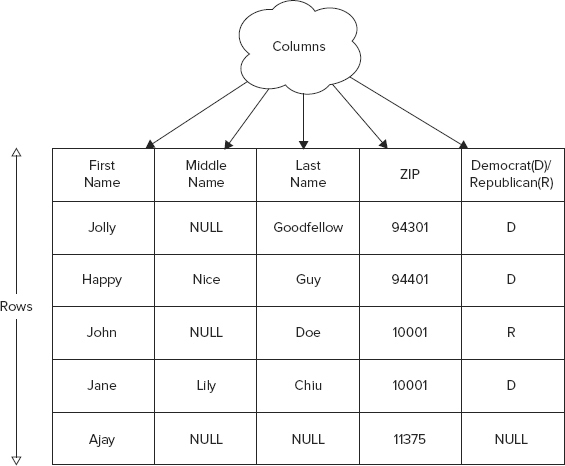
This elementary example has five columns. When you store this table in an RDBMS, you define the data type for each column. For example, you would set the column that stores the first name to VARCHAR, or variable character type, and ZIP to integer (in the United States all ZIP codes are integers). You can have some cells, intersections of rows and columns, with nonexistent values (that is, NULL). For example, Jolly Goodfellow has no middle name and so the middle name column value for this person is NULL.

Typically, an RDBMS table has a few columns, sometimes tens of them. The table itself would hold at most a few thousand records. In special cases, millions of rows could potentially be held in a relational table but keeping such large amounts of data may bring the data access to a halt, unless special considerations like denormalization are applied.

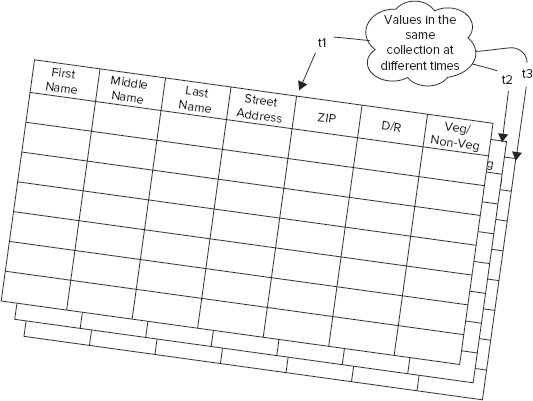
As you begin to use your table to store and access data, you may need to alter it to hold a few additional attributes. Such attributes could be street address and food preferences. As newer records are stored, with values for these newer attributes, you may have null values for these attributes in the existing records. Also, as you keep greater variety of attributes the likelihood of sparse data sets — sets with null in many cells — becomes increasingly real. At some point, your table may look like the one in Figure 4-2.

FIGURE 4-2

Now, consider that this data is evolving and you have to store each version of the cell value as it evolves. Think of it like a three-dimensional Excel spreadsheet, where the third dimension is time. Then the values as they evolve through time could be thought of as cell values in multiple spreadsheets put one behind the other in chronological order. Browse Figure 4-3 to wrap your head around the 3-D Excel spreadsheet abstraction.

FIGURE 4-3

Although the example is extremely simple, you may have sensed that altering the table as data evolves, storing a lot of sparse cells, and working through value versions can get complex. Or more accurately, complex if dealt with the help of RDBMS! You have most likely experienced some of this in your own application.

Contrasting Column Databases with RDBMS

Next, column databases are introduced to model and store the same example. Because the example has been presented using RDBMS so far, understanding column databases in contrast to RDBMS clearly highlights its key features.

First and foremost, a column-oriented database imposes minimal need for upfront schema definition and can easily accommodate newer columns as the data evolves. In a typical column-oriented store, you predefine a column-family and not a column. A column-family is a set of columns grouped together into a bundle. Columns in a column-family are logically related to each other, although this not a requirement. Column-family members are physically stored together and typically a user benefits by clubbing together columns with similar access characteristics into the same family. Few if any theoretical limitations exist on the number of column-families you can define, but keeping them to a minimum can help keep the schema malleable. In the example at hand, defining three column-families, specifically name, location, and preferences, could be enough.

In a column database, a column-family is analogous to a column in an RDBMS. Both are typically defined before data is stored in tables and are fairly static in nature. Columns in RDBMS define the type of data they can store. Column-families have no such limitation; they can contain any number of columns, which can store any type of data, as far as they can be persisted as an array of bytes.

Each row of a column-oriented database table stores data values in only those columns for which it has valid values. Null values are not stored at all. At this stage, you may benefit from seeing Figure 4-4, where the current example is morphed to fit a column store model.

FIGURE 4-4

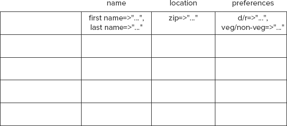
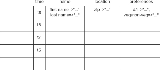
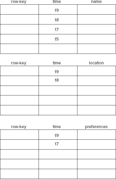
Apart from being friendly storage containers for sparse and malleable data sets, column databases also store multiple versions of each cell. Therefore, continuously evolving data in the current example would get stored in a column database as shown in Figure 4-5.

FIGURE 4-5

On physical stores, data isn’t stored as a single table but is stored by column-families. Column databases are designed to scale and can easily accommodate millions of columns and billions of rows. Therefore, a single table often spans multiple machines. A row-key uniquely identifies a row in a column database. Rows are ordered and split into bundles, containing contiguous values, as data grows. Figure 4-6 is a closer depiction of how data is stored physically.

FIGURE 4-6

A typical column database is deployed in a cluster, although you can run it in a single node for development and experimental purposes. Each column database has its own idiosyncratic network topology and deployment architecture, but learning about any one of them in depth should provide a typical scenario.

The HBase architecture is explained in a section titled, “HBase Distributed Storage Architecture,” later in this chapter. In that section you learn more about a typical deployment layout.

Column Databases as Nested Maps of Key/Value Pairs

Although thinking of column databases as tables with special properties is easy to understand, it creates confusion. Often terms like columns and tables immediately conjure ideas of relational databases and lead you to planning the schema as such. This can be detrimental and often causes developers to relapse into using column databases like relational stores. That is certainly one design pitfall everyone needs to avoid. Always remember that using the right tool for the job is more important than the tool itself. If RDBMS is what you need, then just use it. However, if you are using a column database to scale out your huge data store, then work with it without any RDBMS baggage.

Oftentimes, it’s easier to think of column databases as a set of nested maps. Maps or hash maps, which are also referred to as associative arrays, are pairs of keys and their corresponding values. Keys need to be unique to avoid collision and values can often be any array of bytes. Some maps can hold only string keys and values but most column databases don’t have such a restriction.

It’s not surprising that Google Bigtable, the original inspiration for current-generation column databases, is officially defined as a sparse, distributed, persistent, multidimensional, and sorted map.

“Bigtable: A Distributed Storage System for Structured Data,” Fay Chang, et al. OSDI 2006, http://labs.google.com/papers/bigtable-osdi06.pdf in section 2, titled Data Model, defines Bigtable like so:

“A Bigtable is a sparse, distributed, persistent multi-dimensional sorted map. The map is indexed by a row-key, column key, and a timestamp; each value in the map is an un-interpreted array of bytes.”

Viewing the running example as a multidimensional nested map, you could create the first two levels of keys in JSON-like representation, like so:

{
  "row_key_1" : {
    "name" : {
    ...
    },
    "location" : {
    ...
    },
    "preferences" : {
    ...
    }
  },
  "row_key_2" : {
    "name" : {
    ...
    },
    "location" : {
    ...
    },
    "preferences" : {
    ...
    }
  },
  "row_key_3" : {
  ...
}

The first-level key is the row-key that uniquely identifies a record in a column database. The second-level key is the column-family identifier. Three column-families — name, location, and preferences — were defined earlier. Those three appear as second-level keys. Going by the pattern, you may have guessed that the third-level key is the column identifier. Each row may have a different set of columns within a column-family, so the keys at level three may vary between any two data points in the multidimensional map. Adding the third level, the map is like so:

{
  "row_key_1" : {
    "name" : {
      "first_name" : "Jolly",
      "last_name" : "Goodfellow"
      }
      
      }
    },
    "location" : {
      "zip": "94301"
    },
    "preferences" : {
      "d/r" : "D"
    }
  },
  "row_key_2" : {
    "name" : {
      "first_name" : "Very",
      "middle_name" : "Happy",
      "last_name" : "Guy"
    },
    "location" : {
      "zip" : "10001"
    },
    "preferences" : {
      "v/nv": "V"
    }
  },
  ...
}

Finally, adding the version element to it, the third level can be expanded to include timestamped versions. To show this, the example uses arbitrary integers to represent timestamp-driven versions and concocts a tale that Jolly Goodfellow declared his democratic inclinations at time 1 and changed his political affiliation to the Republicans at time 5. The map for this row then appears like so:

{
  "row_key_1" : {
    "name" : {
      "first_name" : {
        1 : "Jolly"
       },
      "last_name" : {
        1 : "Goodfellow"
      }
    },
    "location" : {
      "zip": {
        1 : "94301"
      }
    },
    "preferences" : {
      "d/r" : {
        1 : "D",
        5 : "R"
      }
    }
  },
  ...
}

That limns a map-oriented picture of a column-oriented database. If the example isn’t detailed enough for you, consider reading Jim Wilson’s write-up titled, “Understanding HBase and Bigtable,” accessible online at http://jimbojw.com/wiki/index.php?title=Understanding_Hbase_and_BigTable.

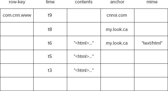
Laying out the Webtable

No discussion of column databases is complete without the quintessential example of a so-called Webtable that stores copies of crawled web pages. Such a table stores the contents of a web page in addition to attributes that relate to the page. Such attributes can be an anchor that references the page or the mime types that relate to the content. Google first introduced this example in its research paper on Bigtable. A Webtable uses a reversed web page URL as the row-key for a web page. Therefore, a URL www.example.com implies a row-key com.example.www. The row-key forms the premise of order for rows of data in a column-oriented database. Therefore, rows that relate to two subdomains of example.com, like www.example.com and news.example.com, are stored close to each other when reversed URL is used as a row-key. This makes querying for all content relating to a domain easier.

Typically, contents, anchors, and mime serve as column-families, which leads to a conceptual model that resembles the column-based table shown Figure 4-7.

FIGURE 4-7

Many popular open-source implementations of Bigtable include the Webtable as an example in their documentation. The HBase architecture wiki entry, at http://wiki.apache.org/hadoop/Hbase/HbaseArchitecture, talks about Webtable and so does the Hypertable data model documentation at http://code.google.com/p/hypertable/wiki/ArchitecturalOverview#Data_Model.

Now that you have a conceptual overview of column databases, it’s time to peek under the hood of a prescribed HBase deployment and storage model. The distributed HBase deployment model is typical of many column-oriented databases and serves as a good starting point for understanding web scale database architecture.

HBASE DISTRIBUTED STORAGE ARCHITECTURE

A robust HBase architecture involves a few more parts than HBase alone. At the very least, an underlying distributed, centralized service for configuration and synchronization is involved. Figure 4-8 depicts an overview of the architecture.

FIGURE 4-8

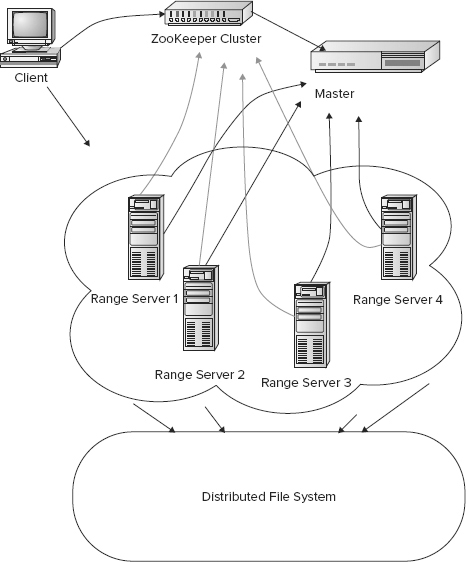
HBase deployment adheres to a master-worker pattern. Therefore, there is usually a master and a set of workers, commonly known as range servers. When HBase starts, the master allocates a set of ranges to a range server. Each range stores an ordered set of rows, where each row is identified by a unique row-key. As the number of rows stored in a range grows in size beyond a configured threshold, the range is split into two and rows are divided between the two new ranges.

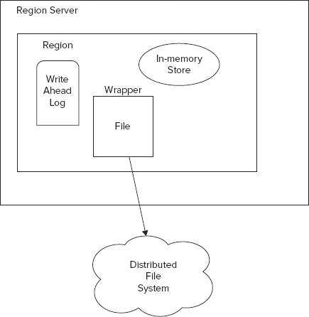
Like most column-databases, HBase stores columns in a column-family together. Therefore, each region maintains a separate store for each column-family in every table. Each store in turn maps to a physical file that is stored in the underlying distributed filesystem. For each store, HBase abstracts access to the underlying filesystem with the help of a thin wrapper that acts as the intermediary between the store and the underlying physical file.

Each region has an in-memory store, or cache, and a write-ahead-log (WAL). To quote Wikipedia, http://en.wikipedia.org/wiki/Write-ahead_logging, “write-ahead logging (WAL) is a family of techniques for providing atomicity and durability (two of the ACID properties) in database systems.” WAL is a common technique used across a variety of database systems, including the popular relational database systems like PostgreSQL and MySQL. In HBase a client program could decide to turn WAL on or switch it off. Switching it off would boost performance but reduce reliability and recovery, in case of failure. When data is written to a region, it’s first written to the write-ahead-log, if enabled. Soon afterwards, it’s written to the region’s in-memory store. If the in-memory store is full, data is flushed to disk and persisted in the underlying distributed storage. See Figure 4-9, which recaps the core aspects of a region server and a region.

FIGURE 4-9

If a distributed filesystem like the Hadoop distributed filesystem (HDFS) is used, then a master-worker pattern extends to the underlying storage scheme as well. In HDFS, a namenode and a set of datanodes form a structure analogous to the configuration of master and range servers that column databases like HBase follow. Thus, in such a situation each physical storage file for an HBase column-family store ends up residing in an HDFS datanode. HBase leverages a filesystem API to avoid strong coupling with HDFS and so this API acts as the intermediary for conversations between an HBase store and a corresponding HDFS file. The API allows HBase to work seamlessly with other types of filesystems as well. For example, HBase could be used with CloudStore, formerly known as Kosmos FileSystem (KFS), instead of HDFS.

Read more about CloudStore, formerly known as Kosmos FileSystem (KFS), at http://kosmosfs.sourceforge.net/.

In addition to having the distributed filesystem for storage, an HBase cluster also leverages an external configuration and coordination utility. In the seminal paper on Bigtable, Google named this configuration program Chubby. Hadoop, being a Google infrastructure clone, created an exact counterpart and called it ZooKeeper. Hypertable calls the similar infrastructure piece Hyperspace. A ZooKeeper cluster typically front-ends an HBase cluster for new clients and manages configuration.

To access HBase the first time, a client accesses two catalogs via ZooKeeper. These catalogs are named -ROOT- and .META. The catalogs maintain state and location information for all the regions. -ROOT- keeps information of all .META. tables and a .META. file keeps records for a user-space table, that is, the table that holds the data. When a client wants to access a specific row it first asks ZooKeeper for the -ROOT- catalog. The -ROOT- catalog locates the .META. catalog relevant for the row, which in turn provides all the region details for accessing the specific row. Using this information the row is accessed. The three-step process of accessing a row is not repeated the next time the client asks for the row data. Column databases rely heavily on caching all relevant information, from this three-step lookup process. This means clients directly contact the region servers the next time they need the row data. The long loop of lookups is repeated only if the region information in the cache is stale or the region is disabled and inaccessible.

Each region is often identified by the smallest row-key it stores, so looking up a row is usually as easy as verifying that the specific row-key is greater than or equal to the region identifier.

So far, the essential conceptual and physical models of column database storage have been introduced. The behind-the-scenes mechanics of data write and read into these stores have also been exposed. Advanced features and detailed nuances of column databases will be picked up again in the later chapters, but for now I shift focus to document stores.

DOCUMENT STORE INTERNALS

The previous couple of chapters have offered a user’s view into a popular document store MongoDB. Now take the next step to peel the onion’s skin.

MongoDB is a document store, where documents are grouped together into collections. Collections can be conceptually thought of as relational tables. However, collections don’t impose the strict schema constraints that relational tables do. Arbitrary documents could be grouped together in a single collection. Documents in a collection should be similar, though, to facilitate effective indexing. Collections can be segregated using namespaces but down in the guts the representation isn’t hierarchical.

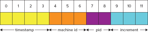
Each document is stored in BSON format. BSON is a binary-encoded representation of a JSON-type document format where the structure is close to a nested set of key/value pairs. BSON is a superset of JSON and supports additional types like regular expression, binary data, and date. Each document has a unique identifier, which MongoDB can generate, if it is not explicitly specified when the data is inserted into a collection, like when auto-generated object ids are, as depicted in Figure 4-10.

FIGURE 4-10

MongoDB drivers and clients serialize and de-serialize to and from BSON as they access BSON-encoded data. The MongoDB server, on the other hand, understands the BSON format and doesn’t need the additional overhead of serialization. The binary representations are read in the same format as they are transferred across the wire. This provides a great performance boost.

High performance is an important philosophy that pervades much of MongoDB design. One such choice is demonstrated in the use of memory-mapped files for storage.

Storing Data in Memory-Mapped Files

A memory-mapped file is a segment of virtual memory that is assigned byte-for-byte to a file or a file-like resource that can be referenced through a file descriptor. This implies that applications can interact with such files as if they were parts of the primary memory. This obviously improves I/O performance as compared to usual disk read and write. Accessing and manipulating memory is much faster than making system calls. In addition, in many operating systems, like Linux, memory region mapped to a file is part of the buffer of disk-backed pages in RAM. This transparent buffer is commonly called page cache. It is implemented in the operating system’s kernel.

MongoDB’s strategy of using memory-mapped files for storage is a clever one but it has its ramifications. First, memory-mapped files imply that there is no separation between the operating system cache and the database cache. This means there is no cache redundancy either. Second, caching is controlled by the operating system, because virtual memory mapping does not work the same on all operating systems. This means cache-management policies that govern what is kept in cache and what is discarded also varies from one operating system to the other. Third, MongoDB can expand its database cache to use all available memory without any additional configuration. This means you could enhance MongoDB performance by throwing in a larger RAM and allocating a larger virtual memory.

Memory mapping also introduces a few limitations. For example, MongoDB’s implementation restricts data size to a maximum of 2 GB on 32-bit systems. These restrictions don’t apply to MongoDB running on 64-bit machines.

Database size isn’t the only size limitation, though. Additional limitations govern the size of each document and the number of collections a MongoDB server can hold. A document can be no larger than 8 MiB, which obviously means using MongoDB to store large blobs is not appropriate. If storing large documents is absolutely necessary, then leverage the GridFS to store documents larger than 8 MiB. Furthermore, there is a limit on the number of namespaces that can be assigned in a database instance. The default number of namespaces supported is 24,000. Each collection and each index uses up a namespace. This means, by default, two indexes per collection would allow a maximum of 8,000 collections per database. Usually, such a large number is enough. However, if you need to, you can raise the namespace size beyond 24,000.

Increasing the namespace size has implications and limitations as well. Each collection namespace uses up a few kilobytes. In MongoDB, an index is implemented as a B-tree. Each B-tree page is 8 kB. Therefore, adding additional namespaces, whether for collections or indexes, implies adding a few kB for each additional instance. Namespaces for a MongoDB database named mydb are maintained in a file named mydb.ns. An .ns file like mydb.ns can grow up to a maximum size of 2 GB.

Because size limitations can restrict unbounded database growth, it’s important to understand a few more behavioral patterns of collections and indexes.

Guidelines for Using Collections and Indexes in MongoDB

Although there is no formula to determine the optimal number of collections in a database, it’s advisable to stay away from putting a lot of disparate data into a single collection. Mixing an eclectic bunch together creates complexities for indexes. A good rule of thumb is to ask yourself whether you often need to query across the varied data set. If your answer is yes you should keep the data together, otherwise portioning it into separate collections is more efficient.

Sometimes, a collection may grow indefinitely and threaten to hit the 2 GB database size limit. Then it may be worthwhile to use capped collections. Capped collections in MongoDB are like a stack that has a predefined size. When a capped collection hits its limit, old data records are deleted. Old records are identified on the basis of the Least Recently Used (LRU) algorithm. Document fetching in capped collection follows a Last-In-First-Out (LIFO) strategy.

Read more about the Least Recently Used (LRU) caching algorithm at http://en.wikipedia.org/wiki/Cache_algorithms#Least_Recently_Used.

Its _id field indexes every MongoDB collection. Additionally, indexes can be defined on any other attributes of the document. When queried, documents in a collection are returned in natural order of their _id in the collection. Only capped collections use a LIFO-based order, that is, insertion order. Cursors return applicable data in batches, each restricted by a maximum size of 8 MiB. Updates to records are in-place.

MongoDB offers enhanced performance but it does so at the expense of reliability.

MongoDB Reliability and Durability

First and foremost, MongoDB does not always respect atomicity and does not define transactional integrity or isolation levels during concurrent operations. So it’s possible for processes to step on each other’s toes while updating a collection. Only a certain class of operations, called modifier operations, offers atomic consistency.

MongoDB defines a few modifier operations for atomic updates:

• $inc — Increments the value of a given field
• $set — Sets the value for a field
• $unset — Deletes the field
• $push — Appends value to a field
• $pushAll — Appends each value in an array to a field
• $addToSet — Adds value to an array if it isn’t there already
• $pop — Removes the last element in an array
• $pull — Removes all occurrences of values from a field
• $pullAll — Removes all occurrences of each value in an array from a field
• $rename — Renames a field

The lack of isolation levels also sometimes leads to phantom reads. Cursors don’t automatically get refreshed if the underlying data is modified.

By default, MongoDB flushes to disk once every minute. That’s when the data inserts and updates are recorded on disk. Any failure between two synchronizations can lead to inconsistency. You can increase the sync frequency or force a flush to disk but all of that comes at the expense of some performance.

To avoid complete loss during a system failure, it’s advisable to set up replication. Two MongoDB instances can be set up in a master-slave arrangement to replicate and keep the data in synch. Replication is an asynchronous process so changes aren’t propagated as soon as they occur. However, it’s better to have data replicated than not have any alternative at all. In the current versions of MongoDB, replica pairs of master and slave have been replaced with replica sets, where three replicas are in a set. One of the three assumes the role of master and the other two act as slaves. Replica sets allow automatic recovery and automatic failover.

Whereas replication is viewed more as a failover and disaster recovery plan, sharding could be leveraged for horizontal scaling.

Horizontal Scaling

One common reason for using MongoDB is its schema-less collections and the other is its inherent capacity to perform well and scale. In more recent versions, MongoDB supports auto-sharding for scaling horizontally with ease.

The fundamental concept of sharding is fairly similar to the idea of the column database’s master-worker pattern where data is distributed across multiple range servers. MongoDB allows ordered collections to be saved across multiple machines. Each machine that saves part of the collection is then a shard. Shards are replicated to allow failover. So, a large collection could be split into four shards and each shard in turn may be replicated three times. This would create 12 units of a MongoDB server. The two additional copies of each shard serve as failover units.

Shards are at the collection level and not at the database level. Thus, one collection in a database may reside on a single node, whereas another in the same database may be sharded out to multiple nodes.

Each shard stores contiguous sets of the ordered documents. Such bundles are called chunks in MongoDB jargon. Each chunk is identified by three attributes, namely the first document key (min key), the last document key (max key), and the collection.

A collection can be sharded based on any valid shard key pattern. Any document field of a collection or a combination of two or more document fields in a collection can be used as the basis of a shard key. Shard keys also contain an order direction property in addition to the field to define a shard key. The order direction can be 1, meaning ascending or –1, meaning descending. It’s important to choose the shard keys prudently and make sure those keys can partition the data in an evenly balanced manner.

All definitions about the shards and the chunks they maintain are kept in metadata catalogs in a config server. Like the shards themselves, config servers are also replicated to support failover.

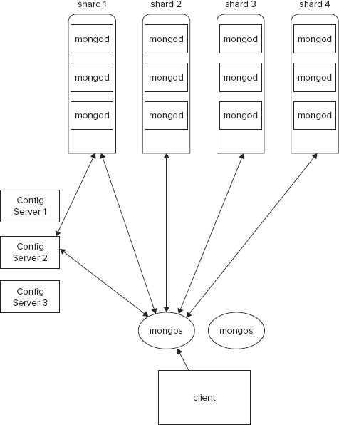
Client processes reach out to a MongoDB cluster via a mongos process. A mongos process does not have a persistent state and pulls state from the config servers. There can be one or more mongos processes for a MongoDB cluster. Mongos processes have the responsibility of routing queries appropriately and combining results where required. A query to a MongoDB cluster can be targeted or can be global. All queries that can leverage the shard key on which the data is ordered typically are targeted queries and those that can’t leverage the index are global. Targeted queries are more efficient than global queries. Think of global queries as those involving full collection scans.

Figure 4-11 depicts a sharding architecture topology for MongoDB.

FIGURE 4-11

Next, I survey the storage schemes and nuances of a key/value store.

UNDERSTANDING KEY/VALUE STORES IN MEMCACHED AND REDIS

Though all key/value stores are not the same, they do have many things in common. For example, they all store data as maps. In this section I walk through the internals of Memcached and Redis to show what a robust key/value store is made up of.

Under the Hood of Memcached

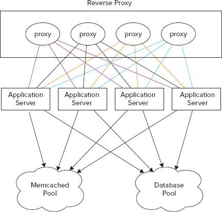
Memcached, which you can download from http://memcached.org, is a distributed high-performance object-caching system. It’s extremely popular and used by a number of high-traffic venues like Facebook, Twitter, Wikipedia, and YouTube. Memcached is extremely simple and has a bare minimum set of features. For example, there is no support for backup, failover, or recovery. It has a simple API and can be used with almost any web-programming language. The primary objective of using Memcached in an application stack is often to reduce database load. See Figure 4-12 to understand a possible configuration for Memcached in a typical web application.

FIGURE 4-12

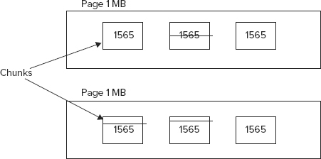
The heart of Memcached is a slab allocator. Memcached stores its values in a slab. A slab itself is composed of pages, which in turn are made up of chunks or buckets. The smallest size a slab can be is 1 kB and slab sizes grow at a power of 1.25. Therefore, slab sizes can be 1 kB (1.25 power 0), 1.25 kB (1.25 power 1), 1.5625 kB (1.25 power 2), and so on. Memcached can store data values up to a maximum of 1 MB in size. Values are stored and referenced by a key. A key can be up to 250 bytes in size. Each object is stored in a closest sized chunk or bucket. This means an object 1.4 kB in size would be stored in a chuck that is 1.5625 kB in size. This leads to wasted space, especially when objects are barely larger than the next smaller chunk size. By default, Memcached uses up all available memory and is limited only by the underlying architecture. Figure 4-13 illustrates some of the fundamental Memcached characteristics.

FIGURE 4-13

LRU algorithms govern the eviction of old cache objects. LRU algorithms work on a per-slab class basis. Fragmentation may occur as objects are stored and cleaned up. Reallocation of memory solves part of this problem.

Memcached is an object cache that doesn’t organize data elements in collections, like lists, sets, sorted sets, or maps. Redis, on the other hand, provides support for all these rich data structures. Redis is similar to Memcached in approach but more robust. You have set up and interacted with Redis in the last couple of chapters.

Next, the innards of Redis are briefly explored.

Redis Internals

Everything in Redis is ultimately represented as a string. Even collections like lists, sets, sorted sets, and maps are composed of strings. Redis defines a special structure, which it calls simple dynamic string or SDS. This structure consists of three parts, namely:

• buff — A character array that stores the string
• len — A long type that stores the length of the buff array
• free — Number of additional bytes available for use

Although you may think of storing len separately as an overhead, because it can be easily calculated based on the buff array, it allows for string length lookup in fixed time.

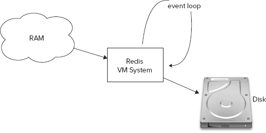
Redis keeps its data set in the primary memory, persisting it to disk as required. Unlike MongoDB, it does not use memory-mapped files for that purpose. Instead, Redis implements its own virtual memory subsystem. When a value is swapped to disk, a pointer to that disk page is stored with the key. Read more about the virtual memory technical specification at http://code.google.com/p/redis/wiki/VirtualMemorySpecification.

In addition to the virtual memory manager, Redis also includes an event library that helps coordinate the non-blocking socket operations.

Figure 4-14 depicts an overview of the Redis architecture.

FIGURE 4-14

Next and last of all, attention is diverted back to column-oriented databases. However, this time it’s a special class of column-oriented databases, those that are eventually consistent.

EVENTUALLY CONSISTENT NON-RELATIONAL DATABASES

Whereas Google’s Bigtable serves as the inspiration for column databases, Amazon’s Dynamo acts as the prototype for an eventually consistent store. The ideas behind Amazon Dynamo were presented in 2007 at the Symposium on Operating Systems Principles and were made available to the public via a technical paper, which is available online at www.allthingsdistributed.com/files/amazon-dynamo-sosp2007.pdf. In due course, the ideas of Dynamo where incorporated into open-source implementations like Apache Cassandra, Voldemort, Riak, and Dynomite. In this section the fundamental tenets of an eventually consistent key/value store are discussed. Specifics of any of the open-source implementations are left for later chapters.

Amazon Dynamo powers a lot of the internal Amazon services that drive its massive e-commerce system. This system has a few essential requirements like high availability and fault tolerance. However, data sets are structured such that query by primary keys is enough for most cases. Relational references and joins are not required. Dynamo is built on the ideas of consistent hashing, object versioning, gossip-based membership protocol, merkle trees, and hinted handoff.

Dynamo supports simple get-and-put-based interface to the data store. Put requests include data related to object version, which are stored in the context. Dynamo is built to incrementally scale as the data grows. Thus, it relies on consistent hashing for effective partitioning.

Consistent Hashing

Consistent hashing forms an important principle for distributed hash tables. In consistent hashing, addition or removal of a slot does not significantly change the mapping of keys to the slots. To appreciate this hashing scheme, let’s first look at an elementary hashing scheme and understand the problems that show up as slots are added or removed.

A very rudimentary key allocation strategy among a set of nodes could involve the use of modulo function. So, 50 keys can be distributed among 7 nodes like so: key with value 85 goes to node 1 because 85 modulo 7 is 1 and key with value 18 goes to node 4 because 18 modulo 7 is 4, and so on for others. This strategy works well until the number of nodes changes, that is, newer ones get added or existing ones get removed. When the number of nodes changes, the modulo function applied to the existing keys produces a different output and leads to rearrangement of the keys among the nodes. This isn’t that effective and that’s when consistent hashing comes to the rescue.

In consistent hashing, the rearrangement of keys is not majorly affected when nodes are added or removed. A good way to explain consistent hashing is to draw out a circle and mark the nodes on it as shown in Figure 4-15.

FIGURE 4-15

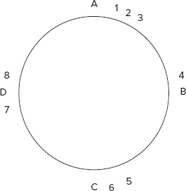
Now the keys themselves are assigned to the nodes that they are closest to. Which means in Figure 4-15, 1, 2, 3 get assigned to node A, 4 gets assigned to B, 5 and 6 get assigned to C, and 7 and 8 to D. In order to set up such a scheme, you may create a large hash space, say all the SHA1 keys up to a very large number, and map that onto a circle. Starting from 0 and going clockwise, you would map all values to a maximum, at which point you would restart at 0. The nodes would also be hashed and mapped on the same scheme.

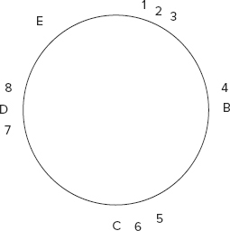
Now say node A is removed and instead node E gets added at a new position as shown in Figure 4-16, then minimum rearrangement occurs. 1 goes to E and 2 and 3 get allocated to B but nothing else gets affected.

FIGURE 4-16

Whereas consistent hashing provides effective partitioning, object versioning helps keep the data consistent.

Object Versioning

In a large distributed and highly scalable system, ACID transactions impose a huge overhead. So Dynamo proposes object versioning and vector clocks for keeping consistency. Let’s try to understand how a vector clock works with the help of an example.

Let’s consider that four hackers, Joe, Hillary, Eric, and Ajay, decide to meet to talk about vector clocks. Joe suggests they all meet up in Palo Alto. Then later, Hillary and Eric meet at work and decide that Mountain View may be the best place for the meeting. The same day, Eric and Ajay message each other and conclude that meeting at Los Altos may be the best idea. When the day of the meeting arrives, Joe e-mails everyone with a meet-up reminder and the venue address in Palo Alto. Hillary responds that the venue was changed to Mountain View and Ajay says it’s Los Altos. Both claim that Eric knows of the decision. Now Eric is contacted to resolve the issue. At this stage you can create vector clocks to resolve the conflict.

A vector clock can be created for each of the three values for the venue, Palo Alto, Mountain View, and Los Altos, as follows:

Venue: Palo Alto
Vector Clock: Joe (ver 1)

Venue: Mountain View
Vector Clock: Joe (ver 1), Hillary (ver 1), Eric (ver 1)

Venue: Los Altos
Vector Clock: Joe (ver 1), Ajay (ver 1), Eric (ver 1)

The vector clocks for Mountain View and Los Altos include Joe’s original choice because everyone was aware of it. The vector clock for Mountain View is based on Hillary’s response, and the vector clock for Los Altos is based on Ajay’s response. The Mountain View and Los Altos vector clocks are out of sync, because they don’t descend from each other. A vector clock needs to have versions greater than or equal to all values in another vector clock to descend from it.

Finally, Joe gets hold of Eric on the phone and asks him to resolve the confusion. Eric realizes the problem and quickly decides that meeting in Mountain View is probably the best idea. Now Joe draws out the updated vector clocks as follows:

Venue: Palo Alto
Vector Clock: Joe (ver 1)

Venue: Mountain View
Vector Clock: Joe (ver 1), Hillary (ver 1), Ajay (ver 0), Eric (ver 2)

Venue: Los Altos
Vector Clock: Joe (ver 1), Hillary (ver 0), Ajay (ver 1), Eric (ver 1)

Version 0 is created for Hillary and Ajay in the vector clocks for the venues they had not suggested but are now aware of. Now, vector clocks descend from each other and Mountain View is the venue for the meet up. From the example, you would have observed that vector clocks not only help determine the order of the events but also help resolve any inconsistencies by identifying the root causes for those problems.

Apart from object versioning, Dynamo uses gossip-based membership for the nodes and uses hinted handoff for consistency.

Gossip-Based Membership and Hinted Handoff

A gossip protocol is a style of communication protocol inspired by the form of gossip or rumor in social networks and offices. A gossip communication protocol involves periodic, pair wise, inter-process interactions. Reliability is usually low and peer selection is often random.

In hinted handoff, instead of a full quorum during message write for durability, a relaxed quorum is allowed. Write is performed on the healthy nodes and hints are recorded to let the failed node know when it’s up again.

SUMMARY

This chapter was a brief introduction to the basic principles of NoSQL databases. The essentials of data models, storage schemes, and configuration in some of the popular NoSQL stores were explained. Typical parts of column-oriented databases were presented and examples from HBase were used to illustrate some of the common underlying themes. Then the internals of both document databases and key/value stores were covered. Finally, eventually consistent databases were introduced.