Chapter 5

Performing CRUD Operations

WHAT’S IN THIS CHAPTER?

• Describing create, read, update, and delete operations as they relate to data sets in a NoSQL database
• Explaining and illustrating the emphasis on create over update
• Exploring the atomicity and integrity of updates
• Explaining the ways of persisting related data

The set of essential operations — create, read, update, and delete, often popularly known as CRUD — are the fundamental ways of interacting with any data. So it’s important to see how these operations apply to the world of NoSQL. As you know, NoSQL isn’t a single product or technology, but an umbrella term for a category of databases; therefore, the implication of CRUD operations varies from one NoSQL product to the other. However, there is one predominant characteristic they all share: in NoSQL stores, the create and read operations are more important than the update and delete operations, so much so that sometimes those are the only operations. In the next few sections you learn what this implies. As the land of NoSQL is explored from the standpoint of the CRUD operations, it will be divided into subsets of column-oriented, document-centric, and key-value maps to keep the illustration within logical and related units.

The first pillar of CRUD is the create operation.

CREATING RECORDS

The record-creation operation hardly needs a definition. When you need a new record to be saved for the first time, you create a new entry. This means there should be a way to identify a record easily and find out if it already exists. If it does, you probably want to update the record and not re-create it.

In relational databases, records are stored within a table, where a key, called the primary key, identifies each record uniquely. When you need to check if a record already exists, you retrieve the primary key of the record in question and see if the key exists in the table. What if the record has no value for a primary key, but the values it holds for each of the columns or fields in the table match exactly to the corresponding values of an existing record? This is where things get tricky.

Relational databases uphold the normalization principles introduced by E.F. Codd, a proponent of the relational model. E.F. Codd and Raymond F. Boyce put together a Boyce-Codd Normal Form (BCNF) in 1974 that is often taken as the minimum expected level to keep a database schema normalized. Informally stated, a normalized schema tries to reduce the modification anomalies in record sets by storing data only once and creating references to associated data where necessary. You can read more about database normalization at http://en.wikipedia.org/wiki/Database_normalization and at http://databases.about.com/od/specificproducts/a/normalization.htm.

In a normalized schema, two records with identical values are the same record. So there is an implicit compare-by-value, which is codified in a single column — the primary key — in a relational model. In the world of programming languages, especially object-oriented languages, this notion of identity is often replaced by the compare-by-reference semantics, where a unique record set, existing as an object, is identified uniquely by the memory space it addresses. Because NoSQL encompasses databases that resemble both traditional tabular structures and object stores, the identity semantics vary from value-based to reference-based. In all cases, though, the notion of a unique primary key is important and helps identify a record.

Although a majority of databases allow you to choose an arbitrary string or an array of bytes for a unique record key, they often prescribe a few rules to make sure such a key is unique and meaningful. In some databases, you are assisted with utility functions to generate primary keys.

Now that you understand the record identifier, the following sections cover creating records in a few NoSQL databases. In the previous few chapters, MongoDB, HBase, and Redis were used as examples for document-centric, column-oriented, and key/value maps, respectively. In this section, these three databases are leveraged again.

Creating Records in a Document-Centric Database

A typical example used in many relational database examples is that of a simplified retail system, which creates and manages order records. Each person’s purchase at this fictitious store is an order. An order consists of a bunch of line items. Each order line item includes a product (an item) and number of units of that product purchased. A line item also has a price attribute, which is calculated by multiplying the unit price of the product by the number of units purchased. Each order table has an associated product table that stores the product description and a few other attributes about the product. Figure 5-1 depicts order, product, and their relationship table in a traditional entity-relationship diagram.

FIGURE 5-1

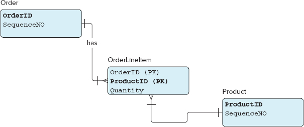
To store this same data in MongoDB, a document store, you would de-normalize the structure and store each order line item detail with the order record itself. As a specific case, consider an order of four coffees: one latte, one cappuccino, and two regular. This coffee order would be stored in MongoDB as a graph of nested JSON-like documents as follows:

{
    order_date: new Date(),
    "line_items": [
        {
            item : {
                name: "latte",
                unit_price: 4.00
            },
            quantity: 1
        },
        {
            item: {
                name: "cappuccino",
                unit_price: 4.25
            },
            quantity: 1
        },
        {
            item: {
                name: "regular",
                unit_price: 2.00
            },
            quantity: 2
        }
    ]
}

coffee_order.txt

Open a command-line window, change to the root of the MongoDB folder, and start the MongoDB server as follows:

bin/mongod --dbpath ~/data/db

Now, in a separate command window, start a command-line client to interact with the server:

bin/mongo

Use the command-line client to store the coffee order in the orders collection, within the mydb database. A partial listing of the command input and response on the console is as follows:

> t = {
...     order_date: new Date(),
...     "line_items": [ ...
...     ]
... };
{
    "order_date" : "Sat Oct 30 2010 22:30:12 GMT-0700 (PDT)",
    "line_items" : [
        {
            "item" : {
                "name" : "latte",
                "unit_price" : 4
            },
            "quantity" : 1
        },
        {
            "item" : {
                "name" : "cappuccino",
                "unit_price" : 4.25
            },
            "quantity" : 1
        },
        {
            "item" : {
                "name" : "regular",
                "unit_price" : 2
            },
            "quantity" : 2
        }
    ]
}
 
> db.orders.save(t);
> db.orders.find();
{ "_id" : ObjectId("4cccff35d3c7ab3d1941b103"), "order_date" : "Sat Oct 30 2010 
22:30:12 GMT-0700 (PDT)", "line_items" : [
    ...
] }

coffee_order.txt

Although storing the entire nested document collection is advised, sometimes it’s necessary to store the nested objects separately. When nested documents are stored separately, it’s your responsibility to join the record sets together. There is no notion of a database join in MongoDB so you must either manually implement the join operation by using the object id on the client side or leverage the concept of DBRef.

In MongoDB DBRef is a formal specification for creating references between documents. A DBRef includes a collection name as well as an object id. Read more about MongoDB DBRef at www.mongodb.org/display/DOCS/Database+References#DatabaseReferences-DBRef.

You can restructure this example in a way that doesn’t store the unit price data for a product in the nested document but keeps it separately in another collection, which stores information on products. In the new format, the item name serves as the key to link between the two collections.

Therefore, the restructured orders data is stored in a collection called orders2 as follows:

> t2 = {
...     order_date: new Date(),
...     "line_items": [
...         {
...             "item_name":"latte",
...             "quantity":1
...         },
...         {
...             "item_name":"cappuccino",
...             "quantity":1
...         },
...         {
...             "item_name":"regular",
...             "quantity":2
...         }
...     ]
... };
{
    "order_date" : "Sat Oct 30 2010 23:03:31 GMT-0700 (PDT)",
    "line_items" : [
        {
            "item_name" : "latte",
            "quantity" : 1
        },
        {
            "item_name" : "cappuccino",
            "quantity" : 1
        },
        {
            "item_name" : "regular",
            "quantity" : 2
        }
    ]
}
> db.orders2.save(t2);

coffee_order.txt

To verify that the data is stored correctly, you can return the contents of the orders2 collection as follows:

> db.orders2.find();
{ "_id" : ObjectId("4ccd06e8d3c7ab3d1941b104"), "order_date" : "Sat Oct 30 2010
 23:03:31 GMT-0700 (PDT)", "line_items" : [
    {
        "item_name" : "latte",
        "quantity" : 1
    },
...
] }

coffee_order.txt

Next, save the product data, wherein item name and unit price are stored, as follows:

> p1 = {
...     "_id": "latte",
...     "unit_price":4
... };
{ "_id" : "latte", "unit_price" : 4 }
> db.products.save(p1);

coffee_order.txt

Again, you can verify the record in the products collection with the help of the find method:

> db.products.find();
{ "_id" : "latte", "unit_price" : 4 }

coffee_order.txt

Now, you could manually link the two collections and retrieve related data sets like this:

> order1 = db.orders2.findOne();
{
    "_id" : ObjectId("4ccd06e8d3c7ab3d1941b104"),
    "order_date" : "Sat Oct 30 2010 23:03:31 GMT-0700 (PDT)",
    "line_items" : [
        {
            "item_name" : "latte",
            "quantity" : 1
        },
        {
            "item_name" : "cappuccino",
            "quantity" : 1
        },
        {
            "item_name" : "regular",
            "quantity" : 2
        }
    ]
}
> db.products.findOne( { _id: order1.line_items[0].item_name } );
{ "_id" : "latte", "unit_price" : 4 }

coffee_order.txt

Alternatively, part of this manual process can be automated with the help of DBRef, which is a more formal specification for relating two document collections in MongoDB. To illustrate DBRef, you rehash the orders example and establish the relationship by first defining the products and then setting up a DBRef to products from within the orders collection.

Add latte, cappuccino, and regular, with their respective unit prices, to the product2 collection as follows:

> p4 = {"name":"latte", "unit_price":4};
{ "name" : "latte", "unit_price" : 4 }
> p5 = {
...     "name": "cappuccino",
...     "unit_price":4.25
... };
{ "_id" : "cappuccino", "unit_price" : 4.25 }
> p6 = {
...     "name": "regular",
...     "unit_price":2
... };
{ "_id" : "regular", "unit_price" : 2 }
> db.products2.save(p4);
> db.products2.save(p5);
> db.products2.save(p6);

coffee_order.txt

Verify that all the three products are in the collection:

> db.products.find();
{ "_id" : ObjectId("4ccd1209d3c7ab3d1941b105"), "name" : "latte", 
  "unit_price" : 4 }
{ "_id" : ObjectId("4ccd1373d3c7ab3d1941b106"), "name" : "cappuccino", 
  "unit_price" : 4.25 }
{ "_id" : ObjectId("4ccd1377d3c7ab3d1941b107"), "name" : "regular", 
  "unit_price" : 2 }

coffee_order.txt

Next, define a new orders collection, called orders3, and use DBRef to establish the relationship between orders3 and products. The orders3 collection can be defined as follows:

t3 = {
...     order_date: new Date(),
...     "line_items": [
...         {
...             "item_name": new DBRef('products2', p4._id),
...             "quantity:1
...         },
...         {
...             "item_name": new DBRef('products2', p5._id),
...             "quantity":1
...         },
...         {
...             "item_name": new DBRef('products2', p6._id),
...             "quantity":2
...         }
...     ]
... };
 
db.orders3.save(t3);

coffee_order.txt

The MongoDB creation process is fairly simple and as you saw, some aspects of the relationship can also be formally established using DBRef. Next, the create operation is viewed in the context of column-oriented databases.

Using the Create Operation in Column-Oriented Databases

Unlike MongoDB databases, column-oriented databases don’t define any concept of relational references. Like all NoSQL products, they avoid joins between collections. So there is no concept of foreign keys or constraints across multiple collections. Column databases store their collections in a de-normalized fashion, almost resembling a data warehouse fact table that keeps large amounts of transactional de-normalized records. Data is stored in such a way that a row-key uniquely identifies each record and that all columns within a column-family are stored together.

Column-oriented databases, in particular HBase, also have a time dimension to save data. Therefore, a create or data insert operation is important but the notion of update is effectively nonexistent. Let’s view these aspects of HBase through an example. Say you had to create and maintain a large catalog of different types of products, where the amounts of information on the type, category, characteristics, price, and source of the product could vary widely. Then you may want to create a table with type, characteristics, and source as three column-families. Individual attributes or fields (also referred to as columns) would then fall within one of these column-families. To create this collection or table of products in HBase, first start the HBase server and then connect to it using the HBase shell. To start the HBase server, open up a command-line window or terminal and change it to the HBase installation directory. Then start the HBase server in local standalone mode as follows:

bin/start-hbase.sh

Open another command-line window and connect to the HBase server using the HBase shell:

bin/hbase shell

Next, create the products table:

hbase(main):001:0> create 'products', 'type', 'characteristics', 'source'
0 row(s) in 1.1570 seconds

products_hbase.txt

Once the table is created, you can save data in it. HBase uses the put keyword to denote a data-creation operation. The word “put” connotes a hash map-like operation for data insertion and because HBase under the hood is like a nested hash map, it’s probably more appropriate than the create keyword.

To create a record with the following fields:

• type:category = "coffee beans"
• type:name = "arabica"
• type:genus = "Coffea"
• characteristics: cultivation_method = "organic"
• characteristics: acidity = "low"
• source: country = "yemen"
• source: terrain = "mountainous"

you can put it into the products table like so:

hbase(main):001:0> put 'products', 'product1', 'type:category', 'coffee beans'
0 row(s) in 0.0710 seconds
hbase(main):002:0> put 'products', 'product1', 'type:name', 'arabica'
0 row(s) in 0.0020 seconds
hbase(main):003:0> put 'products', 'product1', 'type:genus', 'Coffea'
0 row(s) in 0.0050 seconds
hbase(main):004:0> put 'products', 'product1', 
  'characteristics: cultivation_method', 'organic'
0 row(s) in 0.0060 seconds
hbase(main):005:0> put 'products', 'product1', 'characteristics: acidity', 'low'
0 row(s) in 0.0030 seconds
hbase(main):006:0> put 'products', 'product1', 'source: country', 'yemen'
0 row(s) in 0.0050 seconds
hbase(main):007:0> put 'products', 'product1', 'source: terrain', 'mountainous'
0 row(s) in 0.0050 seconds
hbase(main):008:0>

products_hbase.txt

Now you can query for the same record to make sure it’s in the data store. To get the record do the following:

hbase(main):008:0> get 'products', 'product1'
COLUMN                       CELL
characteristics: acidity    timestamp=1288555025970, value=lo
characteristics: cultivatio timestamp=1288554998029, value=organic
n_method
source: country             timestamp=1288555050543, value=yemen
source: terrain             timestamp=1288555088136, value=mountainous
type:category               timestamp=1288554892522, value=coffee beans
type:genus                  timestamp=1288554961942, value=Coffea
type:name                   timestamp=1288554934169, value=Arabica
7 row(s) in 0.0190 seconds

products_hbase.txt

What if you put in a value for "type:category" a second time stored as "beans" instead of its original value of "coffee beans" as follows?

hbase(main):009:0> put 'products', 'product1', 'type:category', 'beans'
0 row(s) in 0.0050 seconds

products_hbase.txt

Now, if you get the record again, the output is as follows:

hbase(main):010:0> get 'products', 'product1'
COLUMN                       CELL
characteristics: acidity    timestamp=1288555025970, value=low
characteristics: cultivatio timestamp=1288554998029, value=organic
n_method
source: country             timestamp=1288555050543, value=yemen
source: terrain             timestamp=1288555088136, value=mountainous
type:category               timestamp=1288555272656, value=beans
type:genus                  timestamp=1288554961942, value=Coffea
type:name                   timestamp=1288554934169, value=Arabica
7 row(s) in 0.0370 seconds

products_hbase.txt

You may notice that the value for type:category is now beans instead of coffee beans. In reality, both values are still stored as different versions of the same field value and only the latest one of these is returned by default. To look at the last four versions of the type:category field, run the following command:

hbase(main):011:0> get 'products', 'product1', { COLUMN => 'type:category', 
  VERSIONS => 4 }
COLUMN                       CELL
type:category               timestamp=1288555272656, value=beans
type:category               timestamp=1288554892522, value=coffee beans

There are only two versions so far, so those are returned.

Now, what if the data is very structured, limited, and relational in nature? It’s possible HBase isn’t the right solution at all then.

HBase flattens the data structure, only creating a hierarchy between a column-family and its constituent columns. In addition, it also stores each cell’s data along a time dimension, so you need to flatten nested data sets when such data is stored in HBase.

Consider the retail order system. In HBase, the retail order data could be stored in a couple of ways:

• Flatten all the data sets and store all fields of an order, including all product data, in a single row.
• For each order, maintain all order line items within a single row. Save the product information in a separate table and save a reference to the product row-key with the order line item information.

Going with the first option of flattening the order data, you could end up making the following choices:

• Create one column-family for regular line items and create another one for additional types of line items like discount or rebate.
• Within a regular line item column-family, you could have columns for item or product name, item or product description, quantity, and price. If you flatten everything, remember to have a different key for each line item or else they will end up getting stored together as versions of the same key/value pair. For example, call the product name column product_name_1 instead of calling all of them product_name.

The next example uses Redis to illustrate creating data in a key/value map.

Using the Create Operation in Key/Value Maps

Redis is a simple, yet powerful, data structure server that lets you store values as a simple key/value pair or as a member of a collection. Each key/value pair can be a standalone map of strings or reside in a collection. A collection could be any of the following types: list, set, sorted set, or hash. A standalone key/value string pair is like a variable that can take string values.

You can create a Redis string key/value map like so:

./redis-cli set akey avalue

You can confirm that the value is created successfully with the help of the get command as follows:

./redis-cli get akey

The response, as expected, is avalue. The set method is the same as the create or the put method. If you invoke the set method again but this time set anothervalue for the key, akey, the original value is replaced with the new one. Try out the following:

./redis-cli set akey anothervalue
./redis-cli get akey

The response, as expected, would be the new value: anothervalue.

The familiar set and get commands for a string can’t be used for Redis collections, though. For example, using lpush and rpush creates and populates a list. A nonexistent list can be created along with its first member as follows:

./redis-cli lpush list_of_books 'MongoDB: The Definitive Guide'

books_list_redis.txt

You can use the range operation to verify and see the first few members of the list — list_of_books — like so:

./redis-cli lrange list_of_books  0 -1
1. "MongoDB: The Definitive Guide"

books_list_redis.txt

The range operation uses the index of the first element, 0, and the index of the last element, -1, to get all elements in the list.

In Redis, when you query a nonexistent list, it returns an empty list and doesn’t throw an exception. You run a range query for a nonexistent list — mylist — like so:

./redis-cli lrange mylist 0 -1

Redis returns a message: empty list or set. You can use lpush much as you use rpush to add a member to mylist like so:

./redis-cli rpush mylist 'a member'

Now, of course mylist isn’t empty and repeating a range query reveals the presence of a member.

Members can be added to a list, either on the left or on the right, and can be popped from either direction as well. This allows you to leverage lists as queues or stacks.

For a set data structure, a member can be added using the SADD operation. Therefore, you can add 'a set member' to aset like so:

./redis-cli sadd aset 'a set member'

The command-line program would respond with an integral value of 1 confirming that it’s added to the set. When you rerun the same SADD command, the member is not added again. You may recall that a set, by definition, holds a value only once and so once present it doesn’t make sense to add it again. You will also notice that the program responds with a 0, which indicates that nothing was added. Like sets, sorted sets store a member only once but they also have a sense of order like a list. You can easily add 'a sset member' to a sorted set, called azset, like so:

./redis-cli zadd azset 1 'a sset member'

The value 1 is the position or score of the sorted set member. You can add another member, 'sset member 2', to this sorted set as follows:

./redis-cli zadd azset 4 'sset member 2'

You could verify that the values are stored by running a range operation, similar to the one you used for a list. The sorted set range command is called zrange and you can ask for a range containing the first five values as follows:

./redis-cli zrange azset 0 4
1. "a sset member"
2. "sset member 2"

What happens when you now add a value at position or score 3 and what happens when you try and add another value to position or score 4, which already has a value?

Adding a value to azset at score 3 like so:

./redis-cli zadd azset 3 'member 3'

and running the zrange query like so:

./redis-cli zrange azset 0 4

reveals:

1. "a sset member"
2. "member 3"
3. "sset member 2"

Adding a value at position or score 3 again, like so:

./redis-cli zadd azset 3 'member 3 again'

and running the zrange query like so:

./redis-cli zrange azset 0 4

reveals that the members have been re-positioned to accommodate the new member, like so:

1. "a sset member"
2. "member 3"
3. "member 3 again"
4. "sset member 2"

Therefore, adding a new member to a sorted set does not replace existing values but instead re-orders the members as required.

Redis also defines the concept of a hash, in which members could be added like so:

./redis-cli hset bank account1 2350
./redis-cli hset bank account2 4300

You can verify the presence of the member using the hget, or its variant hgetall, command:

./redis-cli hgetall bank

To store a complicated nested hash, you could create a hierarchical hash key like so:

./redis-cli hset product:fruits apple 1.35
./redis-cli hset product:fruits banana 2.20

Once data is stored in any of the NoSQL data stores, you need to access and retrieve it. After all, the entire idea of saving data is to retrieve it and use it later.

ACCESSING DATA

You have already seen some of the ways to access data. In an attempt to verify whether records were created, some of the simplest get commands have already been explored. Some of the earlier chapters also demonstrated a few standard query mechanisms.

Next, a few advanced data access methods, syntax, and semantics are explored.

Accessing Documents from MongoDB

MongoDB allows for document queries using syntax and semantics that closely resemble SQL. Ironic as it may be, the similarity to SQL in a NoSQL world makes querying for documents easy and powerful in MongoDB.

You are familiar with the query documents from the previous chapters, so you can dive right in to accessing a few nested MongoDB documents. Once again, you use the orders collection in the database mydb, which was created earlier in this chapter.

Start the MongoDB server and connect to it using the mongo JavaScript shell. Change to the mydb database with the use mydb command. First, get all the documents in the orders collection like so:

db.orders.find()

Now, start filtering the collection. Get all the orders after October 25, 2010, that is, with order_date greater than October 25, 2010. Start by creating a date object. In the JavaScript shell it would be:

var refdate = new Date(2010, 9, 25);

JavaScript dates have months starting at 0 instead of 1, so the number 9 represents October. In Python the same variable creation could be like so:

from datetime import datetime
refdate = datetime(2010, 10, 25)

and in Ruby it would be like so:

require 'date'
refdate = Date.new(2010, 10, 25)

Then, pass refdate in a comparator that compares the order_date field values against refdate. The query is as follows:

db.orders.find({"order_date": {$gt: refdate}});

MongoDB supports a rich variety of comparators, including less than, greater than, less than or equal to, greater than or equal to, equal to, and not equal to. In addition, it supports set inclusion and exclusion logic operators like contained in and not contained in a given set.

The data set is a nested document so it can be beneficial to query on the basis of a value of a nested property. In Mongo, doing that is easy. Traversing through the tree using dot notation could access any nested field. To get all documents from the orders collection where line item name is latte, you write the following query:

db.orders.find({ "line_items.item.name" : "latte" })

The dot notation works whether there are single nested values or a list of them as was the case in the orders collection.

MongoDB expression matching supports regular expressions. Regular expressions can be used in nested documents the same way they are used with top-level fields.

In relational databases, indexes are the smart way of making queries faster. In general, the way that works is simple. Indexes provide an efficient lookup mechanism based on a B-tree-like structure that avoids complete table scans. Because less data is searched through to find the relevant records, the queries are faster and more efficient.

MongoDB supports the notion of indexes to speed up queries. By default, all collections are indexed on the basis of the _id value. In addition to this default index, MongoDB allows you to create secondary indexes. Secondary indexes can be created at the top field level or at the nested field levels. For example, you could create an index on the quantity value of a line item as follows:

db.orders.ensureIndex({ "line_items.quantity" : 1 });

Now, querying for all documents where quantity of a line item is 2 can be fairly fast. Try running the following query:

db.orders.find({ "line_items.quantity" : 2 });

Indexes are stored separate from the table and you may recall from an earlier chapter that they use up a namespace.

MongoDB data access seems fairly simple, rich, and robust. However, this isn’t the case for all NoSQL stores, especially not for column-oriented databases.

Accessing Data from HBase

The easiest and most efficient query to run on HBase is one that is based on the row-key. Row-keys in HBase are ordered and ranges of these contiguous row-keys are stored together. Therefore, looking up a row-key typically means finding the highest order range that has the starting row-key smaller than or equal to the given row-key.

This means that designing the row-key correctly for an application is extremely important. It’s a good idea to relate the row-key semantically to the data contained in the table. In the Google Bigtable research paper, row-keys are made up of inverted domain names so all content related to a specific domain is grouped together. Going by these guidelines, it would be a good idea to model the orders table with row-keys that are a combination of the item or product name, the order date, and possibly category. Depending on how the data is to be most often accessed, the combination sequence of these three fields could vary. So, if orders will be most often accessed in chronological order, you may want to create row-keys like so:

<date> + <timestamp> + <category> + <product>

However, if orders would most often be accessed by the category and product names, then create a row-key like so:

<category> + <product> + <date> + <timestamp>

Although row-keys are important and provide an efficient lookup mechanism for huge amounts of data, there is little built in to support secondary indexes. Any query that doesn’t leverage the row-key leads to table scans, which are both expensive and slow.

Third-party tools like Lucene, the search engine framework, have the ability to help create secondary indexes on HBase tables. Next, you review querying the data structure server, Redis.

Querying Redis

Querying Redis is as elegant and easy as inserting records into it is. Earlier you learned that you could get the value of a specific string by using the get command like so:

./redis-cli get akey

or get a range of list values like so:

./redis-cli lrange list_of_books 0 4

Similarly, you could get members of a set like so:

./redis-cli smembers asset

or members of a sorted set like so:

./redis-cli zrevrange azset  0 4

You also saw that set operations like intersection, union, and difference can also be carried out quite easily using the SINTER, SUNION, and SDIFF commands, respectively.

When you move over from the relational world to the world of NoSQL, it isn’t the data creation or querying that you hear about but it’s the data updates and transactional integrity around it that people talk about the most.

Next, you explore how updating and modifying data is managed in NoSQL databases.

UPDATING AND DELETING DATA

The relational world is deeply rooted in ACID semantics for database integrity and upholds different levels of isolation for data update and modification. NoSQL, on the contrary, does not give extreme importance to ACID transactions and in some cases completely ignores it.

To set the context, you first need to understand what ACID means. ACID is an acronym that stands for atomicity, consistency, isolation, and durability. Informally stated, atomicity means a transaction either happens in totality or rolls back. Consistency means each modification to the database takes it from one consistent state to the other. Inconsistent and unresolved states do not exist. Isolation provides the assurance that some other process cannot modify a piece of data when an operation in progress is using it. Durability implies all committed data can be recovered from any sort of a system failure.

As in the other sections, I go over the different types of NoSQL databases one at a time, starting with MongoDB.

Updating and Modifying Data in MongoDB, HBase, and Redis

Unlike relational databases, the concept of locking doesn’t exist in NoSQL stores. This is a choice by design, not coincidence. Databases like MongoDB are meant to be sharded and scalable. In such a situation, locking across distributed shards can be complex and make the process of data updates very slow.

However, despite the lack of locking, a few tips and tricks could help you in updating data in an atomic manner. First of all, update an entire document and not just a few fields of a document. Preferably use the atomic methods to update the document. Available atomic methods are as follows:

• $set — Set a value
• $inc — Increment a particular value by a given amount
• $push — Append a value to an array
• $pushAll — Append several values to an array
• $pull — Remove a value from an existing array
• $pullAll — Remove several value(s) from an existing array

For example, { $set : { "order_date" : new Date(2010, 10, 01) } } updates the order_date in the orders collection in an atomic manner.

An alternative strategy to using atomic operations is to use the update if current principle. Essentially this involves three steps:

The document or row-level locking and atomicity also applies to HBase.

HBase supports a row-level read-write lock. This means rows are locked when any column in that row is being modified, updated, or created. In HBase terms the distinction between create and update is not clear. Both operations perform similar logic. If the value is not present, it’s inserted or else updated.

Therefore, row-level locking is a great idea, unless a lock is acquired on an empty row and then it’s unavailable until it times out.

Redis has a limited concept of a transaction and an operation can be performed within the confines of such a transaction. Redis MULTI command initiates a transactional unit. Calling EXEC after a MULTI executes all the commands and calling DISCARD rolls back the operations. A simple example of atomic increment of two keys: key1 and key2 could be as follows:

> MULTI
OK
> INCR key1
QUEUED
> INCR key2
QUEUED
> EXEC
1) (integer) 1
2) (integer) 1

Limited Atomicity and Transactional Integrity

Though the specifics of minimal atomic support vary from one database to the other, many of these have quite a few similar characteristics. In this subsection, I cover some of the more pervasive ideas around CAP Theorem and eventual consistency.

CAP Theorem states that two of the following three can be maximized at one time:

• Consistency — Each client has the same view of the data
• Availability — Each client can always read and write
• Partition tolerance — System works well across distributed physical networks

More details on CAP Theorem and its impact on NoSQL are explained in Chapter 9.

One more topic that comes up often is the concept of eventual consistency. This term is sometimes confusing and often not properly understood.

Eventual consistency is a consistency model used in the domain of parallel programming and distributed programming. Eventual consistency could be interpreted in two ways, as follows:

• Given a sufficiently long period of time, over which no updates are sent, one can expect that all updates will, eventually, propagate through the system and all the replicas will be consistent.
• In the presence of continuing updates, an accepted update eventually either reaches a replica or the replica retires from service.

Eventual consistency implies Basically Available, Soft state, Eventual consistency (BASE), as opposed to ACID, which I covered earlier.

SUMMARY

This chapter introduced the essential create, read, update, and delete operations in the context of NoSQL databases. The chapter explored the essential operations in light of three kinds of NoSQL stores, namely, document stores, column-oriented databases, and key/value hash maps. MongoDB represents the document stores, HBase represents the column stores, and Redis represents the key/value hash maps.

During the discussion it became clear that for all the data stores, data creation or insertion is more important than updates. In some cases, updates are limited. Toward the end of the chapter, the topic of updates, transactional integrity, and consistency were also explained.