Chapter 13

Surveying Database Internals

WHAT’S IN THIS CHAPTER?

• Peeking under the hood of MongoDB, Membase, Hypertable, Apache Cassandra, and Berkeley DB
• Exploring the internal architectural elements of a few select NoSQL products
• Understanding the under-the-hood design choices

Learning a product or a tool involves at least three dimensions, namely:

• Understanding its semantics and syntax
• Learning by trying and using it
• Understanding its internals and knowing what is happening under the hood

In the preceding chapters, you were exposed to a considerable amount of syntax, especially in the context of MongoDB, Redis, CouchDB, HBase, and Cassandra. Many of the examples illustrated the syntax and explained the concepts so trying them out would have given you a good hands-on head start to learning the NoSQL products. In some chapters, you had the opportunity to peek under the hood. In this chapter you dive deeper into in-depth discovery by exploring the architecture and the internals of a few select NoSQL products. As with the other chapters, the set of products I chose represents different types of NoSQL products. The products discussed in this chapter made it to the list for various reasons, some of which are as follows:

• MongoDB — MongoDB has been featured in many chapters of this book. The book has already covered a few aspects of MongoDB internals and adding to that information base provides a comprehensive enough coverage of the product.
• Membase — As far as key/value in-memory, with the option to persist to disk data stores go, Redis has been the example of choice so far. Many Redis features and internals have been illustrated through multiple chapters. This chapter steps out of the Redis umbrella to cover a competing product, Membase. Membase has gained popularity because its performance characteristics are notable and adoption of the Memcached protocol makes it a drop-in replacement for Memcached.
• Hypertable — As far as sorted ordered column-family stores go, much has been covered with HBase in mind. Although HBase is a popular Google Bigtable clone, a couple of alternatives are built on the same model. The alternatives are Hypertable and Cloudata. Cloudata is the newest of the open-source options but Hypertable is a well-established player. Hypertable is deployed as a scalable data store for many large Internet applications and services. Hypertable is written in C++ and provides superior performance metrics as compared to HBase. So I cover a few aspects of Hypertable in this chapter.
• Apache Cassandra — Google Bigtable and Amazon Dynamo are the two popular blueprints for architecting large-scale NoSQL stores. Apache Cassandra tries to bring together the ideas from both products. Apache Cassandra has been much talked about and its fast writes have created enough excitement. The chapter covers some bits of what Cassandra is made up of.
• Berkeley DB — Berkeley DB is a powerful key/value store that forms the underlying storage of leading NoSQL products like Amazon Dynamo, LinkedIn, Voldemort, and GenieDB.

The coverage of the topics in this chapter is by no means exhaustive or uniform across products. However, the chapter provides enough information to pique your curiosity to explore the internals further, to unwrap the underlying code of these products, to use these products gainfully, and to possibly contribute to making these products better. In addition, the chapter may also inspire you to explore the internals of other NoSQL products. Some of these other NoSQL products may have been mentioned only in passing in this book. Even others may not even have been mentioned.

MONGODB INTERNALS

Many MongoDB commands and usage patterns have been covered in the book so far. Storage and querying mechanisms have been explored and the topic of replication has been touched upon. A few details about the wire format, BSON, have also been introduced. This section illustrates a few important additional aspects of MongoDB. The illustration builds on top of what you already know.

MongoDB follows client-server architecture, commonly found in traditional RDBMSs. Client-server architecture involves a single server and multiple clients connecting to the server. In a sharded and replicated scenario, multiple servers — instead of only one — form the topology. In a standalone mode or in a clustered and sharded topology, data is transported from client to server and back, and among the nodes.

{ "hello": "world" }

"x16x00x00x00x02hellox00 x06x00x00x00worldx00x00"

{ and }—"x16x00x00x00 and x00
"hello":—x02hellox00
 "world"—x06x00x00x00worldx00

MongoDB Wire Protocol

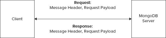
Clients speak to a MongoDB server using a simple TCP/IP-based socket connection. The wire protocol used for the communication is a simple request-response-based socket protocol. The wire protocol headers and payload are BSON encoded. The ordering of messages follows the little endian format, which is the same as in BSON.

In a standard request-response model, a client sends a request to a server and the server responds to the request. In terms of the wire protocol, a request is sent with a message header and a request payload. A response comes back with a message header and a response payload. The format for the message header between the request and the response is quite similar. However, the format of the request and the response payload are not the same. Figure 13-1 depicts the basic request-response communication between a client and a MongoDB server.

FIGURE 13-1

The MongoDB wire protocol allows a number of operations. The allowed operations are as follows:

RESERVED is also an operation, which was formerly used for OP_GET_BY_OID. It’s not listed in the list of opcodes as it’s not actively used.

• OP_INSERT (code: 2002) — Insert a document. The “create” operation in CRUD jargon.
  

  CRUD, which stands for Create, Read, Update and Delete, are standard data management operations. Many systems and interfaces that interact with data facilitate the CRUD operations.

• OP_UPDATE (code: 2001) — Update a document. The update operation in CRUD.
• OP_QUERY (code: 2004) — Query a collection of documents. The “read” operation in CRUD.
• OP_GET_MORE (code: 2005) — Get more data from a query. Query response can contain a large number of documents. To enhance performance and avoid sending the entire set of documents, databases involve the concept of a cursor that allows for incremental fetching of the records. The OP_GET_MORE operation facilitates fetching additional documents via a cursor.
• OP_REPLY (code: 1) — Reply to a client request. This operation sends responses in reply to OP_QUERY and OP_GET_MORE operations.
• OP_KILL_CURSORS (code: 2007) — Operation to close a cursor.
• OP_DELETE (code: 2006) — Delete a document.
• OP_MSG (code: 1000) — Generic message command.

Every request and response message has a header. A standard message header has the following properties:

• messageLength — The length of the message in bytes. Paradoxically, the length includes 4 bytes to hold the length value.
• requestID — A unique message identifier. The client or the server, depending on which is initiating the operation, can generate the identifier.
• responseTo — In the case of OP_QUERY and OP_GET_MORE the response from the database includes the requestID from the original client request as the responseTo value. This allows clients to map requests to responses.
• opCode — The operation code. The allowed operations are listed earlier in this subsection.

Next, you walk through a couple of simple and common request-response scenarios.

Inserting a Document

When creating and inserting a new document, a client sends an OP_INSERT operation via a request that includes:

• A message header — A standard message header structure that includes messageLength, requestID, responseTo, and opCode.
• An int32 value — Zero (which is simply reserved for future use).
• A cstring — The fully qualified collection name. For example, a collection named aCollection in a database named aDatabase will appear as aDatabase.aCollection.
• An array — This array contains one or more documents that need to be inserted into a collection.

The database processes an insert document request and you can query for the outcome of the request by calling the getLastError command. However, the database does not explicitly send a response corresponding to the insert document request.

Querying a Collection

When querying for documents in a collection, a client sends an OP_QUERY operation via a request. It receives a set of relevant documents via a database response that involves an OP_REPLY operation.

An OP_QUERY message from the client includes:

• A message header — A standard header with messageLength, requestID, responseTo, and opCode elements in it.
• An int32 value — Contains flags that represent query options. The flags define properties for a cursor, result streaming, and partial results when some shards are down. For example, you could define whether cursors should close after the last data is returned and you could specify whether idle cursors should be timed out after a certain period of inactivity.
• A cstring — Fully qualified collection name.
• An int32 value — Number of documents to skip.
• Another int32 value — Number of documents to return. A database response with an OP_REPLY operation corresponding to this request receives the documents. If there are more documents than returned, a cursor is also usually returned. The value of this property sometimes varies depending on the driver and its ability to limit result sets.
• A query document in BSON format — Contains elements that must match the documents that are searched.
• A document — Representing the fields to return. This is also in BSON format.

In response to a client OP_QUERY operation request, a MongoDB database server responds with an OP_REPLY. An OP_REPLY message from the server includes:

• A message header — The message header in a client request and a server response is quite similar. Also as mentioned earlier, the responseTo header property for an OP_REPLY would contain the requestID value of the client request for a corresponding OP_QUERY.
• An int32 value — Contains response flags that typically denote an error or exception situation. Response flags could contain information about query failure or invalid cursor id.
• An int64 value — Contains the cursor id that allows a client to fetch more documents.
• An int32 value — Starting point in the cursor.
• Another int32 value — Number of documents returned.
• An array — Contains the documents returned in response to the query.

So far, only a sample of the wire protocol has been presented. You can read more about the wire protocol online at www.mongodb.org/display/DOCS/Mongo+Wire+Protocol. You can also browse through the MongoDB code available at https://github.com/mongodb.

The documents are all stored at the server. Clients interact with the server to insert, read, update, and delete documents. You have seen that the interactions between a client and a server involve an efficient binary format and a wire protocol. Next is a view into the storage scheme.

MongoDB Database Files

MongoDB stores database and collection data in files that reside at a path specified by the --dbpath option to the mongod server program. The default value for dbpath is /data/db. MongoDB follows a predefined scheme for storing documents in these files. I cover details of the file allocation scheme later in this subsection after I have demonstrated a few ways to query for a collection’s storage properties.

You could query for a collection’s storage properties using the Mongo shell. To use the shell, first start mongod. Then connect to the server using the command-line program. After you connect, query for a collection’s size as follows:

> db.movies.dataSize();
327280

mongodb_data_size.txt

The collection in this case is the movies collection from Chapter 6. The size of the flat file, movies.dat, that has the movies information for the University of Minnesota group lens movie ratings data set is only 171308 but the corresponding collection is much larger because of the additional metadata the MongoDB format stores. The size returned is not the storage size on the disk. It’s just the size of data. It’s possible the allocated storage for this collection may have some unused space. To get the storage size for the collection, query as follows:

> db.movies.storageSize();
500480

mongodb_data_size.txt

The storage size is 500480, whereas the data size is much smaller and only 327280. This collection may have some associated indexes. To query for the total size of the collection, that is, data, unallocated storage, and index storage, you can query as follows:

> db.movies.totalSize();
860928

mongodb_data_size.txt

To make sure all the different values add up, query for the index size. To do that you need the collection names for the indexes associated with the collection named movies. To get fully qualified names and database and collection names of all indexes related to the movies collection, query for all namespaces in the system as follows:

> db.system.namespaces.find()

mongodb_data_size.txt

I have a lot of collections in my MongoDB instance so the list is long, but the relevant pieces of information for the current example are as follows:

{ "name" : "mydb.movies" }
{ "name" : "mydb.movies.$_id_" }

mydb.movies is the collection itself and the other one, mydb.movies.$_id_, is the collection of elements of the index on the id. To view the index collection data size, storage size, and the total size, query as follows:

> db.movies.$_id_.dataSize();
139264
> db.movies.$_id_.storageSize();
655360
> db.movies.$_id_.totalSize();
655360

mongodb_data_size.txt

You can also use the collection itself to get the index data size as follows:

> db.movies.totalIndexSize();
360448

mongodb_data_size.txt

The totalSize for the collection adds up to the storageSize and the totalIndexSize. You can also get size measurements and more by using the validate method on the collection. You could run validate on the movies collection as follows:

> db.movies.validate();
{
  "ns" : "mydb.movies",
  "result" : "
validate
  firstExtent:0:51a800 ns:mydb.movies
  
  lastExtent:0:558b00 ns:mydb.movies
  # extents:4
  
  datasize?:327280 nrecords?:3883 lastExtentSize:376832
  
  padding:1
  first extent:
    loc:0:51a800 xnext:0:53bf00 
  xprev:null
    nsdiag:mydb.movies
    size:5888 
  firstRecord:0:51a8b0 lastRecord:0:51be90
  3883 objects found, 
  nobj:3883
  389408 bytes data w/headers
  327280 bytes 
  data wout/headers
  deletedList: 1100000000001000000
  
  deleted: n: 3 size: 110368
  nIndexes:2
    
  mydb.movies.$_id_ keys:3883
    mydb.movies.$title_1 keys:3883
",
  "ok" : 1,
  "valid" : true,
  "lastExtentSize" : 376832
}

mongodb_data_size.txt

The validate command provides more information than just the size. Information on records, headers, extent sizes, and keys is also included.

MongoDB stores the database and its collections in files on the filesystem. To understand the size allocation of the storage files, list them with their sizes. On Linux, Unix, Mac OS X, or any other Unix variant, you can list the sizes as follows:

ls -sk1 ~/data/db
total 8549376
      0 mongod.lock
  65536 mydb.0
 131072 mydb.1
 262144 mydb.2
 524288 mydb.3
1048576 mydb.4
2096128 mydb.5
2096128 mydb.6
2096128 mydb.7
  16384 mydb.ns
  65536 test.0
 131072 test.1
  16384 test.ns

mongodb_data_size.txt

The output is from my /data/db directory and will be different for you. However, the size pattern of the database files should not be different. The files correspond to a database. For each database, there is one namespace file and multiple data storage files. The namespace file across databases is the same size: 16384 bytes or 16 MB on my 64-bit Snow Leopard Mac OS X. The data files themselves are numbered in a sequential order, starting with 0. For mydb, the pattern is as follows:

• mydb.0 is 65536 bytes or 64 MB in size.
• mydb.1 is double the size of mydb.0. Its size is 131072 bytes or 128 MB.
• mydb.2, mydb.3, mydb.4, and mydb.5 are 256 MB, 512 MB, 1024 MB (1 GB), and ~2047 MB (2 GB).
• mydb.6 and mydb.7 are each 2 GB, the same size as that of mydb.5.

MongoDB incrementally allocates larger fixed blocks for data file storage. The size is capped at a predetermined level, 2 GB being the default, beyond which each file is the same size as the largest block. MongoDB’s storage file allocation is based on an algorithm that optimizes minimal unused space and fragmentation.

There are many more nuances to MongoDB, especially around memory management and sharding. I leave it to you to explore on your own. This book covers a number of products and covering every little detail about multiple products is beyond the scope of this book.

Next, I cover a few essential architectural aspects of Membase.

MEMBASE ARCHITECTURE

Membase supports the Memcached protocol and so client applications that use Memcached can easily include Membase in their application stack. Behind the scenes, though, Membase adds capabilities like persistence and replication that Memcached does not support.

Each Membase node runs an instance of the ns_server, which is sort of a node supervisor and manages the activities on the node. Clients interact with the ns_server using the Memcached protocol or a REST interface. The REST interface is supported with the help of a component called Menelaus. Menelaus includes a robust jQuery layer that maps REST calls down to the server. Clients accessing Membase using the Memcached protocol reach the underlying data through a proxy called Moxi. Moxi acts as an intermediary that with the help of vBuckets always routes clients to the appropriate place. To understand how vBuckets route information correctly, you need to dig a bit deeper into the consistent hashing used by vBuckets.

The essence of vBuckets-based routing is illustrated in Figure 13-2.

FIGURE 13-2

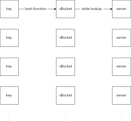
As shown in Figure 13-2, client requests for data identified with keys are mapped to vBuckets and not servers. The vBuckets in turn are mapped to servers. The hash function maps keys to vBuckets and allows for rebalancing as the number of vBuckets changes. At the same time, vBuckets themselves map to servers via a lookup table. Therefore, the vBuckets-to-server mapping is sort of stationary and the real physical storage of the data is not moved when vBuckets are reallocated.

Membase consists of the following components:

• ns_server — The core supervisor.
• Memcached and Membase engine — Membase builds on top of Memcached. The networking and protocol support layer is straight from Memcached and included in Membase. The Membase engine adds additional features like asynchronous persistence and support for the Telocator Alphanumeric Protocol (TAP).
• Vbucketmigrator — Based on how ns_server starts one or more vbucketmigrator processes, data is either replicated or transferred between nodes.
• Moxi — Memcached proxy with support for vBuckets hashing for client routing.

There is a lot more to Membase but hopefully you understand the very basics from this subsection so far. More of Membase architecture and performance is included in the following chapters.

In addition, bear in mind that Membase is now part of CouchBase, a merged entity created by the union of Membase and CouchDB. This union is likely to impact the Membase architecture in significant ways in the next few releases.

HYPERTABLE UNDER THE HOOD

Hypertable is a high-performance alternative to HBase. The essential characteristics of Hypertable are quite similar to HBase, which in turn is a clone of the Google Bigtable. Hypertable is actually not a new project. It started around the same time as HBase in 2007. Hypertable runs on top of a distributed filesystem like HDFS.

In HBase, column-family-centric data is stored in a row-key sorted and ordered manner. You also learned that each cell of data maintains multiple versions of data. Hypertable supports similar ideas. In Hypertable all version information is appended to the row-keys. The version information is identified via timestamps. All data for all versions for each row-key is stored in a sorted manner for each column-family.

Hypertable provides a column-family-centric data store but its physical storage characteristics are also affected by the notion of access groups. Access groups in Hypertable provide a way to physically store related column data together. In traditional RDBMS, data is sorted in rows and stored as such. That is, data for two contiguous rows is typically stored next to each other. In column-oriented stores, data for two columns is physically stored together. With Hypertable access groups you have the flexibility to put one or more columns in the same group. Keeping all columns in the same access group simulates a traditional RDBMS environment. Keeping each column separate from the other simulates a column-oriented database.

Regular Expression Support

Hypertable queries can filter cells based on regular expression matches on the row-key, column qualifier, and value. Hypertable leverages Google’s open-source regular expression engine, RE2, for implementing regular expression support. Details on RE2 can be accessed online at http://code.google.com/p/re2/. RE2 is fast, safe, and thread-friendly regular expression engine, which is written in C++. RE2 powers regular expression support in many well known Google products like Bigtable and Sawzall.

RE2 syntax supports a majority of the expressions supported by Perl Compatible Regular Expression (PCRE), PERL, and VIM. You can access the list of supported syntax at http://code.google.com/p/re2/wiki/Syntax.

Some tests (http://blog.hypertable.com/?p=103) conducted by the Hypertable developers reveal that RE2 was between three to fifty times faster than java.util.regex.Pattern. These tests were conducted on a 110 MB data set that had over 4.5 million unique IDs. The test results can vary depending on the data set and its size but the results are indicative of the fact that RE2 is fast and efficient.

Many concepts in Hypertable and HBase are the same and so repeating those same concepts here is not beneficial. However, a passing reference to an idea that is important in both places but not discussed yet is that of a Bloom Filter.

Bloom Filter

Bloom Filter is a probabilistic data structure used to test whether an element is a member of a set. Think of a Bloom Filter as an array of m number of bits. An empty Bloom Filter has a value of 0 in all its m positions. Now if elements a, b, and c are members of a set, then they are mapped via a set of k hash functions to the Bloom Filter. This means each of the members, that is a, b, and c are mapped via the k different hash functions to k positions on the Bloom Filter. Whenever a member is mapped via a hash function to a specific position in the m bit array the value in that particular position is set to 1. Different members, when passed through the hash functions, could map to the same position in the Bloom Filter.

Now to test if a given element, say w, is a member of a set, you need to pass it through the k hash functions and map the outcome on the Bloom Filter array. If the value at any of the mapped positions is 0, the element is not a member of the set. If the value at all the positions is 1, then either the element is a member of the set or the element maps to one or more position where the value was set to 1 by another element. Therefore, false positives are possible but false negatives are not.

Learn more about Bloom Filter, explained in the context of PERL, at www.perl.com/pub/2004/04/08/bloom_filters.html.

APACHE CASSANDRA

Apache Cassandra is simultaneously a very popular and infamous NoSQL database. A few examples that used Cassandra in the early part of the book introduced the core ideas of the store. In this section, I review Cassandra’s core architecture to understand how it works.

Peer-to-Peer Model

Most databases, including the most popular of NoSQL stores, follow a master-slave model for scaling out and replication. This means for each set, writes are committed to the master node and replicated down to the slaves. The slaves provide enhanced read scalability but not write scalability.

Cassandra moves away from the master-slave model and instead uses a peer-to-peer model. This means there is no single master but all the nodes are potentially masters. This makes the writes and reads extremely scalable and even allows nodes to function in cases of partition tolerance. However, extreme scalability comes at a cost, which in this case is a compromise in strong consistency. The peer-to-peer model follows a weak consistency model.

Based on Gossip and Anti-entropy

Cassandra’s peer-to-peer scalability and eventual consistency model makes it important to establish a protocol to communicate among the peers and detect node failure. Cassandra relies on a gossip-based protocol to communicate among the nodes. Gossip, as the name suggests, uses an idea similar to the concept of human gossip. In the case of gossip a peer arbitrarily chooses to send messages to other nodes. In Cassandra, gossip is more systematic and is triggered by a Gossiper class that runs on the basis of a timer. Nodes register themselves with the Gossiper class and receive updates as gossip propagates through the network. Gossip is meant for large distributed systems and is not particularly reliable. In Cassandra, the Gossiper class keeps track of nodes as gossip spreads through them.

In terms of the workflow, every timer-driven Gossiper action requires the Gossiper to choose a random node and send that node a message. This message is named GossipDigestSyncMessage. The receiving node, if active, sends an acknowledgment back to the Gossiper. To complete gossip, the Gossiper sends an acknowledgment in response to the acknowledgment it receives. If the communication completes all steps, gossip successfully shares the state information between the Gossiper and the node. If during gossip the communication fails, it indicates that possibly the node may be down.

To detect failure, Cassandra uses an algorithm called the Phi Accrual Failure Detection. This method of detection converts the binary spectrum of node alive or node dead to a level in the middle that indicates the suspicion level. The traditional idea of failure detection via periodic heartbeats is therefore replaced with a continuous assessment of suspicion levels.

Whereas gossip keeps the nodes in sync and repairs any temporary damages, more severe damages are identified and repaired via an anti-entropy mechanism. In this process, data in a column-family is converted to a hash using the Merkle tree. The Merkle tree representations compare data between neighboring nodes. If there is a discrepancy, the nodes are reconciled and repaired. The Merkle tree is created as a snapshot during a major compaction operation.

This reconfirms that the weak consistency in Cassandra may require reading from a Quorum to avoid inconsistencies.

Fast Writes

Writes in Cassandra are extremely fast because they are simply appended to commit logs on any available node and no locks are imposed in the critical path. A write operation involves a write into a commit log for durability and recoverability and an update into an in-memory data structure. The write into the in-memory data structure is performed only after a successful write into the commit log. Typically, there is a dedicated disk on each machine for the commit log because all writes into the commit log are sequential and so we can maximize disk throughput. When the in-memory data structure crosses a certain threshold, calculated based on data size and number of objects, it dumps itself to disk.

All writes are sequential to disk and also generate an index for efficient lookup based on a row-key. These indexes are also persisted along with the data. Over time, many such logs could exist on disk and a merge process could run in the background to collate the different logs into one log. This process of compaction merges data in SSTables, the underlying storage format. It also leads to rationalization of keys and combination of columns, deletions of data items marked for deletion, and creation of new indexes.

Hinted Handoff

During a write operation a request sent to a Cassandra node may fail if the node is unavailable. A write may not reconcile correctly if the node is partitioned from the network. To handle these cases, Cassandra involves the concept of hinted handoff. Hinted handoff can best be explained through a small illustration so let’s consider two nodes in a network, X and Y. A write is attempted on X but X is down so the write operation is sent to Y. Y stores the information with a little hint, which says that the write is for X and so please pass it on when X comes online.

Basho Riak (see www.basho.com/products_riak_overview.php) is another Amazon Dynamo inspired database that also leverages the concept of hinted handoff for write reconciliation.

Besides the interesting and often talked about Cassandra features and the underlying internals, I also need to mention that Cassandra is built on Staged Event-Driven Architecture (SEDA). Read more about SEDA at www.eecs.harvard.edu/~mdw/proj/seda/.

The next product I cover is a good old key/value store, Berkeley DB. Berkeley DB is the underlying storage for many NoSQL products and Berkeley DB itself can be used as a NoSQL product.

BERKELEY DB

Berkeley DB comes in three distinct flavors and supports multiple configurations:

• Berkeley DB — Key/value store programmed in C. This is the original flavor.
• Berkeley DB Java Edition (JE) — Key/value store rewritten in Java. Can easily be incorporated into a Java stack.
• Berkeley DB XML — Written in C++, this version wraps the key/value store to behave as an indexed and optimized XML storage system.

Berkeley DB, also referred to as BDB, is a key/value store deep in its guts. Simple as it may be at its core, a number of different configurations are possible with BDB. For example, BDB can be configured to provide concurrent non-blocking access or support transactions. It can be scaled out as a highly available cluster of master-slave replicas.

BDB is a key/value data store. It is a pure storage engine that makes no assumptions about an implied schema or structure to the key/value pairs. Therefore, BDB easily allows for higher-level API, query, and modeling abstractions on top of the underlying key/value store. This facilitates fast and efficient storage of application-specific data, without the overhead of translating it into an abstracted data format. The flexibility offered by this simple, yet elegant design, makes it possible to store structured and semi-structured data in BDB.

BDB can run as an in-memory store to hold small amounts of data or it can be configured as a large data store, with a fast in-memory cache. Multiple databases can be set up in a single physical install with the help of a higher-level abstraction, called an environment. One environment can have multiple databases. You need to open an environment and then a database to write data to it or read data from it. You should close a database and the environment when you have completed your interactions to make optimal use of resources. Each item in a database is a key/value pair. The key is typically unique but you could have duplicates. A value is accessed using a key. A retrieved value can be updated and saved back to the database. Multiple values are accessed and iterated over using a cursor. Cursors allow you to loop through the collection of values and manipulate them one at a time. Transactions and concurrent access are also supported.

The key of a key/value pair almost always serves as the primary key, which is indexed. Other properties within the value could serve as secondary indexes. Secondary indexes are maintained separately in a secondary database. The main database, which has the key/value pairs, is therefore also sometimes referred to as the primary database.

BDB runs as an in-process data store, so you statically or dynamically link to it when accessing it using the C, C++, C#, Java, or scripting language APIs from a corresponding program.

Storage Configuration

Key/value pairs can be stored in four types of data structures: B-tree, Hash, Queue, and Recno.

B-Tree Storage

A B-tree needs little introduction but if you do need to review its definition, read a freely available resource on B-tree online at www.bluerwhite.org/btree/. It’s a balanced tree data structure that keeps its elements sorted and allows for fast sequential access, insertions, and deletions. Keys and values can be arbitrary data types. In BDB the B-tree access method allows duplicates. This is a good choice if you need complex data types as keys. It’s also a great choice if data access patterns lead to access of contiguous or neighboring records. B-tree keeps a substantial amount of metadata to perform efficiently. Most BDB applications use the B-tree storage configuration.

Hash Storage

Like the B-tree, a hash also allows complex types to be keys. Hashes have a more linear structure as compared to a B-tree. BDB hash structures allow duplicates.

Whereas both a B-tree and a hash support complex keys, a hash database usually outperforms a B-tree when the data set far exceeds the amount of available memory because a B-tree keeps more metadata than a hash, and a larger data set implies that the B-tree metadata may not fit in the in-memory cache. In such an extreme situation the B-tree metadata as well as the actual data record itself must often be fetched from files, which can cause multiple I/Os per operation. The hash access method is designed to minimize the I/Os required to access the data record and therefore in these extreme cases, may perform better than a B-tree.

Queue Storage

A queue is a set of sequentially stored fixed-length records. Keys are restricted to logical record numbers, which are integer types. Records are appended sequentially allowing for extremely fast writes. If you are impressed by Apache Cassandra’s fast writes by appending to logs, give BDB with the queue access method a try and you won’t be disappointed. Methods also allow reading and updating effectively from the head of the queue. A queue has additional support for row-level locking. This allows effective transactional integrity even in cases of concurrent processing.

Recno Storage

Recno is similar to a queue but allows variable-length records. Like a queue, Recno keys are restricted to integers.

The different configurations allow you to store arbitrary types of data in a collection. There is no fixed schema other than those imposed by your model. In the extreme situation, you are welcome to store disparate value types for two keys in a collection. Value types can be complex classes, which could represent a JSON document, a complex data structure, or a structured data set. The only restriction really is that the value should be serializable to a byte array. A single key or a single value can be as large as 4 GB in size.

The possibility of secondary indexes allows filtering on the basis of value properties. The primary database does not store data in a tabular format and so non-existing properties are not stored for sparse data sets. A secondary index skips all key/value pairs that lack the property on which the index is created. In general, the storage is compact and efficient.

SUMMARY

Although only a few aspects of the internals of multiple databases were covered in this chapter, it’s not inaccurate to apply the same ideas to other stores. Architecture and under-the-hood exploration can be done at multiple levels of depth, starting from conceptual overview to in-depth code tours. I am mostly restricted to conceptual levels to make the chapter accessible to all. But this overview should give you the tools and knowledge to begin your own explorations.