11.4 Measurement System Analysis

In the preceding section we focused on identifying the sources of uncertainty. We also discussed the ways in which different types of uncertainties can be handled. The time has now come to quantify how great the uncertainty is. Before we have determined the accuracy and precision of our measurement system we do not know if it is sufficient for our purpose.

As the precision reflects a random variation between measurements, it is obtained by replicating the same measurement many times. These replicates should be taken at different times to include as many sources of noise as possible. External noises, especially, tend to vary over time. They arise through small variations in the environment, difficulties in repeating experimental settings and so on. This means that consecutive measurements tend to be more similar to each other than measurements made at different occasions, so they underestimate the effects of external noises. One of the better ways to assess the precision is to run regular stability checks during the measurements – a procedure that will be described further at the end of the next section.

Let us say that we are interested in the precision of the measurements with the bathroom scales above. This is obtained by weighing the same person at a number of different occasions. The person's weight will of course fluctuate from day to day depending on food intake and so on, so it may be tempting to use a constant weight instead of a person. By doing that we would exclude the natural variation in the person's weight from the measurement system. This may or may not be appropriate, depending on which part of the uncertainty we are interested in. We should be aware that excluding this variation leads to an underestimate of the total variation in the measurements.

Imagine that the purpose of our measurements is to test the weight-reducing effect of a diet. This effect is likely to manifest itself as a trend over several weeks. In that case the day-to-day fluctuations must be included when assessing the precision, because it tells us how large the effect must be to stand out from the noise. If the purpose is to measure the day-to-day fluctuations, on the other hand, this variation should of course not be included in the assessment. In the end, it is a matter of judgment which sources of variation to include.

One of the most common methods for improving the precision in a measured value is to average over several measurements. Although this does not decrease the variation in the data, it provides a more reliable estimate of the true value. The underlying reason is the central limit effect (Chapter 7). It is important to distinguish between the precision in the raw data and in the estimated value.

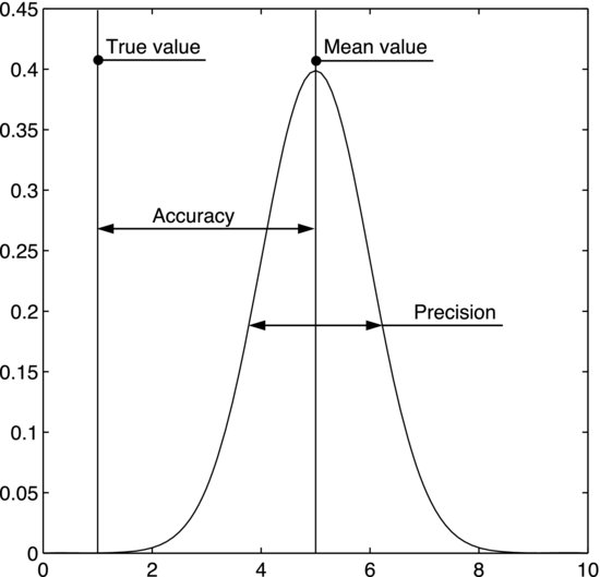
Determining the accuracy involves comparisons. For example, if you want to measure the concentration of a certain substance, the accuracy is obtained by measuring a sample of known concentration. The offset between the measured value and the true one is a measure of the accuracy. This procedure is used when calibrating a measurement system, where the accuracy is improved by adding a calibration constant to the measured value to eliminate the offset. Note that, whereas increasing the sample size may increase the precision in the measured value, it has no effect on the accuracy. The difference between precision and accuracy is illustrated in Figure 11.6.

Figure 11.6 The normal distribution represents the measurements. The accuracy is given by the distance between the distribution mean and the true value. The precision is given by the variation in the measurements.

It is not always possible to produce a well-defined standard for calibration in the laboratory. If you are interested in measuring the concentration of a short-lived radical in a flame, for example, you are facing the practical problem that flame radicals may cease to exist only nanoseconds after being formed. This makes it difficult to produce a sample of known concentration. In such cases it is strictly impossible to establish the accuracy in absolute units, but corrections may still be necessary to remove bias and to improve the relative accuracy. This can be illustrated by the beetle experiment, which is an example of a study based on relative comparisons. Only relative numbers are needed to differ between situations where the beetle can and cannot orient itself. The rolling time is merely an indirect measure of how straight the rolling path is. As long as the rolling times for straight and convoluted paths are substantially different, this indirect measure is fully sufficient to make an unambiguous distinction between the two situations. As a matter of fact, absolute units are not at all interesting in this context. We could make the distinction equally well using a clock going at the wrong rate. But even though the experiment was based on relative data, Example 11.3 showed that the rolling times needed a temperature correction to remove a bias that could otherwise have made the relative comparison less accurate. Even in cases where measurements cannot be calibrated in absolute units it is important to consider the relative accuracy.

When we have established the precision, our next question is if it is sufficient for the purpose of the experiment. The precision determines how small a difference you can detect between two sets of data. As previously stated, the precision in an averaged value is improved by increasing the sample size. We can determine the sample size required for detecting a certain difference using a technique called power analysis. It was discussed in a separate section of Chapter 8.

Sometimes we find that the precision of our measurement system must be improved. In such cases, the techniques presented in the last section become helpful. They helped us identify the components most likely to affect the uncertainty. These will now be the subject of more focused investigation. Let us say that we suspect the operator has an influence that decreases the precision. This may be investigated by letting different operators run several replicates of the same tests in random order. If there are differences between them this should now be seen in a t-test or, if there are more than two operators, a one-way ANOVA. If we suspect several sources of error we could use the type of analysis described in the measurement system analysis section of Chapter 8. In that example, an engine laboratory investigated if the control unit or the operator affected the measurements. A two-way ANOVA revealed whether or not there was a statistically significant effect of either of the variables. The error standard deviation gave us the measurement precision within the groups, whereas the operator effect was given by the difference between the two blocks. These types of analyses can point to potential improvements of the measurement system.

If our aim is to improve the precision, we need to quantify individual components of the uncertainty. This will involve isolated assessments of certain parts in the measurement chain. We could, for instance, suspect that the rack and pinion mechanism of the bathroom scales makes a substantial contribution to the overall error. To find out, we must find a way to investigate this part separately from the rest of the scales. By taking repeated measurements when exposing it to one and the same treatment we will get a measure of how much uncertainty it feeds into the measurement process. When we find components that are responsible for a large portion of the overall variation we know where to focus our improvement efforts.

There are different ways to express measurement precision. As explained in Chapter 7, the standard deviation is one of the more convenient measures of the amount of variability in a data set. Firstly, if the error is normally distributed the standard deviation can be used to identify outliers. This is because it is very unlikely to find values more than three standard deviations from the mean of a normally distributed sample. It is also convenient that the standard deviation has the same unit as the measured value. If we instead want to express the uncertainty of values that are averaged over a sample, the standard error of the mean is a better measure than the standard deviation. You may, for example, average your weight readings over a whole week to obtain a more reliable value. It is not the variation in the data set that is important in this case but how well the population mean is estimated. We obtain the standard error of the sample mean, , by dividing the sample standard deviation, s, by the square root of the sample size, n:

(11.2)

Here, s is an estimate of the population standard deviation, σ, and the reason that this formula estimates the error in the sample mean is given by the central limit theorem (Chapter 7). Yet another way to express the uncertainty is to use a confidence interval. Remember that these rules are not strict, so it is advisable to always state which error estimate you are using.

If the output value from an experiment is calculated from several measured values, evaluating the uncertainty can be considerably more complex. The total variation can then be calculated from the measurement variation using what is called error propagation analysis. Say that the value of interest, f, is a function of the two independent, measured variables, x1 and x2. If the error variances of these variables are σ12 and σ22, respectively, the error variance of f(x1, x2) is approximately given by:

(11.3)

The terms in the brackets are partial derivatives, meaning derivatives of f with respect to one of the variables when the other is held constant. This formula can be extended to any number of independent variables. To make the calculation more concrete, consider a situation where we are interested in determining the volume, V, of a cylinder from its measured diameter, d, and height, h. Call the error variances of these measures σd2 and σh2, respectively. The volume is given by:

(11.4)

The partial derivative of V with respect to d is:

(11.5)

Similarly, the partial derivative with respect to h is:

(11.6)

This means that the error variance in V is approximately given by:

(11.7)

Which of the two error variances on the right contributes most to the overall uncertainty clearly depends on the values of d and h.