8.4 The t-Test for One Sample
Let us revisit Exercise 6.5, where Sven claimed that the fuel consumption of his diesel car was less than 6.0 liters per 100 km. In the summer, he measured the following fuel consumptions in liters per 100 km:
![]()
In the exercise we were asked to determine if his claim was right. When I give this exercise to students after a lecture covering descriptive statistics, similar to how it was presented in Chapter 7, most course participants approach the exercise using descriptive statistics. They try to use the mean and standard deviation of the sample to answer the question. Typically, one half of a class concludes that Sven is right since the mean fuel consumption is below 6.0. The other half argues that, since some values are above 6.0, his claim must be incorrect. Although many students are hesitant to draw a definite conclusion, most are leaning towards one of these alternatives. They seldom claim that the question is wrongly posed.
Is it reasonable that researchers who are faced with the same problem and the same data arrive at completely different conclusions? Of course not, since the differences result from arbitrary and subjective considerations. After discussing this situation, some students revise their opinion and say that these data are insufficient to draw a conclusion.
Firstly, we might ask ourselves which number of measurements would be sufficient to draw a conclusion. A hundred? Once again, if we only know about descriptive statistics this is just a matter of taste. Secondly, has anyone considered how a hundred measurements would affect Sven's marriage? This may sound like a humorous remark but the fact is that it costs both time and money to collect data. It is necessary at some point to decide how much effort it is reasonable to invest in our measurements.
The aim of these anecdotes is not to amuse ourselves at the expense of other people but to point out how difficult it can be to draw conclusions using descriptive statistics. We are now starting to realize that we need a different approach to solve this problem.
Just as in the tea experiment at the beginning of this chapter, we will start by considering what we can say about the distribution from which Sven's measurements were sampled. Firstly, we need to decide what we mean by the “real” fuel consumption of the car. This number is affected by a wealth of factors, including Sven's driving style and his typical drive cycle. The sample can tell us something about what the typical fuel consumption is when he is driving the car, where he is driving it. It will not tell us much about the fuel consumption when others are driving it elsewhere. The car itself does not have a “true” fuel consumption, since the driver is such an important part of the equation. Let's rephrase our question as follows: is the mean of the population from which Sven's fuel consumptions are sampled less than 6.0 liters per 100 kilometers? Since the variation in the fuel consumption is affected by many factors we will resort to the central limit effect and assume that it is normally distributed. Since our sample is small we may use the t-distribution. The mean ![]() and standard deviation s of our sample then represent an observed t-value:
and standard deviation s of our sample then represent an observed t-value:
Putting our s = 0.1643, ![]() = 5.98, and n = 5 into Equation 8.1 and letting the hypothetical mean μ be equal to 6.0, we obtain tobs = −0.27.
= 5.98, and n = 5 into Equation 8.1 and letting the hypothetical mean μ be equal to 6.0, we obtain tobs = −0.27.
The logic behind using the t-distribution is that the sample mean is expected to display some amount of random variation about the distribution mean, determined by the number of degrees of freedom. We use 6.0 liters per 100 km as a hypothetical distribution mean, since the claim is that the sample is drawn from a distribution with a mean different from this. The null hypothesis assumes that any deviation from the mean is due to random variation about the hypothetical mean. The significance test will determine whether this assumption may be rejected or not.
By rephrasing our question we have almost formulated our null hypothesis. Remember that we cannot prove that the fuel consumption is less than 6.0 liters per 100 km, but we may reject the statement that it is not based on a significance test. We will set up the following two hypotheses:
(8.2) ![]()
H0 is the null hypothesis and assumes that the claim is incorrect – that the distribution mean is equal to 6.0, or even higher. (As we are making a one-sided test, variation about a value higher than 6.0 will support the null hypothesis also). Ha is called the alternative hypothesis and it represents the effect that we want to demonstrate by giving the data a chance to reject the null hypothesis.
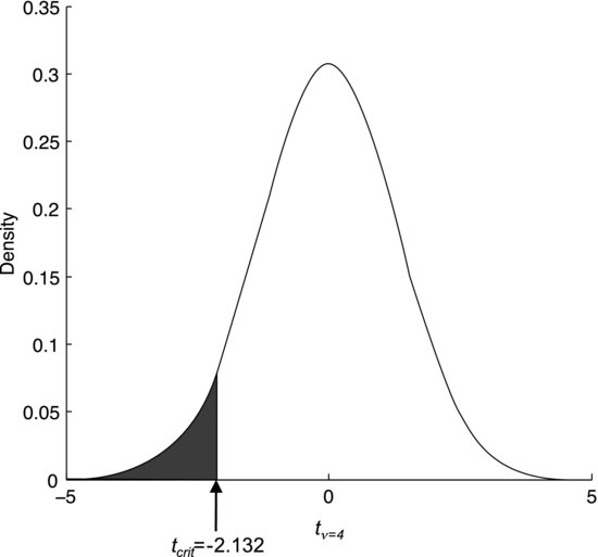
To make a significance test we need a critical t-value. If we want to test the null hypothesis at the 95% confidence level the probability of observing a t-value more extreme than the critical value should be α = 0.05. Looking in the table of probability points for the t-distribution in the Appendix, we find that tcrit = 2.132 for α = 0.05 and four degrees of freedom.
Two things should be noted. Firstly, since the consumption is claimed to be below a certain value we are assessing a one-sided interval. As there is only one way of being outside a one-sided interval, we are not using α/2 as we did for the two-sided confidence interval for blood pressures at the end of Chapter 7. Secondly, the table only provides positive t-values and we are testing for negative values. This is because we would reject the null hypothesis if our data were to yield a tobs at the far left of the distribution in Figure 8.2. However, since the t-distribution is symmetric about the mean we may simply mirror it through the origin to obtain the relevant tcrit of −2.132, which is marked in Figure 8.2.
Figure 8.2 The t-distribution connected with Sven's fuel consumption measurements in the summer.
We note that our tobs of −0.27 is less extreme than our tcrit of −2.132. This means that the data support the null hypothesis: the mean fuel consumption of Sven's car cannot be claimed to be less than 6.0 liters per 100 kilometers. This should come as no surprise, as you calculated a confidence interval for the mean fuel consumption in Exercise 6.9 that extended from 5.8 to 6.2 liters per 100 kilometers.
The analysis that we just went through is called a one-sample t-test. It is used when we want to compare a sample to a fixed standard, such as a target fuel consumption. Let us review how we did it. Firstly, we stated our problem as a practical question. Is the mean fuel consumption really less than 6.0 liters per 100 kilometers? Secondly, we formulated a null hypothesis based on our question. It assumed that the claim was incorrect and that any deviation from the hypothetical mean was due to random variation. A general rule to keep in mind when formulating the null hypothesis is that it always includes an equals sign. This is because it assumes that the true mean is equal to the hypothetical mean. In this case we made a one-sided test, meaning that the null hypothesis is rejected only if the data deviate significantly in a given direction from the hypothetical mean. Our null hypothesis was, therefore, that the mean of the distribution from which the data were drawn is equal to or greater than 6.0 liters per 100 kilometers.
Thirdly, we formulated an alternative hypothesis, representing the claim that we want to demonstrate. It is simply the opposite of the null hypothesis. Finally, we determined the observed and critical t-values. The observed t-value represents the data and the critical value represents the limit that it must exceed to be judged statistically significant. If tobs lies between the critical value and the hypothetical distribution mean, there is more than 95% probability that the data were drawn from that distribution. Such a result would support the null hypothesis.
Reading the critical t-value from a table is relatively easy but, as we have seen, it can be difficult to understand when tcrit should be negative. Unfortunately, we have to figure out if we are testing for positive or negative values ourselves. The easiest way to do it is to draw a bell-shaped curve to represent our reference distribution and visualize the sort of observations that would discredit the null hypothesis. For a two-sided test it is easy: the farther out in either tail the observed t-value lies, the less likely the null hypothesis is to be true. In one-sided tests it is necessary to understand if observations to the right or to the left of the mean are less likely under the null hypothesis. tcrit is positive if observations to the right would discredit the null hypothesis, otherwise it is negative. These scenarios are summarized in Table 8.2.
Table 8.2 When to reject the null hypothesis.
| Null hypothesis | Type of test | Reject H0 if: |
| μ ≤ μ0 | One-sided | tobs > tcrit |
| μ ≥ μ0 | One-sided | tobs < -tcrit |
| μ = μ0 | Two-sided | tobs < - tcrit or tobs > tcril |
When hypothesis tests are performed using statistical software the result is often presented as a so-called p-value. This value is just the probability that the sample in question was drawn from the distribution associated with the null hypothesis. The lower this probability is, the less credible the null hypothesis becomes. The p-value of tcrit is, by definition, our α-value (usually 0.05). If tobs is more extreme than tcrit, p will be lower than α. This outcome supports the alternative hypothesis and the result is said to be statistically significant. Interpreting the p-value is often confusing to beginners, as it may seem counter-intuitive that a low probability represents a statistically significant result. As researchers we are generally more interested in the alternative hypothesis. It is important to remember that the p-value is the probability of obtaining data that are at least as extreme as the ones in the sample, assuming that the null hypothesis is correct. If you are in doubt you may find the following mnemonic helpful:
![]()
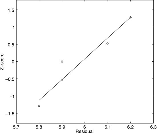
Before leaving the one-sample t-test it is appropriate to mention that our use of the t-distribution relies on the assumption that the data are reasonably normally distributed. This is often a fair assumption but it is best to convince oneself before continuing the test. The easiest way to do it is to make a normal plot of the data since it may be difficult to judge the normality from a histogram when the sample is small. It is a general recommendation to always plot your data before analyzing them, as a graphical representation provides a better overview over the distribution and relationships in the data than the numbers themselves.
You should not expect all the points to adhere closely to a straight line in the normal plot but you should look out for obvious signs that there is skewing. Even severely skewed samples may be useful, as skewing often can be remedied by a data transformation, such as taking the logarithm of the data or something similar. It is also good to know that moderate violations of normality are not a concern. All hypothesis tests presented in this chapter are robust to non-normality, especially when the sample size increases. Figure 8.3 shows a normal plot of the fuel consumption data. This sample is too small to allow an accurate assessment of the normality but at least there are no apparent signs of skewing.
Figure 8.3 Normal plot for the fuel consumption data.