8.5 The Power of a Test

As we have seen, it is possible that extreme values occur purely by chance. This means that there is a small probability that our significance test rejects the null hypothesis even when it is true. This is called a Type I error and the probability of making one is, of course, equal to our significance level, α. This may be illustrated using Figure 7.15, which represents the reference distribution connected with a null hypothesis. It is perfectly possible to obtain values in the shaded tails of this distribution also when the null hypothesis is true, but our significance test will reject the null hypothesis when values that occur with a probability of less than α = 0.05 are drawn.

When designing an experiment it is also important to be aware of a different risk: that of accepting the null hypothesis when it is, in fact, false. This is called a Type II error and the probability of making one is represented by the symbol β. Figure 8.4 illustrates how this risk occurs. The solid curve on the right is the reference distribution associated with the null hypothesis. It could, for example, be the t-distribution connected with Sven's fuel consumptions if the true mean were 6.0 liters per 100 km. Let us say that the null hypothesis is false. This means that we are sampling from another population, which is represented by the left, dashed curve. In actual situations we never know exactly which distribution we are sampling from, so it is only drawn here for illustration. The significance test tells us nothing of the real distribution – it only tells us whether it is probable that we are sampling from the reference distribution or not.

Figure 8.4 Illustration of how the β-risk occurs. When sampling from the left distribution, some tail values appear to support the null hypothesis although it is false. The null hypothesis is connected with the right distribution.

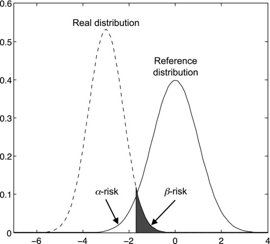
What complicates the situation in Figure 8.4 is that the tails of the two distributions overlap. We may therefore obtain a value from the real distribution that could have been drawn from the reference distribution with a probability greater than α. The null hypothesis would then appear to be supported by the data although it is false. A shaded area in the tail of the left distribution in Figure 8.4 represents the probability β of obtaining such a value from the left distribution. This probability is also known as the β-risk. The white area under the tail of the reference distribution represents α.

In practical terms, this means that there is always a certain probability that a real effect remains undetected in your experiment. When you design your experiment you must decide how large a β you are willing to accept. What should the probability be of letting the effect go undetected? Zero is not an option.

Figure 8.4 shows us that the β-risk depends on the overlap between the two distributions. This, in turn, depends on the significance level α, the difference δ between the distribution means, and their respective widths. According to the central limit theorem the width decreases with increasing sample size. This means that the smaller δ is, the larger a sample you will need to detect it.

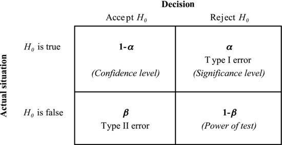
Figure 8.5 summarizes the four categories of possible outcomes of an experiment. On the left we have the two possibilities for the null hypothesis: it is either true or false. The two decisions that are possible to make based on the data are given at the top: the null hypothesis is either accepted or rejected. As we have mentioned, two of the outcomes are incorrect. A Type I error, rejecting the null hypothesis when it is true, occurs with probability α. A Type II error, accepting the null hypothesis when it is false, occurs with probability β. This leaves two categories of correct outcomes. Accepting the null hypothesis when it is true occurs with probability 1 – α, which we refer to as the confidence level of our test. The last category, rejecting the null hypothesis when it is false, occurs with probability 1 – β. This number is called the power of the test. Just as 95% is a conventional confidence level in many experiments, 80% is a typical power, but both these numbers may vary according to the situation. In applications like medicine and aerospace engineering, where it is highly important to avoid errors, higher confidence levels and powers are often used.

Figure 8.5 α is the probability of a Type I error, β the probability of a Type II error. These probabilities define the power, significance level and confidence level of the test.

If you find it difficult to remember these categories of error, it might be useful to compare an experiment to a court of law. For the prosecutor, the purpose of a trial is to give the evidence a chance to reject the “null hypothesis” that the suspect is innocent. A Type I error then corresponds to convicting a suspect that is, in fact, innocent. Freeing a guilty person would be a Type II error. Just as in experiments, one way for the prosecutor to minimize this risk is to gather more evidence against the suspect.

The problem that remains is to determine how large a sample we need to detect a certain difference, δ, between two population means at a certain level of power. Most statistical software contains a function that does this, which is often called “power and sample size” or something similar. It typically requires that we specify four of the five parameters α, 1 − β, δ, the standard deviation, and the sample size. Based on these it calculates the fifth for us.

The standard deviation describes how far the estimated mean deviates from the true mean. This is not known in practice, so the power analysis can be seen as a play with probabilities. It shows what would happen if the true standard deviation were the one that we specify. Let's use Sven's fuel consumptions as an example. The sample size is five. The standard deviation of the mean is estimated by the sample standard deviation divided by the square root of five. Say that we are interested in using a significance level, α, of 0.05 and a power, 1-β, of 0.8. Plugging these values into the power analysis of a statistical software package returns the fifth parameter, δ = 0.12. This means that, with the specified standard deviation and sample size, the true mean has to deviate by more than 0.12 from the hypothetical mean (6.0 liters per 100 km) to be considered different from it. In Sven's data the difference, δ, between the sample mean and the hypothetical mean is only 0.02 liters per 100 km. How large a sample would be needed to detect this difference? Using the same standard deviation, α, and β as before, the software returns a sample size of 108. Sven's data set is indeed insufficient to reveal a difference this small.