
9.5 Factor Screening: Fractional Factorial Designs
At the beginning of a study it is often possible to think of a large number of factors that could be important for the response. Initially, we may only be interested in finding out which of these candidates – if any – have a substantial effect. This process of separating the vital few factors from the trivial many is called screening. The purpose is to find out which factors to keep for the real experiment, which is to be conducted later.
Equation 9.2 shows that the number of runs in a full factorial experiment increases exponentially with the number of factors. This is why it is convenient to use special screening designs to reduce the number of runs. We will soon see that this is done by “mixing effects together” and focusing on main effects and low order interactions. These designs typically fall into two categories: fractional factorial designs and Plackett–Burman designs. We will concentrate on the first category and only briefly mention some characteristics of the latter.
The 23 design in Table 9.3 tests three factors in eight runs (replicates have been left out for simplicity). Imagine that you are interested in four factors but are only allowed eight runs. What would you do? The whole matrix corresponds to the complete information set for a 23 design, so the fourth factor must come from one of these columns. Our rule of thumb tells us that the highest order interactions are probably not carrying any information when n increases beyond three. This means that the three-way interaction ABC is least likely to carry any information. We could “cheat” and simply call the ABC column D, and vary our fourth factor according to it. We obtain a design that tests the influence of four factors in only eight runs – half of what would be needed in a true full factorial design. It was obtained by confounding or aliasing the factor D with ABC. We will now briefly discuss some implications of this.
First of all we should note that the interaction ABC could have an effect on the response, even though it is not very likely. If so, we cannot separate this effect from the effect of D since they are completely mixed up with each other. In mathematical terms, ABC and D are perfectly correlated. But this is only the beginning. Table 9.5 shows the set of interactions for the new design, rearranged to highlight additional confounding. We see that not only is D confounded with ABC but that each main effect is confounded with a three-way interaction. We also see that the AB column is identical to the CD column. The same is true of AC and BD, and of BC and AD. When confounding D with ABC we have introduced confounding in all other terms as well. This means that the design is not orthogonal anymore – all effects are blended with other effects.
Table 9.5 Two-level half factorial design with four factors. The columns have been rearranged to highlight the confounding.
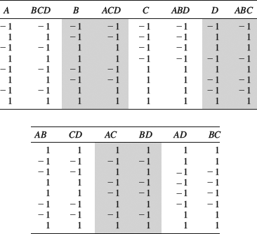
By confounding D with ABC we have generated a design that allows us to test the influence of four factors with half the number of runs that would be required for a full factorial design. The design is therefore called a half factorial design. It is also referred to as a 24–1 design, since it is a two-level design testing four factors in 24–1 = 8 runs. Reducing the number of runs even more we would get a quarter factorial design (24–2). These types of reduced designs are generally referred to as fractional factorial designs. The test matrix in Table 9.5 is analyzed in exactly the same way as the full factorial design, obtaining effects by taking the inner products of the columns and the response. The big difference is that the interactions are mixed up with each other. If AB seems to be significant, we do not know if AB or CD is responsible for the effect. We simply pay for reducing the number of runs by obtaining less detailed information.
In addition to reducing the size of an experiment, confounding is a suitable method for introducing a block variable. This is because the confounding disappears if the block variable turns out to be unimportant. The experiment then provides more detailed information about the remaining factors.