Chapter 5

Continuous-Time LTI Systems and the Convolution Integral

In This Chapter

Understanding the general input/output relationship

Digging into the convolution integral and its properties

Working with the step response, impulse response, and stability implications

Ready to get pumped up on what you can do in the time domain with linear time-invariant (LTI) systems?

The starting point is the convolution integral, the main time-domain tool for relating the output of a system to its input in combination with the impulse response (IR). In other words, the IR enables you to calculate a system’s output in terms of the input. You can use the IR in different ways; one way is convolution.

In this chapter, I describe the relationship between the impulse response and convolution integral and introduce properties related to these concepts. I also provide tips on how to manage the nitty-gritty details of convolution.

The mechanics of the convolution integral are tedious, no doubt, so I provide several worked-through examples and include information about computer tools that can help you evaluate the convolution integral and self-check your plotting work. I also scratch the surface of a powerful stability theorem for LTI systems that relies almost solely on the IR. This theorem grows even more powerful in Chapter 13 when it’s combined with the Laplace transform.

Establishing a General Input/Output Relationship

A general continuous-time system input/output relationship is described mathematically as where represents the system or operator of interest. Figure 5-1 depicts this relationship in block diagram form. The operator describes a mapping of the input sequence, x(t), to the output sequence, y(t).

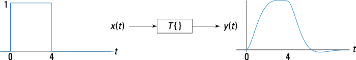
Figure 5-1: Block diagram depicting a general input/output relationship.

In Chapter 3, I define what it means for a system to be both linear and time-invariant (LTI). For LTI systems, the in Figure 5-1 is replaced by to signify that the systems of focus in this chapter are LTI.

The business of developing a general input/output relationship in this section begins with the definition of impulse response because, with the impulse response in hand, you can develop the convolution integral as a means to calculate the system output for any input and the impulse response.

Developing the convolution integral requires both the linearity and time invariance assumptions. I show you the steps in this important development. I also touch on useful properties of the convolution integral.

LTI systems and the impulse response

The impulse response is the beating heart of signals and systems work for LTI systems. Here’s why: If you know the impulse response for any LTI system, you can use that information to figure out the system’s response to any input. This is a really big super enormous deal.

The impulse response of a continuous-time LTI system, h(t), for example, is defined as the output produced by an at-rest system, when given input . The signal is the unit impulse (see Chapter 3). The at-rest condition ensures that the resulting h(t) is due solely to the input signal. Figure 5-2 shows how to find the impulse response.

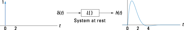
Figure 5-2: Finding the impulse response.

Mathematically, Figure 5-2 tells you that . This information along with any input x(t) allows you to calculate the system output y(t).

Developing the convolution integral

To get y(t) from x(t) and h(t), start with the sifting property (see Chapter 3) representation of x(t) and then form a numerical approximation to the integral:

Figure 5-3 shows a rectangular partition approximation to the sifting property integral representation of x(t), with replaced by and replaced by .

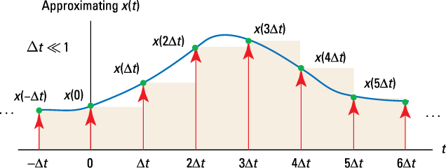
Figure 5-3: Time-shifted impulse approximation to the sifting integral for .

Now you can operate on both sides of the x(t) integral approximation with the LTI system, , and in three steps establish the convolution integral:

1. On the left side, ; on the right side, take advantage of the linearity property:

When moves inside the sum, it finds as the only function of time t to operate on.

2. Take advantage of time invariance to write .

Time-invariant systems always give the same response, to within a time offset, that’s independent of time axis shifts.

3. Notice that the rectangular partition approximation to the input is now a linear combination of time-shifted impulse responses, , weighted by the sample values of the input.

Figure 5-4 shows the individual terms in the approximation, assuming h(t) is an exponential pulse, , decaying to zero for a > 0.

To formally get to the convolution integral, you let and let such that . The sum becomes the convolution integral with the limits running from to .

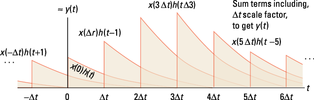
Figure 5-4: Approximat-ing y(t) as a sum of weighted and time-shifted impulse responses.

By letting as , you can replace the sum with an integral, and the approximation is exact:

The customary notation to indicate a convolution is :

By the change of variables, , you can also write the convolution integral as

Looking at useful convolution integral properties

The convolution integral obeys the standard commutative, associative, and distributive algebraic properties, as Table 5-1 shows:

Table 5-1 Convolution Integral Properties

Property	Algebraic Representation
Commutative
Associative
Distributive

You can find information on these properties in Chapter 6 in context of discrete-time systems and the convolution sum.

The commutative and associative properties also lead to the series/cascade and parallel connection block diagrams that are shown in Figure 5-5. The series/cascade connection result states that

The parallel connection results says

Additionally, linearity allows you to swap the order of the subsystems in the series connection.

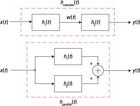
Figure 5-5: Block diagrams of series/cascade (a) and parallel (b) connections of LTI systems.

Convolution involving the unit impulse has some memorable outcomes, meaning you need to remember to take advantage of the simplicity of these convolution forms; you won’t regret it. The following identities hold:

---

---

Working with the Convolution Integral

Ready to jump in? In this section, I show you how to work through the details of convolution integral examples. And details, by the way, are especially important in convolution integrals, so be sure to follow each step. These examples rely heavily on signal flipping and shifting transformations. If you need a refresher on signal flipping and shifting, take a peek at Chapter 3.

Seeing the general solution first

To solve a convolution problem, you need to know one of the two forms of the integrand: . It all comes down to integrating the product of the two functions that form the integrand. As t increases from to , slides from left to right along the -axis. For each value of t, consider the product and integrate the nonzero or overlap intervals along the -axis.

For each t phrase sounds daunting at first, but contiguous intervals of t values occur where the integration on the -axis uses the same integration setup.

For the alternative integrand form, , do the same thing, except slides as t changes.

The solution is piecewise continuous, meaning expressions for are valid for some , which corresponds to case i, i = 1, . . . , N. When you put all the pieces together, you have a solution that’s valid for .

The four steps in Figure 5-6 outline the general solution procedure.

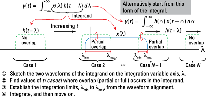
Figure 5-6: Solving a convolution integral problem in four steps with cases as slides from left to right.

You don’t want to mess up the sketching step because it provides a road map for all the analysis/calculations that follow. A bad sketch leads you along the wrong roads.

Example 5-1: To see the patterns of convolution problems for finite-duration signals, solve for the general support interval — the t-axis interval where . Here are some things to notice in Figure 5-7:

Figure 5-7a shows the signal and impulse response to be convolved.

Figure 5-7b shows both signals on the with t as a free variable.

Also in Figure 5-7b, the flipped and shifted waveform is positioned by selection of t (dashed line) at the start of overlap () and at the end of overlap ().

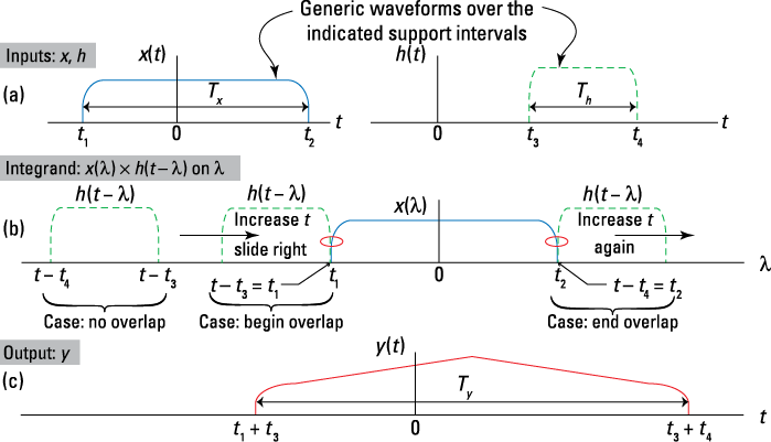
Figure 5-7: Convolving two generic finite length waveforms: the convolution inputs (a), the integrand waveforms along the -axis (b), and the output y(t) (c).

To calculate the convolution integral, using the form ,

follow the steps from Figure 5-6 but only in a general way because the exact waveform details aren’t available for this example.

1. Sketch the two waveforms of the integrand on the integration variable axis.

The example in Figure 5-7b sketches the two waveforms on the .

2. Find values of t (cases) where overlap (partial or full) occurs in the integrand.

Refer to the example in Figure 5-7: As t increases, the point of first overlap occurs when the leading edge of located at .

For , no overlap occurs, and the integrand is 0, meaning as well. As t continues to increase, eventually the trailing edge of is located at .

For , no overlap exists, and the integrand is again 0, so .

For , you’ll likely have more than one overlap case to consider, depending on the waveform shapes.

3. Establish the integration limits from the waveform alignment.

Integration limits are set by the specific cases, so they don’t apply in this example. In a gross sense, all you can say is that the fixed signal constrains the limits on to be .

4. Integrate, and then move on.

You don’t carry out the integration in this example.

A few things to note about the convolution result: The support interval for the output is at most . But you have no guarantee that for at least some values of t on this interval. The output starts at and ends at . The duration or length of the support interval is , which is the sum of the input signal durations.

Using the definitions established in Example 5-1, .

Solving problems with finite extent signals

This section contains examples for working convolution problems with real numbers, where both the signal and the impulse response are of finite duration.

Example 5-2: Convolve the rectangular pulse signals and (these are real signals), using the same form of the

convolution integral as Example 5-1: .

1. Sketch the two waveforms of the integrand on the integration variable axis.

Check out the waveforms sketched in Figure 5-8a and the signal product cases sketched in Figures 5-8b through 5-8f.

2. Find values of t (cases) where overlap (partial or full) occurs in the integrand.

Figure 5-8: The convolution of : the convolution inputs (a), and the integrand waveforms (b–f) under Cases 1–5, respectively.

For Example 5-2, you have five cases to consider:

• Case 1 and Case 5 occur when and , respectively. For Case 1, for , and for Case 5, for . As a check from the results of Example 5-1, the output starts at .

• Case 2 is what I call partial overlap leading edge. You need or for the active interval.

• Case 3 is full overlap or a straddle that occurs when . The active interval is .

• Case 4 is partial overlap trailing edge. This condition requires , so the active interval is .

3. Establish the integration limits from the waveform alignment.

With the help of Figure 5-6, the integration limits for each case fall into place quite easily.

• Under Case 2, the limits on are .

• Under Case 3, the limits on are set by , so just 3 to 4.

• Under Case 4, the limits on are .

4. Integrate, and then move on.

• The Case 2 integration is .

• The Case 3 integration is .

• The Case 4 integration is .

Pulling all the pieces together in one big case expression yields the following:

To plot , write a piecewise function in Python, using the IPython environment. First, create time axis vector, t, and pass it to the function example_5_2(t). You can see the results in Figure 5-9. The basic coding approach I use here is useful whenever you need to plot a piecewise function.

When faced with an unfamiliar waveform scenario, try visualizing your results as a troubleshooting aid. Assuming and are free of impulse functions, the plot of should be piecewise continuous, meaning no jumps between the waveform pieces.

In [187]: t = arange(0,8,0.05) # t from 0 to 8s

In [188]: def example_5_2(t): # embedded IPython function

     ...: y = zeros(len(t))

     ...: for k, tt in enumerate(t):

     ...: if tt >= 3 and tt < 4:

     ...: y[k] = 2*(tt - 3)

     ...: elif tt >= 4 and tt < 5:

     ...: y[k] = 2

     ...: elif tt >= 5 and tt < 6:

     ...: y[k] = 2*(6 - tt)

     ...: return y

In [189]: y = example_5_2(t) #call the function with t

In [190]: plot(t,y) # plot the results (you add labels)

When you first see the piecewise expression for , it may not be obvious that it describes a trapezoid-shaped waveform. The trapezoid height corresponds to the overlap area, . For identical rectangle pulse widths, such as , the convolution is a triangle. In particular, you

can show that , which is the triangle pulse that’s

defined in Chapter 3, scaled by T and of full base width of 2T.

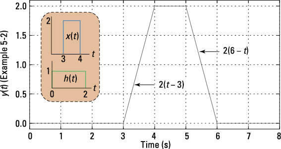
Figure 5-9: Piecewise plot of for Example 5-2 showing the trapezoid that results when rectangles are convolved.

As a modification to the rectangle input, let , which is a right triangle pulse shape. Because has support over the interval [0, 2], all work is reusable for Steps 1 through 3, so the five cases remain the same as well as the integration limits established for Cases 2 through 4. The changes come under Step 4 when you have to integrate. The integrand is now . With the integrand change, you get the following:

The waveform peak, which is the maximum overlap area of , is now the area of the triangle formed by , which is . Figure 5-10 shows that making triangular, smoother than the original rectangular pulse, results in a smoother .

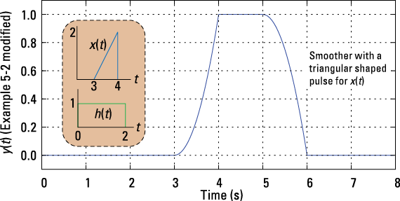
Figure 5-10: Piecewise plot of with now a right triangle shape.

To check your analysis, use the Python function conv_integral(x1,t1,x2,t2) in the module ssd.py at www.dummies.com/extras/signalsandsystems. With this function, you can numerically calculate the convolution integral by using simple rectangular integration. The time step when creating the t array needs to be small to achieve good numerical accuracy, as I did in Figure 5-10. Check out the code summary:

In [325]: t = arange(0,8,0.01) # create t axis, dt=0.01

In [326]: x = 2*(t - 3)*ssd.rect(t-3.5,1) # create x(t)

In [327]: h = ssd.rect(t-1,2) # create h(t)

In [328]: y,ty = ssd.conv_integral(x,t,h,t) # convolve

In [329]: plot(ty,y) # plot results

Dealing with semi-infinite limits

Distortion sometimes enters the picture when a simple system/filter has an exponential impulse response. The system time constant — the time it takes to decay from 1 to , 1/a (1 s in Example 5-12) — slows down the edges of the input pulse. For a fixed time constant, the pulse duration needs to be on the order of 10 times the time constant for the output pulse to resemble the input.

In the real world, a wired network (Ethernet) connection relies on a twisted-pair cable to transfer digital pulses from one end to the other. The cable acts as a filter similar to the exponential impulse response of this example. Trying to send pulses (symbols) at too high a rate, , results in pulse distortion. Too much pulse distortion increases the chance of symbols being received in error.

Example 5-3: Consider and . The convolution integral form is .

I’d rather flip and shift the rectangular pulse signal and leave the exponential pulse fixed; it’s a matter of comfort and confidence for me. For practice, I suggest reworking this example, using the other formulation.

Using the rules established in Example 5-1, the output support interval is [0 + 0, ] = . From the get-go, you may expect to discover that for . Here are the four steps of the convolution integral:

1. Sketch the two waveforms of the integrand on the integration variable axis, the for the convolution integral form chosen here.

See the waveforms sketched in Figure 5-11a and the sketched in Figure 5-11b.

2. Find values of t (cases) where overlap (partial or full) occurs in the integrand.

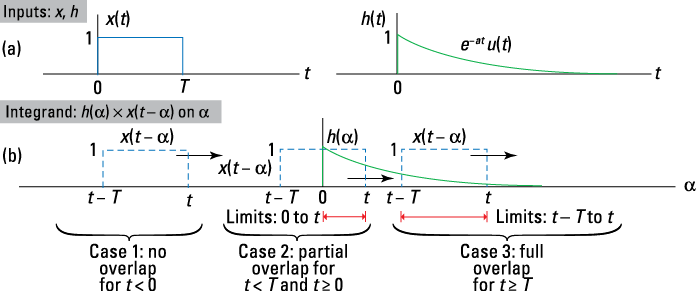
Figure 5-11: Convolution integral waveform sketches: the convolution inputs (a) and the integrand waveforms, , along the -axis (b), under Cases 1–3.

This problem breaks down into three cases.

• Case 1 is the no overlap condition, when . It follows that under this condition.

• Case 2 is partial overlap, which corresponds to . The active interval is thus .

• Case 3 is full overlap, which corresponds to .

3. Establish the integration limits from the waveform alignment.

From Figure 5-11, the integration limits under Cases 1 and 2 include the following:

• For Case 2, runs from 0 to t.

• For Case 3, runs from to t.

4. Integrate, and then move on.

• The Case 2 integration is .

• The Case 3 integration is .

Pulling all the pieces together into a case expression yields the following:

Figure 5-12 shows a family of output curves for and T varying from 1 to 10 s.

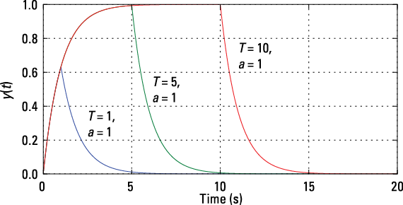
Figure 5-12: The result of convolving a pulse of duration T seconds with an exponential impulse response having time constant 1/a.

Example 5-4: Consider a 1-Hz sinusoid passing through a system having rectangular impulse response of amplitude 1/T and width T starting at t = 0. Start with the sinusoid turning on at by incorporating a unit step function; later, you can remove the step to see what it’s like to deal with an infinite duration signal.

The convolution setup is where . The output support interval is . Now you’re ready to work through the four steps:

1. Sketch the two waveforms of the integrand on the integration variable axis, in this case.

See the waveforms sketched in Figure 5-13a and the two waveforms of the integrand sketched on the in Figures 5-13b through 5-13d, as t takes on increasing values.

2. Find values of t (cases) where overlap (partial or full) occurs in the integrand.

This problem breaks down into three cases, shown in Figures 5-13b through 5-13d. These cases are identical to Example 5-3, except now you’re working on the -axis. See Figure 5-13 for details.

3. Establish the integration limits from the waveform alignment.

From Figure 5-13, the integration limits under Cases 2 and 3 (the overlap cases) also follow from Example 5-3, but now on the -axis.

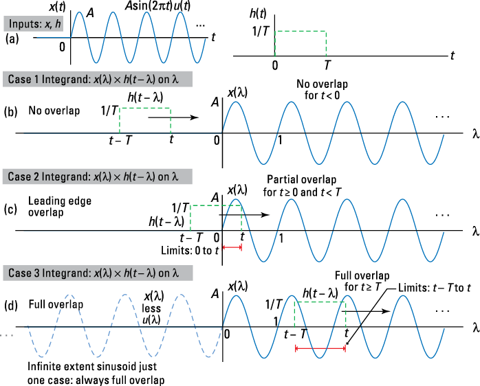
Figure 5-13: Convolution integral waveform sketches: the convolution inputs (a), integrand waveforms (b–d), under Cases 1–3, respectively.

4. Integrate, and then move on.

The Case 2 integration is

The Case 3 integration is

Note: From the geometric series sum formula (see Chapter 2), this expression can also be written as

The complete case expression is

If you remove from , the input sinusoid is now of infinite duration (see the dashing on the left side of Figure 5-13d), and you have only one case to consider. The output support interval is . The original Case 3 result provides the complete solution:

No matter what value you choose for t in , the signal is always nonzero on .

The semi-infinite and infinite input signal results are compared in Figure 5-14.

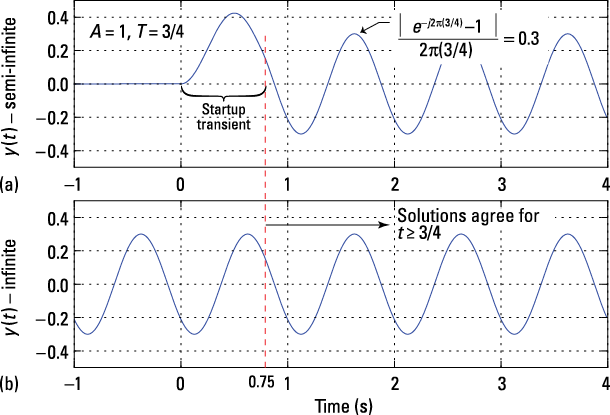
Figure 5-14: Semi-infinite and infinite input signal results of Example 5-4.

Stepping Out and More

The impulse response (IR) is closely related to the step response, which is another useful system characterization input signal. If you have the step response or the impulse response, you can find the other. Two for the price of one! You can establish this relationship through differentiation or integration, depending on the conversion direction.

The LTI specialization of this chapter also describes important stability and causality results. Stability and causality are directly related to the impulse response of a system, emphasizing the importance of a system’s IR.

Step response from impulse response

The impulse response completely characterizes an LTI system. To determine the output of a system with a unit step response as the input, you simply convolve the unit step signal (see Chapter 3) with the impulse response h(t). What more could you ask for?

The step response is defined as the system output, from an at-rest condition, when given a unit step input: . This is a popular characterizing waveform in control systems. Looks easy enough, right? Just another convolution. But wait! Maybe you want to investigate the details of the convolution integral.

Here, I expand the convolution integral for :

The final form follows by noting that turns off when , so I set the upper limit to t. The conclusion is that integrating the impulse response gives you the step response:

In the opposite direction, differentiating the step response returns you to the impulse response:

Did you really just read that? Yes! The step response is the integration of the impulse response, which is the derivative of the step response. This means that if you have h(t) or ys(t), you can compute the other.

BIBO stability implications

Bounded-input bounded-output (BIBO) stability (described in detail in Chapter 3) requires that the system output remains bounded for any bounded-input . When the system is also LTI, you can establish BIBO stability from the impulse response alone, by seeing whether .

Example 5-5: Consider . According to the LTI stability theorem, you need . Therefore, the system is BIBO stable. Note that the unit sets the integration lower limit to 0 in this ­calculation.

Causality and the impulse response

A system is causal if the present output relies only on past and present inputs. From an implementation perspective, causal means that the system can be implemented in real hardware. You want to be able to build what you design, right? In this section, I explore the connection between the system impulse response and causality, providing an easy way to spot causal systems.

For an LTI system, you have the convolution integral to establish the relationship between the input and output, along with the impulse response. How must be constrained to ensure causality? Consider the following:

From the last integral in the second line, you see that the system can’t use future inputs if for . Rewriting, a causal system has .

A direct consequence of the causality on is that the convolution limits are now constrained:

Example 5-6: Consider the moving-average system: .

You can find the impulse response for this system by setting :

Does the integration make sense? When you integrate the unit impulse, you get 1 as long as the impulse lies on the integration interval. The integration interval on the α is [–5, 5] in this case, which holds so long as . This describes a rectangle pulse centered at .

The present system is non-causal because for . The system averages inputs five seconds on either side of the present input to form the present output. You can make the system causal simply by shifting the impulse response five seconds to the right; for example, . Now you form the average by using inputs from zero to ten seconds in the past.