Chapter 6

Discrete-Time LTI Systems and the Convolution Sum

In This Chapter

Getting familiar with the impulse response and the convolution sum

Understanding the convolution sum and its properties

Figuring out convolution sum problems

Chances are good that sometime within the last 24 hours you’ve interfaced with an electronic device that uses a discrete-time linear time-invariant (LTI) system. In fact, you’ve probably done so with more than one device! Surprised? Maybe not. The candidate devices I have in mind are popular ones, including digital music players, cellphones, HDTVs, and laptop computers.

Another name for a discrete-time LTI system is digital filter, and I cover the analysis and design of digital filters over multiple chapters in this book. The emphasis in this chapter is the time-domain view. (Check out Chapter 11 for details on the frequency domain and Chapter 14 for information on the z-domain view.)

The drill down in this chapter on the time-domain analysis, design, and behavior of discrete-time LTI systems leads to discrete-time convolution, or the convolution sum. The convolution sum is the mathematics of processing the input signal to the output of a digital filter. A related time-domain topic, linear constant coefficient (LCC) difference equations, is covered in Chapter 7, where I explain that the LCC difference equation implementation of a discrete-time LTI system produces an efficient processing algorithm. (Say that three times fast.)

Specializing the Input/Output Relationship

A general system input/output relationship is described mathematically as y[n] = T{x[n]}, where T{} represents the system or operator of interest. Figure 6-1 shows this relationship in block diagram form. The operator T{} describes a mapping of the input sequence, x[n], to the output sequence, y[n].

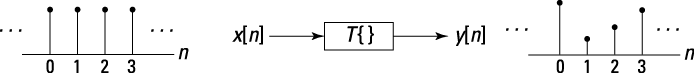
Figure 6-1: Block diagram depicting a general input/output relationship.

In Chapter 4, I define classifications of discrete-time systems. Here, I focus on systems that are both linear and time-invariant (LTI). I first describe the impulse response as a means to characterize an at-rest system (memory is set to zero). You can think of the impulse response as a form of system signature in the time domain. The fact that the system is time-invariant means that the impulse response is the same no matter when it’s applied to the system, less the time shift due to the application time. I then show that time invariance combined with system linearity makes it possible to express the system output as a linear combination of the input signal and the impulse response. This linear combination is given the special name convolution sum.

In real-world applications, most discrete-time systems are linear and time-invariant because the analysis and design of LTI systems are tractable and, in the vast majority of cases, bring satisfying results. After all, engineers are problem solvers with a finite number of tools who tend to pursue effective processes and reliable outcomes.

Using LTI systems and the impulse response (sequence)

The impulse response of a discrete-time LTI system, h[n], is defined as the output produced by an at-rest system, when given input . (Check out Figure 6-2 to see a graphical depiction of the input/output relationship.) The at-rest condition ensures that the resulting h[n] is due solely to the input sequence. Keep in mind that other characterizations are possible, too, such as the step response, which I describe in the section “Step response from the impulse response,” later in this chapter.

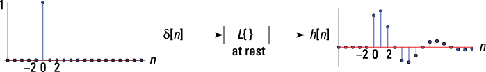
Figure 6-2: Depiction of the impulse response.

With information from the impulse response and the discrete-time LTI system input, you can calculate the output sequence via the convolution sum. The convolution sum for discrete-time systems is analogous to the convolution integral for continuous-time systems found in Chapter 5.

Getting to the convolution sum

To establish the convolution sum formula, any sequence x[n] can be expressed as a superposition of time-shifted impulse functions (flip to Chapter 4 for details):

Combining the preceding impulse function expansion with the LTI assumption leads to the following conclusion:

The * is the customary shorthand notation to convey convolution between x[n] and h[n]. This means — at last! — you’ve arrived at the famous convolution sum formula for computing the system output y[n] given the impulse response h[n] and input x[n]. Note that the two forms given are equivalent.

The doubly infinite sum is a necessary evil, because the support interval — the n-axis interval where x[n] and h[n] are nonzero — for both x[n] and h[n] could be .

---

---

The word convolve simply means “to roll or coil together; to entwine.” From the first form of the convolution sum, you combine/sum time-shifted copies of the impulse response h[n – k] weighted by the input sequence values x[k] that correspond to the time shift:

Example 6-1: To practice solving a convolution sum problem, consider a two-sample moving average system with a three-sample input sequence:

The is a timing mark used to denote where n = 0 in the sequences. This sequence notation is particularly convenient for finite duration sequences. Outside the interval shown, you can assume that the sequences are zero.

When the problem you’re working on is simple, you can get the answer quickly with a direct attack. In this case, take the second form of the convolution sum and insert h[n]:

The doubly infinite sum can be intimidating, but notice that h[0] = 1/2, h[1] = 1/2, and h[k] = 0 for all other values of k. Only two terms of the sum survive, so you can write

In words, the output is the average of the present input, x[n], and x[n – 1], which is the input itself, just one sample in the past. For the given input, this becomes

Check to see that the output is indeed a two-sample moving average of the input. The first output (at n = 0) is 1/2. The present input is 1, and the previous input is 0, making the average (0 + 1)/2 = 1/2. The second output (at n = 1) is 3/2. The average of the present and past inputs is (1 + 2)/2 = 3/2, the expected result. Note the present input, 2, averaged with the past input, 1, is indeed 3/2. You can check the last two nonzero outputs.

From this example, you can now state that for systems having finite impulse response (FIR), h[n] is of the form

It follows that .

The FIR nature of h[n] means that the limits in the convolution sum extend through [0, N], rather than . FIR systems, or filters, are common in today’s electronic applications. The action of the filter is to form the present output as a linear combination of N past inputs and the present input. Is this a causal (non-anticipatory) relationship? Yes, because future inputs aren’t used to form the present output.

Simplifying with Convolution Sum Properties and Techniques

To simplify convolution work and avoid careless errors, knowing some fundamental properties and techniques of working with the convolution sum is important. These properties and techniques are similar to those developed for the convolution integral (covered in Chapter 5), but for continuous-time systems, you deal with integrals instead of summations.

Applying commutative, associative, and distributive properties

Do the words commutative, associative, and distributive properties ring any bells? I don’t want to bring back terrifying memories from your past, but the convolution sum obeys these properties, which means you can write the properties given in Table 6-1.

Table 6-1 Convolution Sum Properties

Property	Formula
Commutative
Associative
Distributive

The block diagram relationships of Figure 6-3 show the commutative, associative, and distributive properties. Figure 6-3a describes the series (cascade) connection of two systems and follows from the associative property. The impulse response of the cascade is given by .

---

---

Figure 6-3b shows a parallel connection LTI system and follows from the second line of the distributive property. The impulse response of the parallel connection is given by .

Notice that these discrete-time cascade and parallel connections track the continuous-time case exactly (see Chapter 5). Here, the sequence notation indicates that you’re working with a discrete-time signal instead of a ­continuous-time signal.

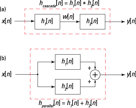
Figure 6-3: Block diagrams of a series or cascade connection (a) and a parallel connection (b) of LTI systems.

Convolving with the impulse function

In some situations, the convolution sum is just plain easy to work. One such situation is when you convolve anything (I mean any signal) with a time delayed (shifted) impulse function. You get that anything back, only time delayed by the delay factor of the impulse function.

Convolution with the impulse sequence, as in , is a freebie — meaning you have no real convolution to do; just evaluate the function at the location of the impulse it’s being convolved with and you’re done. Check it out (n0 is constant):

A simple extension result is .

Transforming a sequence

For discrete-time signals, you can perform time (sequence) shifting, axis flipping, and superimposing. These operations are useful for aligning multiple signals and for filtering applications, such as convolution. For details on these tasks as they apply to continuous-time signals, check out Chapter 3.

For example, the signal is shifted by samples. For , the shift is to the right, and for , the shift is to the left. The key observation is that by letting , you need to move forward in time by an additional steps to compensate for the in the argument of .

Both forms of the convolution sum formula require flipping and sliding (shifting) one of the two sequences. Sounds fun, right? This technique is vital to problem solving because no guessing is allowed; you have to pay attention to every detail to get the correct answer.

Flipping a signal is just changing the sign of the argument; that is, . The sequence value at is unchanged, but the values on the positive axis are now flipped to the negative axis, and those of the negative axis are flipped to the positive axis. In short, the flipping is with respect to . You can shift the flipping point to by writing .

With this information on shifting and flipping, consider the variable change , viewed on the k axis. A convenient way to view the shifted and flipped sequence is to write . Now with respect to the k axis, the sequence is flipped about the point . Changing n moves the flipped sequence along the k axis.

Example 6-2: Consider the sequence

Sketch , using Python. The custom function ex6_2(k) contained in ssd.py, generates x[k] given a time index array.

Then plot the two sequences, using a k-axis vector running over the interval [–10, 10]. Here’s an abbreviated version of the command line code. The plots are given in Figure 6-4.

In [800]: import ssd # needed for current session

In [801]: k = arange(-10,10) # k-axis for plotting

In [802]: stem(k,ssd.ex6_2(k)) # plot x[k]

In [804]: stem(k,ssd.ex6_2(-k),'g','go') # plot x[-k]

In [806]: stem(k,ssd.ex6_2(2-k),'r','ro') # plot x[2-k]

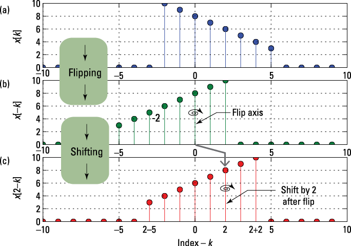
Figure 6-4: Stem plots of x[k] (a), x[–k] (flipped) (b), and x[2 – k] (shifted) (c) in which (c) is equivalent to a shift two units to the right and then a flip about that point.

To verify that all is well in the flip and shift, plug the edge k values into x[n – k] to see that the sequence support interval is consistent with the original x[n] sequence:

The left or trailing edge of is –2. With shifting and flipping, the index . The flipping action means that the left edge becomes the right edge of . For the case , the right edge is thus sitting at . Agreement with Figure 6-4c!

The right edge of is +5. With shifting and flipping, . Agreement with Figure 6-4c!

Solving convolution of finite ­duration sequences

As with the convolution integral of Chapter 5, you solve a convolution sum problem by starting from one of two forms of the sum argument: x[k]h[n – k] or x{n – k]h[k]. From there, you sum the product of the two sequences that form the sum argument.

As n increases from –∞ to ∞, h[n – k] slides from left to right along the k-axis. For each value of n, you consider the product x[k]h[n – k] and sum the nonzero or overlap intervals along the k-axis. For some problems, you have to consider a lot of different n values, but this is where using a table method is helpful. (I examine this method in the later section “Using spreadsheets and a tabular approach.” You can try your hand at the table method in Example 6-5.) For other problems, you find contiguous intervals of n values where you can use the geometric series sum formula (see Chapter 2). For the form h[k]x[n – k], do the same thing, except x[n – k] slides as n changes.

The general solution is piecewise, meaning expressions for y[n] are valid for some , which corresponds to case i, i = 1, . . . , N. When you put all the pieces together, you have a solution valid for .

Unlike the convolution integral, the convolution sum may have a support interval of a single point. The four steps in Figure 6-5, which parallel the ­continuous-time scenario of Chapter 5, outline the general solution procedure. Find a table-based method for solving this problem in Example 6-5.

Example 6-3: Consider the convolution of , using the convolution sum form .

Figure 6-6a shows the signal and impulse response to be convolved. Figure 6-6b shows both signals on the k-axis with n as a free variable. In Figures 6-6b through 6-6f, the flipped and shifted sequence h[n – k] is additionally positioned to various overlap cases. And Figure 6g shows the output.

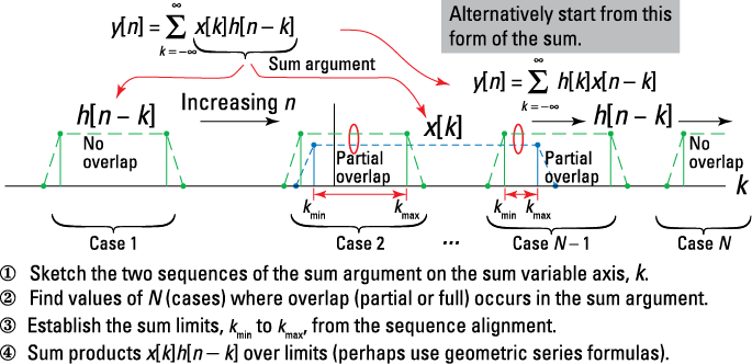
Figure 6-5: Four steps to solving a convolution sum problem and a graphical depiction of the cases as h[n – k] slides (shifts) from left to right.

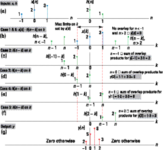
Figure 6-6: The convolution of x[n] with h[n]: the convolution inputs (a), the sum argument sequences x[k] and h[n – k] (b–f) under Cases 1–6, respectively, and the output y[n] (g).

Here are the steps you take to get y[n]:

1. Sketch the two sequences of the sum argument on the sum variable axis, k.

In Figure 6-6b, x[k] and h[n – k] are sketched for n < –1 and n > 2 along the k-axis. In Figures 6-6c through 6-6f, n is chosen to position h[n – k] at all the overlap cases of interest.

2. Find values of n (cases) where overlap occurs in the sum argument.

• Case 1 and Case 6 occur when n < –1 and n – 1 > 1 or n > 2, respectively. For Case 1, y[n] = 0 for n < –1, and for Case 6, y[n] = 0 for n > 2.

• Case 2 is what I call partial overlap leading edge. This occurs when n = –1.

• Case 3 is full overlap when n = 0.

• Case 4 is full overlap when n = 1.

• Case 5 is partial overlap trailing edge when n = 2.

3. Establish the sum limits from the sequence alignment.

With the help of Figure 6-6, the sum limits lie at most on the interval [–1, 1] but are less than this for the partial overlap cases.

• Under Case 2, the limit on k is simply k = –1.

• Under Case 3, the limits on k are –1 to 0.

• Under Case 4, the limits on k are 0 to 1.

• Under Case 5, the limit on k is simply 1.

4. Form the sum of products between the two sequences, and then move on.

• The Case 2 sum of overlap products is y[–1] = 2(1) = 2.

• The Case 3 sum of overlap products is y[0] = 1(1) + 2(2) = 5.

• The Case 4 sum of overlap products is y[–1] = 1(1) + 2(3) = 8.

• The Case 5 sum of overlap products is y[–1] = 1(3) = 3.

Example 6-4: In this example, I build on the pattern established by Example 6-2 to show you the support interval relationships for the convolution of two generic finite length sequences x[n] and h[n] (as shown in Figure 6-7).

In Figure 6-7, the support interval is displayed as a generic rectangle (dotted lines) for convenience. The reality is that any nonzero sequence value can appear on the closed intervals [n1, n2] and [n3, n4]. Here, x[n] has duration Nx and h[n] has duration Nh.

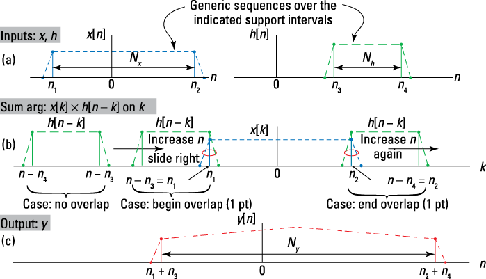
Figure 6-7: Convolving two generic finite length sequences: the convolution inputs (a), the sum argument sequences x[k] and h[n – k] along the k-axis (b), and the output y(t) (c).

In general you can call the duration of x[n] Nx and, similarly, for h[n], the duration is Nh. The subscript notation is commonly used in signals and systems; N is used for sequence duration (N = number of samples in a sequence, sequence length, and so forth). Adding the subscript clarifies that you’re talking about the duration of a specific sequence.

Now you can utilize your flipping and sliding skills to discover the support interval for y[n] in this general problem, where

You must evaluate the sum for each value of independent variable n. Nonzero results can occur only when the product x[k]h[n – k] ≠ 0 and terms don’t cancel. This analysis considers only the former situation, so the result is the largest possible support interval, barring any sum term cancellations to zero.

The following steps walk you through the process of determining the support interval of the convolution sum. Verifying the support interval before crunching the numbers of the convolution sum itself is important and helps you avoid having to do the whole thing over again. Note: The actual convolution sum isn’t computed in this example.

1. Sketch the two sequences of the sum argument on the sum variable axis, k.

Figure 6-7b shows a sketch of the two waveforms on the k-axis.

2. Find values of n (cases) where overlap occurs in the sum argument.

Refer to the example in Figure 6-7: As h[n – k] slides to the right for increasing n, overlap and the first nonzero value in the product occur when n – n3 = n1 or n = n1 + n3 — when the leading edge of h[n – k] just touches the trailing edge of x[k]. The last nonzero product occurs when the trailing edge of h[n – k] is just touching the leading edge of x[k]. Mathematically, the condition occurs when n – n4 = n2 or when n = n2 – n4.

3. Establish the sum limits from the sequence alignment.

The sum limits are set by the specific cases, so they don’t apply in this example. In a gross sense, all you can say is that the fixed sequence x[k] constrains the limits on k to be at most [n1, n2].

4. Form the sum of products between the two sequences, and then move on.

You don’t carry out the sum of products in this example.

This exercise reveals the following information about the properties or characteristics of the convolution of two finite duration sequences:

The nonzero output sequence y[n] begins at the sum of the x[n] and h[n] sequence starting points: n = n1 + n3.

The output sequence y[n] stops at the sum of the x[n] and h[n] sequence ending points: n = n2 + n4.

The output sequence y[n] has maximum support duration that’s equal to the sum of the durations of x[n] and h[n] minus 1: y[n] is nonzero on at most , so

As a bonus, the results for finite duration sequences easily extend to semi-infinite duration sequences (check out Examples 6-6 and 6-7).

If x[n] has support and h[n] has support [5, 20], then the output sequence y[n] support interval begins at 0 + 5 = 5 and ends at . The support interval for y[n] is and the duration is .

If x[n] and h[n] have support intervals and [0, 10] respectively, then the support interval for y[n] is . Know why? Minus infinity plus 0 is still minus infinity, and infinity plus 10 is still infinity.

In terms of actual convolution, there is always overlap between x[n] and some nonzero values of h[n].

Working with the Convolution Sum

In this section, I help you develop practical hands-on skills for solving convolution sum problems of all types. The first approach is table-based and intuitive. The second is more of a direct analysis attack, which works well when the sum expressions under various cases are actually summable in closed form, as when using geometric series sum formulas (see Chapter 2).

Using spreadsheets and a tabular approach

Example 6-5: A tabular approach works well for x[n] and h[n] finite duration sequences. Consider these sequences:

Decisions decisions . . . which form of the convolution sum should you use? The choice really comes down to comfort factor. You need to flip and slide one or the other sequence and do it without error. Choosing one over the other offers some flexibility. For me, I generally choose to flip and slide the least complex of the two sequences. You may see things differently and choose always to flip and slide the input x[n]. Here, I choose

Notice that the sum limits have already been constrained to the support interval for h[k]: .

Here’s a step-by-step solution and spreadsheet check:

1. Sketch the two sequences of the sum argument on the sum variable axis, k.

Get your bearings by making a quick sketch of h[k] stacked over x[n – k], such as the sketch in Figure 6-8.

2. Find values of n (cases) where overlap occurs in the sum argument.

Case 1 in Figure 6-8 occurs when n < –1; there’s no overlap. As x[n – k] slides to the right for increasing n, overlap (and the first nonzero value in the product) occurs when n = –1 — when the leading edge of x[n – k] just touches the trailing edge of h[k] at a single point. The last nonzero product occurs when n – 3 = 2 or n = 5 — when the trailing edge of h[n – k] is just touching the leading edge of x[k].

Cases 2 through 8 correspond to n stepping from –1 to 5. The table described later in Step 4 manages the seven overlap cases.

3. Establish the sum limits from the sequence alignment.

With the help of Figure 6-8, the sum limits are visible for each n (case) where overlap occurs. For example, n = 2 has full overlap, so you sum the h[k]x[n – k] products from k = –1 to k = 2. The table described in Step 4 can help you visualize the limits for all the overlap cases.

4. Form the sum of products between the two sequences, and then move on.

You set up a table (such as the one in Figure 6-9) to house the x[n – k] and h[k] values for each case, identify the sum limits, and perform the sum of products as n steps from –1 to 5 — truly the heart of the convolution sum. You use the sequence plots of h[n] and x[n – k] found in Figure 6-8 to make the table entries. You fill in entries for h[k] in the top center of the table and fill in x[n – k] in the rows below h[k] at the needed shift values for n. Using a spreadsheet table is optional; the table is more of a “housekeeping” means, so I recommend at minimum a blank table paper worksheet (great for your next quiz). The spreadsheet just automates the math, so it isn’t a requirement.

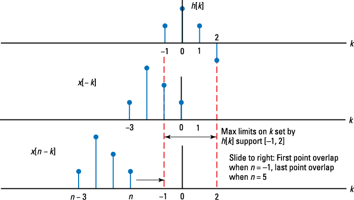
Figure 6-8: A sketch of h[k] and x[n – k] reveals that the sequence overlap begins at n = –1 and ends at n – 3 = 2 or n = 5.

Consider the case n = 2 as highlighted in Figure 6-9: .

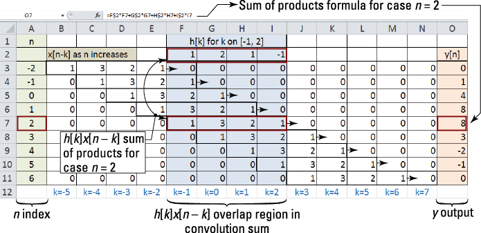
Figure 6-9: Convolution sum calculation for finite length sequences fit into a spreadsheet table.

As a check, see whether your results here agree with the bullet items found in Step 4 of Example 6-3. In particular, check that the first nonzero output is at the sum of the sequence starting points to find that n = –1 + 0 = –1. Now check that the last nonzero point is the sum of the sequence ending points to find that n = 2 + 3 = 5. The start and stop points agree with the table results.

5. As a final check, use IPython and the custom function conv_sum() to numerically convolve the two sequences and keep track of the time index n for plotting (find the function in the code module ssd.py).

The function makes use of the scipy subpackage signal for the underlying convolution function. The array x holds the x[n] values, and the array nx holds the corresponding time index. The array h holds the h[n] values, and the array nh holds the corresponding time index.

Here are the IPython commands to produce a numerical output:

In [418]: y,ny = ssd.conv_sum([1,2,3,1],[0,1,2,3],[1,2,1,-1],[-1,0,1,2]) # input x, nx, h, nh

In [419]: ny

Out[419]: array([-1, 0, 1, 2, 3, 4, 5]) # index values

In [420]: y

Out[420]: array([ 1, 4, 8, 8, 3, -2, -1])# Output y checks

Attacking the sum directly with geometric series

Purely analytical solutions provide valuable insights in the design of LTI systems. In the context of the convolution sum, consider the examples in this section. They’re all detailed in nature, and I use geometric series sum formulas to simplify solutions into a compact piecewise form. The goal in these examples, by the way, is to find .

Example 6-6: Consider a rectangular pulse sequence of duration N samples for both x[n] and h[n]: x[n] = h[n] = u[n] – u[n – N], using the convolution sum form .

To avoid careless errors in your preliminary analysis, check the support interval for the output, using the starting and ending point rules established in Example 6-3. The output starts at n = 0 + 0 = 0 and concludes at n = (N – 1) + (N – 1) = 2N – 2. These values guide the remaining steps.

Now follow the steps from Figure 6-5 to get y[n]:

1. Sketch the two sequences of the sum argument on the sum variable axis, k.

Figure 6-10a sketches x[k] and Figures 6-10b through 6-10e sketch h[n – k] for five different cases of overlap.

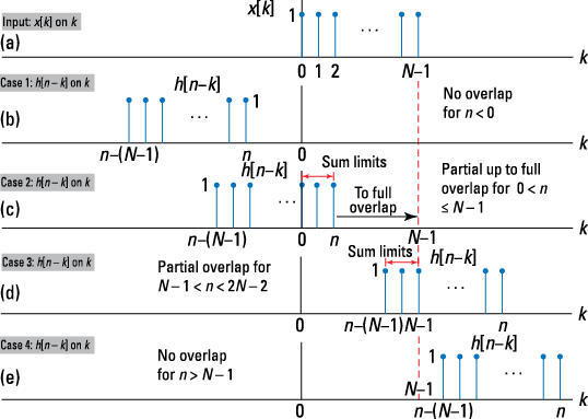
Figure 6-10: The convolution of x[n] with h[n]: the convolution input x[k] (a), the input h[n – k] (b–e) flipped and shifted to illustrate Cases 1–4.

2. Find values of n (cases) where overlap occurs in the sum argument.

• Case 1 and Case 4 occur when n < 0 and n – (N – 1) > N – 1 or n < 2N – 2, respectively. For Case 1, y[n] = 0 for n < 0; for Case 4, y[n] = 0 for n < 2N – 2.

• Case 2 is partial overlap of the leading edge leading to full overlap. This occurs when and n – (N – 1) < 0 or n < N – 1. An interval, as opposed to a single point, works here because the sequence product is simply .

• Case 3 is partial overlap of the trailing edge that occurs when or .

3. Establish the sum limits from the sequence alignment.

With the help of Figure 6-9, you can identify the sum limits.

• Under Case 2, the limits on k are 0 to n.

• Under Case 3, the limits on k are n – (N – 1) to N – 1.

4. Form the sum of products between the two sequences, and then move on.

The Case 2 sum of overlap products is

Note that when n = N – 1 (full overlap) the output achieves the maximum output value of N.

The Case 4 sum of overlap products is

Find the final answer by counting the number of ones being added together. The sum is the upper limit minus the lower limit plus one.

Finally, you can summarize (whew!) y[n] into a compact piecewise form:

In Chapter 5, an exercise in convolving two rectangle pulses (continuous-time) led to a triangle pulse. It may not be obvious from the piecewise form of y[n], but you should expect to have a similar result here. To see for yourself, plot y[n] by hand or use a tool. I use the Python function con_sum() to convolve two rectangle sequences, using the step function dstep() (you can find both functions in the code module ssd.py, which you must import into the IPython environment). The result is shown in Figure 6-11 and is triangular in shape, just as expected!

The IPython commands to produce the plot of Figure 6-11 are

In [187]: import ssd # to access module functions

In [188]: n = arange(-5,20) # time axis

In [189]: x = ssd.dstep(n) - ssd.dstep(n-10)# N=10 pulse

In [190]: y, ny = ssd.conv_sum(x, n, x, n) # x conv x

In [191]: stem(ny,y) # plot output

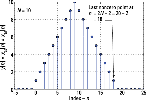
Figure 6-11: A plot of the convolution of two length ten rectangular pulse sequences using Python.

Example 6-7: Consider two semi-infinite duration sequences: a step function input x[n] = u[n] and an exponential impulse response h[n] = anu[n], where a is taken as a real constant with magnitude less than one.

I introduce these discrete-time signal types in Chapter 4 and explain that the function u[n] is the unit step function, which is 1 for and 0 for n < 0. From a systems-modeling standpoint, this example requires you to find the step response of the exponential decay system. (See the section “Connecting the step response and impulse response,” later in this chapter, to explore the relationship between the impulse response and the step response.)

On to the solution! Use direct substitution into the convolution sum formula:

This form of the convolution sum, I think, makes it easier to flip and shift u[n].

As preliminary analysis, the support interval for y[n] is .

With the preliminary analysis complete, you can jump right into the detailed step-by-step analysis:

1. Sketch the two sequences of the sum argument on the sum variable axis, k.

Figure 6-12a sketches h[k] and Figures 6-12b and 6-12c sketch x[n – k] for two different cases of overlap.

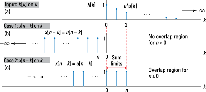
Figure 6-12: The convolution of x[n] with h[n]: the convolution input h[k] (a) and the input x[n – k] (b and c) flipped and shifted to illustrate Cases 1 and 2.

2. Find values of n (cases) where overlap occurs in the sum argument.

• Case 1 when n < 0 is no overlap so y[n] = 0.

• Case 2 occurs when .

3. Establish the sum limits from the sequence alignment.

With the help of Figure 6-12, you can identify the sum limits. Under Case 2, the limits on k are 0 to n.

4. Form the sum of products between the two sequences, and then move on.

Case 2 offers a bit of excitement — the limits and sum argument lead to a geometric series–based solution:

The summation form is picture perfect: a is the geometric series ratio. The series sums to 1 plus the ratio raised to one power higher than the upper sum limit all over the quantity 1 minus the ratio (find details on geometric series in Chapter 2).

Now you can combine the solution into a single expression by using the unit step function:

Figure 6-13 illustrates the general form of y[n]. The form of the step response is a charge-up that starts from 1 at n = 0 and reaches a steady-state value of 1/(1 – a). Why? For |a| < 1, large n has the quantity an + 1 → 0. This response is similar to the continuous-time step response of h(t) = e–atu(t) that I describe in Chapter 5.

Figure 6-13: The system response, y[n], for an input step (the step response).

Example 6-8: Consider an N-sample rectangular pulse input of the form x[n] = u[n] – u[n – N] and a system with exponential impulse response h[n] = anu[n]. This is a classic signal/impulse response pair-up.

You have options here! Brute-force plugging into the convolution sum works, but you can discover alternative methods from Example 6-7. As preliminary analysis, the support interval for y[n] is .

Here’s an alternative method, which utilizes basic convolution sum properties:

1. Use the distributive property of convolution to decompose y[n] into two terms by first substituting x[n] = u[n] – u[n – N]:

The third line follows from the distributive property, and the last term of the last line follows from time invariance.

2. Evaluate the convolution that remains (both terms of the last line).

This convolution is worked in Example 6-6, so now you just need to package up the pieces for this scenario:

You may be satisfied with the mathematical form you achieve in Step 2, but you get a different form of the same solution if you use the head-on convolution approach. It’s always good to see how additional manipulation can yield alternative (and sometimes more insightful) forms.

To find the alternative form, start by noting that for , only the first term is active; for , both terms are active, which means

In summary, the piecewise solution for y[n] is

The analysis reveals that as the rectangular pulse passes through the system, it goes through a charge-up phase (line 2) and then a discharge phase (line 3).

To see this graphically, write a Python function or simulate the output by using the convolution sum function used in Example 6-4 (be sure to import the ssd.py code module at command prompt when you start your IPython session). Using the simulation approach, first create the sequences x[n] and h[n]. The input, impulse response, and output sequences are created directly at the IPython command prompt. In the following example, I use subplots to stack all three sequences, but to save space, I don't show the plot labeling commands.

In [211]: import ssd # to access module functions

In [212]: nx = arange(0,10) # generate x[n]

In [213]: x = ssd.dstep(n) - ssd.dstep(n-5)

In [214]: nh = arange(0,15) # generate h[n]

In [215]: h = exp(-0.8*nh) # set a = 0.8

In [216]: y, ny = ssd.conv_sum(x,nx,h,nh) # convolve

See Figure 6-14 for a complete picture of all three sequences with the charge and discharge intervals evident.

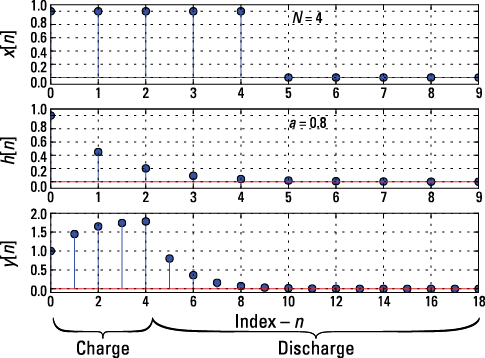
Figure 6-14: The input, impulse response, and output sequences for N = 4 and a = 0.8.

The action of the impulse response, which behaves as a low-pass filter when 0 < a < 1, is to slow down the edges of the rectangular pulse (refer to Figure 6-14). By slow down, I mean that when compared to the input x[n], which jumps up and down in one sample, the output y[n] slowly rises up starting at 0 and slowly falls back down starting at n = 4. Depending on the application, the filtering action in this example may be exactly what the design requires.

Think of the pulse signal as a simplified digital signaling waveform, such as an activation signal for opening a garage door. The system parameter a can be chosen to act as a sequence smoothing filter by choosing . Figure 6-14 illustrates this.

When you press the garage door button, it may bounce between zero and one before settling at one. With the filter, you need to hold the button down long enough (the pulse length N) for the filtered signal to rise above an amplitude threshold that toggles the door to either open or close. The filter reduces the chance of false triggering.

Example 6-9: Consider the cascade of two LTI systems, as shown in Figure 6-15.

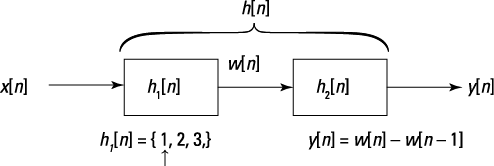
Figure 6-15: Finding the impulse response of a cascade of two LTI systems.

Next, I tell you how to find the impulse response of the cascade by using the table method, first shown in Example 6-5.

The impulse response you seek, h[n], is produced by (refer to Figure 6-3a).

How can you find h2[n]? Well, h2[n] is the impulse response of the second system. So if you force the input to the second system (called w[n] in Figure 6-15) to be , the output y[n] will be the impulse response, h2[n], by definition. Now, because you’re given , the resulting impulse response is . Now you have what you need to start crunching those numbers!

Note: This impulse response is an example of a simple difference equation (see Chapter 7 for the lowdown on simple difference equations).

The table in Figure 6-16 is set up to number crunch the answer, using the sum argument h1[k]h2[n – k]. From the support intervals of h1[n] and h2[n], the support interval for h[n] is [0 + 0, 2 + 1] = [0, 3]. As you work with the table, keep these limits in mind.

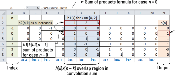
Figure 6-16: Spread­sheet table for convolving the impulse responses of the ­cascade.

Connecting the step response and impulse response

The step response is the output of an LTI system when driven by input x[n] = u[n]. To visualize that statement, consider the graphical depiction of Figure 6-17.

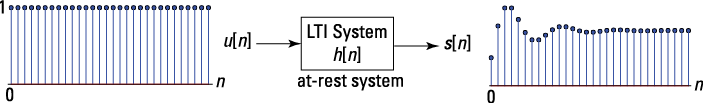
Figure 6-17: Graphical depiction of the step response.

The step response, denoted as s[n], is the system output for an at-rest system with input u[n]. You can establish the connection between the impulse response and step response rather easily. If you set n0 = 0 and x[n] = u[n] in the formula (introduced in the section “Convolving with the impulse function,” earlier in this chapter), it follows that .

This may seem like a lowly result, but if you consider u[n] (the unit step function) as the impulse response of an LTI system, the result is significant. Check out the upper path of Figure 6-18, where a cascade of a u[n] system with the h[n] system produces the step response when the cascade input is an impulse function.

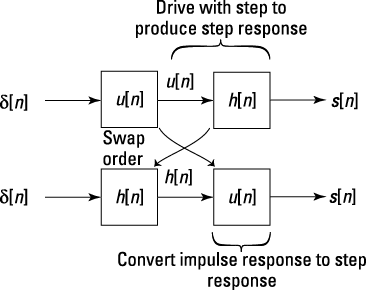
Figure 6-18: Block diagram explanation of the impulse response to step response transformation.

The u[n] system output is a step function. The commutative property of convolution says that the order of the cascade can be swapped, so you arrive at the second pathway in Figure 6-18, which shows s[n] is achieved from the impulse response by convolving h[n] with u[n].

Here’s how to connect the impulse response to the step response and the inverse:

1. Expand the convolution between the impulse response and the step response:

2. Set the upper sum limit to n by flipping and shifting the unit step, u[n – k].

3. Find the inverse relationship with a simple difference operation:

A system having u[n] as the impulse response is known as an accumulator. In transforming the impulse response to the step response, you witness the accumulator in action. The accumulator output is the accumulation, or sum, of all past inputs up to the present.

Example 6-7 revealed the step response of a system having exponential decay h[n] = anu[n] if |a|<1. With that information, you can find the step response through this relationship between the impulse and step responses:

It works! Flip back to Example 6-6 to see for yourself.

Checking the BIBO stability

Bounded-input bounded-output (BIBO) stability for discrete-time and continuous-time systems guarantees that the output remains bounded () for bounded () input. A system is BIBO stable if, for any bounded input, the output is also bounded.

When the system is LTI, BIBO stability follows if

The proof is straightforward:

Because if the input is bounded, the output is bounded if . This parallels the integral formulation for BIBO stability in Chapter 5.

Example 6-10: Consider the exponential impulse response h[n] = anu[n]. The LTI test for BIBO stability yields the following:

When a meets the following conditions, the sum is finite:

Case |a| < 1: From the infinite geometric series sum formula (covered in Chapter 2), you find that , so

.

Case : Under this condition, the sum diverges: .

Therefore, results in an unstable system.

This example also shows that a = 1, which implies h[n] = u[n] isn’t BIBO stable. But don’t let this worry you too much. Accumulators, which have h[n] = u[n], are still useful building blocks. The key is how they’re utilized in a composite system.

Checking for system causality

The key concept of causality for discrete-time systems is that present output values can rely on only past and present input values. Future input values have no influence on the present output. (Flip to Chapter 4 for more info on causality related to discrete-time systems.) For LTI systems, causality requires that the impulse response h[n] is 0 for n < 0. Figure 6-19 shows that only hb[n] is causal; both ha[n]and hc[n] are nonzero for n < 0.

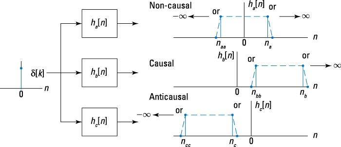
Figure 6-19: A depiction of causality for LTI systems in terms of the impulse response.

Example 6-11: Consider the following scenarios

Suppose that h1[n] = u[n + 5] – u[n – 10]. From the mathematical description, the impulse response turns on at n = –5 and turns off at n = 9. Five samples of the impulse response violate the LTI system causality requirement, so the system is non-causal.

Say that . The first term works because the step function doesn’t turn on until . The second term is an isolated sample sitting at n = –1, thus this system is non-causal.

Think about h3[n] = h2[n – 1]. If you move h2[n] one sample to the right, all is well — h3[n] = 0 for n < 0. This system is causal.

---

---